From nonlocal gap solitary waves to bound states in periodic media

Abstract

Solitary waves in one-dimensional periodic media are discussed employing the nonlinear Schrödinger equation with a spatially periodic potential as a model. This equation admits two families of gap solitons that bifurcate from the edges of Bloch bands in the linear wave spectrum. These fundamental solitons may be positioned only at specific locations relative to the potential; otherwise, they become nonlocal owing to the presence of growing tails of exponentially-small amplitude with respect to the wave peak amplitude. Here, by matching the tails of such nonlocal solitary waves, higher-order locally confined gap solitons, or bound states, are constructed. Details are worked out for bound states comprising two nonlocal solitary waves in the presence of a sinusoidal potential. A countable set of bound-state families, characterized by the separation distance of the two solitary waves, is found, and each family features three distinct solution branches that bifurcate near Bloch-band edges at small, but finite, amplitude. Power curves associated with these solution branches are computed asymptotically for large solitary-wave separation, and the theoretical predictions are consistent with numerical results.

1 Introduction

Nonlinear wave phenomena in periodic media are currently attracting a great deal of research interest in nonlinear optics, Bose–Einstein condensation and applied mathematics (see Christodoulides et al. 2003; Kivshar & Agrawal 2003; Morsch & Oberthaler 2006; Skorobogatiy & Yang 2009; Yang 2010 for reviews). Apart from scientific curiosity, this research activity is also driven by various potential applications, ranging from light routing in lattice networks (Christodoulides & Eugenieva 2001) to image transmission through nonlinear media (Yang et al. 2011).

A characteristic feature of periodic media is the existence of bands in the linear spectrum where linear disturbances, the so-called Bloch modes, may propagate. Between these Bloch bands are bandgaps in which linear disturbances are evanescent but nonlinear localized modes, commonly known as gap solitons, are possible. Since the first theoretical prediction (Christodoulides & Joseph 1988) and experimental observation (Eisenberg et al. 1998) of fundamental solitons in the semi-infinite bandgap of one-dimensional (1D) periodic waveguides, various types of gap solitons in one- and multi-dimensions have been reported theoretically and experimentally. Examples include 2D fundamental gap solitons, vortex solitons, dipole solitons, reduced-symmetry solitons, vortex-array solitons, truncated-Bloch-wave solitons and arbitrary-shape gap solitons (see Yang 2010 for a review). Multi-soliton bound states in periodic media have also been constructed in the framework of a discrete nonlinear Schrödinger (NLS) model (Kevrekidis et al. 2001). In addition, the stability of some of these gap solitons has been examined (Pelinovsky et al. 2004, 2005; Shi et al. 2008; Yang 2010; Hwang et al. 2011).

The plethora of gap solitons in periodic media calls for systematic identification and classification of the various types of solutions. On this issue, some progress has been made, particularly for gap solitons that bifurcate from linear Bloch modes at the edges of Bloch bands. Specifically, in 1D, only two gap-soliton families bifurcate from each edge of a Bloch band under self-focusing or self-defocusing nonlinearity (Neshev et al. 2003; Pelinovsky et al. 2004; Hwang et al. 2011), and the positions of these solitons relative to the periodic medium (or potential) are determined by a certain recurrence relation (Hwang et al. 2011). In 2D, four gap-soliton families (or a multiple of four families) bifurcate from each edge of a Bloch band under self-focusing or self-defocusing nonlinearity (Yang 2010).

However, for the majority of gap solitons, that do not bifurcate from band edges, systematic theoretical treatment is lacking at present. Numerical results indicate that, typically, those solution families feature multiple branches which bifurcate near band edges at small (but finite) amplitude (see Yang 2010 and references therein), yet there has been no analytical explanation for this phenomenon.

In this article, we employ the NLS equation with a spatially periodic potential to analytically construct and classify a broad class of gap solitons that bifurcate away from band edges in 1D periodic media. Our approach is based on the observation that the two families of fundamental gap solitons that bifurcate from a band edge can be located only at specific positions relative to the underlying potential; otherwise, they would be nonlocal owing to the presence of growing tails of exponentially-small amplitude with respect to the peak wave amplitude. However, by piecing together such nonlocal solitary waves, it is possible to construct higher-order gap solitons, or bound states. The proposed asymptotic theory is illustrated by working out details for bound states involving two nonlocal solitary waves. We show that a countable set of bound-state families can be constructed. Each family is characterized by the separation distance of the two solitary waves involved, and features three distinct solution branches that bifurcate near band edges. The analytical predictions are verified by comparison with numerical results.

2 Preliminaries

Our study of nonlinear wave phenomena in periodic media is based on the 1D NLS equation,

$$i\Psi_{t}+\Psi_{xx}-V(x)\Psi+\sigma\Psi^{2}\Psi^{*}=0$$ (1)

with a periodic potential $V(x)$ and self-focusing ($\sigma=1$) or self-defocusing ($\sigma=-1$) cubic nonlinearity. This equation is the appropriate mathematical model for Bose–Einstein condensates loaded in optical lattices (Dalfovo et al. 1999; Morsch & Oberthaler 2006) and laser beam transmission in photonic lattices under the paraxial approximation (Yang 2010). Although it is possible to consider a general periodic potential $V(x)$ as in Hwang et al. (2011), here, for simplicity, we shall work with the sinusoidal potential

$$V(x)=V_{0}\sin^{2}x\,,$$ (2)

which is $\pi$-periodic and also symmetric in $x$, $V_{0}$ being the potential depth. This potential frequently arises in nonlinear optics and Bose–Einstein condensates.

Solitary-wave solutions of (1) are sought in the form

$$\Psi(x,t)=\psi(x){\rm e}^{-i\mu t}\,,$$ (3)

where $\mu$ is the propagation constant, and the amplitude function $\psi(x)$ is real-valued and localized in space. Inserting (3) into (1), we find that $\psi(x)$ satisfies

$$\psi_{xx}-V(x)\psi+\mu\psi+\sigma\psi^{3}=0\,.$$ (4)

For infinitesimal solutions $\psi(x)$, the nonlinear term in the above equation drops out. The resulting linear version of (4) is a Mathieu-type equation and, by the Bloch–Floquet theory, its wave spectrum features a band–gap structure. Specifically, the linear version of (4) admits two linearly independent solutions in the form

$$p(x;\mu)={\rm e}^{ikx}\tilde{p}(x;\mu)\,,$$ (5)

with $\tilde{p}(x;\mu)$ being $\pi$-periodic in $x$. The wave character of these so-called Bloch modes hinges on whether the corresponding wavenumber $k$ is real or complex. By requiring $k$ to be real, one then obtains an infinite number of Bloch bands for $\mu$ in which the Bloch modes (5) propagate. These propagation bands are separated by gaps, where $k$ turns out to be complex, implying evanescent behaviour.

At the edges of Bloch bands, where the modes (5) switch from propagating to evanescent, two Bloch modes in the band collide at either $k=0$ or $k=\pm 1$, and a single real-valued Bloch mode that is either $\pi$- or $2\pi$-periodic, arises there. This suggests that edges of Bloch bands are possible bifurcation points of solitary-wave solutions of the nonlinear equation (4). These solitary waves reside inside band gaps and are the so-called gap solitary waves (or gap solitons).

The bifurcation of 1D gap solitons from band edges was discussed by Pelinovsky et al. (2004) using a multiple-scale expansion in powers of the wave amplitude, along with a certain constraint obeyed by locally confined solutions of (4). They identified two families of gap solitons that bifurcate from each band edge, namely ‘on-site’ and ‘off-site’ solitons, depending on whether the soliton is centred at a minimum or maximum of the sinusoidal potential (2).

More recently, Hwang et al. (2011) re-visited the problem of small-amplitude gap solitons near band edges, taking a different approach, that is applicable for a general potential $V(x)$. Rather than the constraint utilized in Pelinovsky et al. (2004), Hwang et al. (2011) focused on the behaviour of the tails of Bloch-wave packets. These tails are controlled by the coupling of the wave envelope to the periodic Bloch mode at the band edge, an effect that lies beyond all orders of the usual multiple-scale expansion in powers of the wave amplitude. Hwang et al. (2011) carried this expansion beyond all orders using techniques of exponential asymptotics (Yang & Akylas 1997), for the case of Bloch-wave packets whose envelope features a single hump. It turns out that the tails of such wave packets decay as $x\to\pm\infty$, and hence gap solitons arise, only for two specific locations of the wave envelope relative to the underlying periodic potential. Both these soliton families bifurcate from the linear (infinitesimal) periodic Bloch mode at a band edge, and they coincide with the on-site and off-site gap solitons found by Pelinovsky et al. (2004) in the case of a symmetric periodic potential.

In the present work, making use of the asymptotic expressions derived in Hwang et al. (2011) for the tails of a single-hump Block-wave packet, we shall construct small-amplitude gap-soliton families, in the form of bound states, that comprise two or more such wave packets. In contrast to the so-called fundamental gap solitons found in Pelinovsky et al. (2004) and Hwang et al. (2011), these higher-order soliton families bifurcate at small but finite amplitude close to a band edge, and they feature multiple branches that do not connect to fundamental soliton families or band edges.

In preparation for the ensuing analysis, we now summarize the main results of the multiple-scale perturbation procedure for a single-hump Bloch-wave packet (Pelinovsky et al. 2004; Hwang et al. 2011). Close to a band edge $\mu=\mu_{0}$, say, gap solitons are expected to be weakly nonlinear Bloch-wave packets. The solution to equation (4) is expanded in powers of an amplitude parameter, $0<\epsilon\ll 1$,

$$\psi=\epsilon\psi_{0}+\epsilon^{2}\psi_{1}+\epsilon^{3}\psi_{2}+\cdots,$$ (6)

along with

$$\mu=\mu_{0}+\eta\epsilon^{2},$$ (7)

where $\eta=\pm 1$,

$$\psi_{0}=A(X)p(x),$$ (8)

$p(x)\equiv p(x;\mu_{0})$, and $X=\epsilon x$ is the ‘slow’ variable of the envelope function $A(X)$. By imposing the appropriate solvability condition at $O(\epsilon^{3})$, it turns out that $A(X)$ satisfies the stationary NLS equation

$$DA_{XX}+\eta A+\sigma\alpha A^{3}=0\,,$$ (9)

where

$$D=\textstyle\frac{1}{2}\hskip 1.70709pt{\rm d}^{2}\mu/{\rm d}k^{2}\,|_{\mu=\mu_{0}}\,,\qquad\alpha={\int_{0}^{2\pi}p^{4}(x)\,{\rm d}x\bigg{/}\int_{0}^{2\pi}p^{2}(x)\,{\rm d}x}\,.$$ (10)

The well-known soliton solution of (9) is

$$A(X)=a\mathop{\rm sech}\nolimits{X-X_{0}\over\beta}\,,$$ (11)

where

$$a=\sqrt{2/\alpha}\,,\qquad\beta=\sqrt{|D|}\,,$$ (12)

and $X_{0}=\epsilon x_{0}$ denotes the position of the peak of the envelope. This solution exists provided $D\eta<0$ and $D\sigma>0$; the first of these conditions requires $\mu$ to lie in the interior of the band gap, while the second condition can be met in the presence of self-focusing ($\sigma=1$) nonlinearity if $D>0$, or self-defocusing ($\sigma=-1$) nonlinearity if $D<0$.

It is important to note that the envelope equation (9) is translation-invariant, and $X_{0}$ is a free parameter in the solution (11). As a result, gap solitons of equation (4) could be obtained regardless of the position of the envelope (11) relative to the underlying periodic potential. This conclusion would seem rather suspicious, though, given that the original amplitude equation (4) is not translation-invariant.

This issue was recognized by Pelinovsky et al. (2004), who pointed out that locally confined solutions of (4) must obey the constraint

$$M(x_{0})=\int_{-\infty}^{\infty}V^{\prime}(x)\psi^{2}(x;x_{0}){\rm d}x=0\,,$$ (13)

which can be readily obtained by multiplying (4) with $\psi_{x}$ and integrating with respect to $x$. Upon inserting the perturbation solution (6) and the potential (2) into (13), this condition then restricts the peak of the envelope to be at either a minimum ($x_{0}=0$) or a maximum ($x_{0}=\pi/2$) of the potential (2), corresponding to on-site or off-site gap solitons, respectively. It is also worth noting that the so-called Melnikov function $M(x_{0})$ in (13), which depends on the shift $x_{0}$ of the envelope relative to the potential $V(x)$, is exponentially small with respect to $\epsilon$; hence, the constraint (13) for possible locations of gap solitons hinges upon information beyond all orders of the two-scale expansion (6).

3 Nonlocal solitary waves

Another way of reconciling the two-scale expansion (6) with the fact that gap solitons can be placed only at specific locations relative to the potential $V(x)$, is by examining the behaviour of the tails of Bloch-wave packets near a band edge. Assuming that they have infinitesimal amplitude, these tails are governed by the linear version of equation (4). Hence, for $\mu$ inside a band gap and close to the edge $\mu_{0}$, using the same notation as in (7) and (10), the asymptotic representation of $\psi(x)$ away from the solitary-wave core is, generically, a linear combination of two evanescent Bloch modes

$$\psi_{\pm}(x)=p(x)\exp\bigg{\{}\pm\bigg{(}{\mu_{0}-\mu\over D}\bigg{)}^{\frac{1}{2}}x\bigg{\}}\,,$$ (14)

to leading order in $|\mu-\mu_{0}|=\epsilon^{2}\ll 1$. As expected, the slow exponential growth/decay of these modes is consistent with the behaviour of the tails of the envelope function $A(X)$ according to the steady NLS equation (9).

Now, for the purpose of constructing a solitary-wave solution of (4), the left-hand tail must involve only $\psi_{+}(x)$, $\psi(x)\sim\epsilon\hskip 1.13791ptC_{+}\psi_{+}(x)$, so that $\psi\to 0$ as $x\to-\infty$. For generic values of $C_{+}$, when one integrates equation (4) from this left-hand tail to the right-hand side, the right-hand tail would involve both $\psi_{-}(x)$ and $\psi_{+}(x)$,

$$\psi(x)\sim\epsilon\,C_{-}\psi_{-}(x)+E_{+}\psi_{+}(x)\qquad(x\gg 1)\,,$$ (15)

so $\psi(x)$ is not locally confined. However, the amplitude $E_{+}$ of the growing tail in (15) is exponentially small with respect to $\epsilon$ (see below), and hence this tail cannot be captured by an expansion in powers of $\epsilon$, such as (6). Only when $C_{+}$ takes certain special values can the growing-tail amplitude $E_{+}$ vanish, resulting in a true solitary wave solution. This restriction on $C_{+}$ is consistent with the integral constraint (13) utilized by Pelinovsky et al. (2004).

Hwang et al. (2011) computed the amplitude $E_{+}$ by carrying expansion (6) beyond all orders of $\epsilon$ for a general periodic potential $V(x)$, utilizing an exponential-asymptotics procedure in the wavenumber domain (Akylas & Yang 1995; Yang & Akylas 1997). According to this revised perturbation analysis, $E_{+}$, which indeed is exponentially small with respect to $\epsilon$, does vanish for two specific positions of the envelope (11) relative to the underlying potential, thus furnishing two families of gap solitons that bifurcate at the band edge. For the symmetric periodic potential (2), in particular, $E_{+}$ vanishes when the peak of the envelope is placed at $x_{0}=0$ or $x_{0}=\pi/2$, corresponding to the on-site and off-site gap solitons, as was obtained earlier by Pelinovsky et al. (2004).

As the details of the exponential-asymptotics procedure are rather involved, we shall only quote the main results. When the peak of the envelope (11) is not at a minimum or maximum of the potential ($x_{0}\neq 0,\pi/2$), the resulting ‘solitary’ waves are nonlocal owing to the presence of both growing and decaying solutions (14) in at least one of the tails. Specifically, assuming that the left-hand tail is locally confined in accordance with (6) and (11),

$$\psi\sim 2\epsilon\hskip 0.56917ptap(x){\rm e}^{\epsilon(x-x_{0})/\beta}\qquad(x\to-\infty)\,,$$ (16a)

the right-hand tail features a growing component of exponentially-small amplitude with respect to $$\epsilon$$, in addition to a decaying component analogous to (16a):

$$\psi\sim \ 2\epsilon\hskip 0.56917ptap(x){\rm e}^{-\epsilon(x-x_{0})/\beta}$$

$$+4\pi C{\beta^{3}\over\epsilon^{3}}{\rm e}^{-\pi\beta/\epsilon}\sin 2x_{0}\,p(x){\rm e}^{\epsilon(x-x_{0})/\beta}\qquad(x-x_{0}\gg 1/\epsilon)\,.$$ (16b)

Note that the amplitude of the growing tail in (16b) is proportional to a constant $C$. As explained in Hwang et al. (2011), this constant is determined from solving a certain recurrence relation that contains information beyond all orders of expansion (6). In particular, $C>0$ for the sinusoidal potential (2). As expected, the growing component of the right-hand tail (16b) is absent when $x_{0}=0,\pi/2$.

By utilizing the symmetries of equation (4) as noted below, it is straightforward to deduce from (16) the asymptotic behaviour of nonlocal solitary waves whose right-hand tail is locally confined,

$$\psi\sim 2\epsilon ap(x){\rm e}^{-\epsilon(x-x_{0})/\beta}\qquad(x\to+\infty)\,,$$ (17a)

but the left-hand tail comprises a growing and a decaying component:

$$\psi\sim \ 2\epsilon ap(x){\rm e}^{\epsilon(x-x_{0})/\beta}$$

$$-4\pi C{\beta^{3}\over\epsilon^{3}}{\rm e}^{-\pi\beta/\epsilon}\sin 2x_{0}\,p(x){\rm e}^{-\epsilon(x-x_{0})/\beta}\qquad(x-x_{0}\ll-1/\epsilon)\,.$$ (17b)

For the symmetric potential (2), equation (4) is invariant with respect to reflection in $x$ $(x\rightarrow-x)$, and the Bloch wave $p(x)$ at a band edge is either symmetric or antisymmetric in $x$, $p(-x)=\pm p(x)$. Since (4) is also invariant with respect to $\psi\to-\psi$, the reflected solution $\psi$ may thus be written as (17) for both symmetric and antisymmetric $p(x)$. The asymptotic expressions (16) and (17) for the tails of nonlocal solitary waves are key to constructing new families of locally confined solutions, in the form of bound states, as discussed below.

4 Bound states

As indicated above, gap solitons in the form of Bloch-wave packets with the ‘sech’ envelope (11) arise only when the peak of the envelope is at a minimum ($x_{0}=0$) or a maximum ($x_{0}=\pi/2$) of the potential (2). Apart from these fundamental soliton states, it is possible, however, to construct other gap-soliton families by piecing together two or more of the nonlocal solitary waves found in §3. The overall strategy for determining these so-called bound states is similar to that followed in Yang & Akylas (1997) for constructing multi-packet solitary-wave solutions of the fifth-order KdV equation. Here, we shall work out the details of finding bound states involving two Bloch-wave packets.

4.1 Matching of tails

Consider two nonlocal solitary-wave solutions, $\psi^{+}(x)$ and $\psi^{-}(x)$, whose ‘sech’-profile envelope functions are centred at $x_{0}^{+}$ and $-x_{0}^{-}$, respectively, with $x_{0}^{\pm}>0$. In addition, let $\psi^{\pm}(x)\to 0$ as $x\to\pm\infty$, so the right-hand tail of $\psi^{-}(x)$ and the left-hand tail of $\psi^{+}(x)$ are nonlocal. Let us define the separation between the solitary-wave cores of the two constituent nonlocal waves as

$$S\equiv x_{0}^{+}+x_{0}^{-}.$$ (18)

Then, assuming $S\gg 1/\epsilon$, (16b) and (17b) are legitimate asymptotic expressions for these tails in the ‘overlap’ region $-x_{0}^{-}\ll x\ll x_{0}^{+}$. Specifically, according to (16b), the right-hand tail of $\psi^{-}(x)$ is given by

$$\psi^{-}\sim\pm 2\epsilon a\hskip 1.42271pt{\rm e}^{-\epsilon(x+x_{0}^{-})/\beta}p(x)\mp 4\pi C{\beta^{3}\over\epsilon^{3}}{\rm e}^{-\pi\beta/\epsilon}\sin 2x_{0}^{-}\,{\rm e}^{\epsilon(x+x_{0}^{-})/\beta}p(x)\,,$$ (19)

and, according to (17b), the left-hand tail of $\psi^{+}(x)$ reads

$$\psi^{+}\sim 2\epsilon a\hskip 1.42271pt{\rm e}^{\epsilon(x-x_{0}^{+})/\beta}p(x)-4\pi C{\beta^{3}\over\epsilon^{3}}{\rm e}^{-\pi\beta/\epsilon}\sin 2x_{0}^{+}\,{\rm e}^{-\epsilon(x-x_{0}^{+})/\beta}p(x)\,.$$ (20)

Note that the upper sign in (19) corresponds to the case where the envelopes of the two solitary waves have the same polarity (sign), while the lower sign pertains to the case of opposite polarity.

Now, in order for these two nonlocal solitary waves to form a bound state, their growing and decaying tail components must match smoothly in the overlap region between the two main cores. Based on (19) and (20), this requires

$$\sin 2x_{0}^{-}=\sin 2x_{0}^{+}=\mp{a\over 2\pi C}{\epsilon^{4}\over\beta^{3}}{\rm e}^{\pi\beta/\epsilon}\,{\rm e}^{-\epsilon S/\beta}\,,$$ (21)

and, for this matching condition to be met, it is necessary that

$${a\over 2\pi C}{\epsilon^{4}\over\beta^{3}}{\rm e}^{\pi\beta/\epsilon}\,{\rm e}^{-\epsilon S/\beta}\leq 1\,.$$ (22)

Clearly, owing to the growing exponential ${\rm e}^{\pi\beta/\epsilon}$ on the left-hand side of (22), this constraint cannot be satisfied for $\epsilon\to 0$ when $S$ is finite. As a result, solution families of bound states are expected to bifurcate at a finite amplitude $\epsilon=\epsilon_{c}$, say, depending on the separation distance $S$. Below, we shall verify this claim and compute $\epsilon_{c}$ for the various solution branches.

4.2 Solution branches

Attention is now focused on the matching condition (21), in order to delineate the solution branches of bound states that bifurcate close to a band edge.

Consider first the case where the two nonlocal solitary waves have envelopes with the same polarity. Then, the upper sign applies in (21), and $\sin 2x_{0}^{-}=\sin 2x_{0}^{+}<0$. This condition can be satisfied in two ways:

$${\rm(i)}\quad x_{0}^{-}=(m+{\textstyle\frac{1}{2}})\pi+d\,,\qquad x_{0}^{+}=(n-{\textstyle\frac{1}{2})}\pi+d\,;$$ (23a)

$${\rm(ii)}\quad x_{0}^{-}=(m+{\textstyle\frac{1}{2}})\pi+d\,,\qquad x_{0}^{+}=n\pi-d\,,$$ (23b)

where $m$, $n$ are integers and $0<d<\pi/2$. Accordingly, the solitary-wave separation (18) corresponding to these two possibilities is

$${\rm(i)}\quad S=N\pi+2d\,;\qquad{\rm(ii)}\quad S=(N+{\textstyle\frac{1}{2}})\pi\,,$$ (24)

where $N=m+n$. Moreover, the matching condition (21) reads

$$\sin 2d={a\over 2\pi C}{\epsilon^{4}\over\beta^{3}}{\rm e}^{\pi\beta/\epsilon}\,{\rm e}^{-\epsilon S/\beta}\,,$$ (25)

with $S$ given by (i) and (ii) in (24).

It is convenient to label families of bound states by the integer $N$ which, in view of (24), controls the separation between the two nonlocal solitary waves that form the bound states. As noted earlier, the present theory assumes that these solitary waves are well-separated, namely, $S\gg 1/\epsilon$, which in turn requires $N\gg 1/\epsilon$; the validity of this condition will be verified later in this section.

In preparation for tracing the solution branches of the family of bound states corresponding to a given $N$, we write

$$d=\pi/4+\delta,$$ (26)

with $-\pi/4<\delta<\pi/4$, so that from (24), we have

$${\rm(i)}\quad S=S_{0}+2\delta\,;\qquad{\rm(ii)}\quad S=S_{0}\,,$$ (27)

where $S_{0}=(N+\frac{1}{2})\pi$. The matching condition (25), with $S$ given by (i) and (ii) above, then leads to the following two conditions, respectively,

$$\cos 2\delta=W(\epsilon,N)\,{\rm e}^{-2\epsilon\delta/\beta}\,,$$ (28a)

$$\cos 2\delta=W(\epsilon,N)\,,$$ (28b)

where

$$W(\epsilon,N)={a\over 2\pi C}{\epsilon^{4}\over\beta^{3}}{\rm e}^{\pi\beta/\epsilon}{\rm e}^{-\epsilon S_{0}/\beta}\,.$$ (29)

Based on equations (28), given $\epsilon$, one may find the values of $\delta$, and from (27) the corresponding separations $S$, for which bound states are possible.

Specifically, from equation (28a), it is easy to see that two values of $\delta$ arise for each $\epsilon$ above a certain threshold, $\epsilon_{c}^{(1)}$, which is the bifurcation point of the bound states obeying (28a). This threshold is associated with a double root, $\delta=\delta_{c}^{(1)}$, of equation (28a), where

$$\left.{\partial\over\partial\delta}\left(\cos 2\delta-W(\epsilon_{c}^{(1)},N)\,{\rm e}^{-2\epsilon_{c}^{(1)}\delta/\beta}\right)\right|_{\delta=\delta_{c}^{(1)}}=0\,.$$ (30)

From this equation and (28a), it follows that

$$\delta_{c}^{(1)}=\frac{1}{2}\tan^{-1}{\epsilon_{c}^{(1)}/\beta}.$$ (31)

Inserting this result into (28a), $\epsilon_{c}^{(1)}$ then is found by solving

$$\cos\big{(}\tan^{-1}{\epsilon_{c}^{(1)}\over\beta}\big{)}=W(\epsilon_{c}^{(1)},N)\exp\bigg{\{}-{\epsilon_{c}^{(1)}\over\beta}\tan^{-1}{\epsilon_{c}^{(1)}\over\beta}\bigg{\}}\,.$$ (32)

For $N\gg 1$, the two solution branches of $\delta(\epsilon)$, obtained from (28a) for $\epsilon>\epsilon_{c}^{(1)}$, are plotted schematically in figure 1. The bifurcation point $\epsilon_{c}^{(1)}$ is the turning point of this double-branch curve, and $\delta_{c}^{(1)}>0$. For $\epsilon\gg\epsilon_{c}^{(1)}$, it is clear from (28a) that $\cos 2\delta\to 0$, and hence the two branches approach $\delta=\pm\pi/4$, so $d=\pi/4+\delta\to\pi/2,0$. Therefore, in this limit, in view of (23a), the two solution branches that bifurcate at $\epsilon_{c}^{(1)}$ approach limiting configurations of bound states, with both solitary waves being on-site on one branch (as $\delta\to\pi/4$) and off-site on the other branch (as $\delta\to-\pi/4$). In other words, as the solution curve in figure 1 is traced from one branch to the other, the two solitary waves making up the bound state transform simultaneously from on-site to off-site. In this transition, $\delta$ decreases from $\pi/4$ to $-\pi/4$, and according to (i) in (27), the separation distance $S$ of the two solitary waves decreases from $(N+1)\pi$ to $N\pi$. This transition behaviour will be verified numerically in §6; see figure 2.

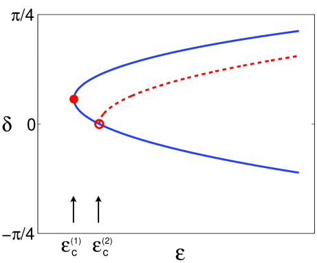
Figure 1: Schematic diagram for the three branches of the solution curve $\delta(\epsilon)$. Two branches (solid blue) are obtained from solving (28a) and one branch (dashed red) from solving (28b). The bifurcation point $\epsilon_{c}^{(1)}$ with $\delta_{c}^{(1)}>0$ (solid dot) is found by solving (32), and the bifurcation point $\epsilon_{c}^{(2)}$ with $\delta_{c}^{(2)}=0$ (open dot) is found by solving (34). (Online version in colour.)

Turning next to the second possibility of bound states in (27), equation (28b) furnishes two values of $\delta$,

$$\delta=\pm\frac{1}{2}\cos^{-1}W(\epsilon,N),$$ (33)

for each $\epsilon$, as long as $W(\epsilon,N)\leq 1$. Hence, $\epsilon$ must exceed a certain threshold, $\epsilon\geq\epsilon_{c}^{(2)}$, where $W(\epsilon_{c}^{(2)},N)=1$. In view of (29), this bifurcation point is determined from the equation

$${\pi\beta\over\epsilon_{c}^{(2)}}-{\epsilon_{c}^{(2)}S_{0}\over\beta}=\ln\bigg{[}{2\pi C\over a}\cdot{\beta^{3}\over\epsilon_{c}^{(2)^{4}}}\bigg{]}\,.$$ (34)

Here, the two values of $\delta$ in (33) actually correspond to equivalent bound-state configurations (under mirror reflection of the $x$-axis), as can be easily verified from (23b) with $d=\frac{1}{4}\pi+\delta$. Therefore, (28b) describes only one solution branch. For $\epsilon\gg\epsilon_{c}^{(2)}$, in particular, $\delta\to\pm\pi/4$, and this solution branch approaches a limiting bound-state configuration that, according to (23b), involves an on-site and an off-site solitary wave.

We remark that the double root $\delta=\delta_{c}^{(2)}=0$ of (28b) for $\epsilon=\epsilon_{c}^{(2)}$ is also a solution of (28a) for the same value of $\epsilon$. Hence, the solution branch (28b) bifurcates from the point $\delta=0$ on the lower branch of the solutions (28a), which themselves bifurcate at $\epsilon_{c}^{(1)}$, as illustrated schematically in figure 1. As a consequence, the bound-state family corresponding to a certain $N$ comprises three distinct solution branches which are connected with each other. The bifurcation points, $\epsilon_{c}^{(1)}$ and $\epsilon_{c}^{(2)}$, do not coincide; but when $N$ is large, they are close to each other. Indeed, in the limit $N\gg 1$, it can be readily shown, using (28), (29) and (34), that $\epsilon_{c}^{(1)}\sim\epsilon_{c}^{(2)}\sim\beta N^{-1/2}$. Thus, for large solitary-wave separation ($N\gg 1$), bound-state families bifurcate near a band edge, but never exactly at the band edge itself. Moreover, this scaling of $\epsilon_{c}^{(1)}$ and $\epsilon_{c}^{(2)}$ in terms of $N$ is consistent with the condition $N\gg 1/\epsilon$ imposed earlier for the purpose of matching the tails (19) and (20) of nonlocal solitary waves forming a bound state.

We now consider the case when the two nonlocal solitary waves participating in a bound state have envelopes with opposite polarity, and the lower sign in (21) applies. Hence, $\sin 2x_{0}^{+}=\sin 2x_{0}^{-}>0$. This condition can be satisfied in two ways:

$${\rm(i)}\quad x_{0}^{-}=m\pi+d\,,\qquad x_{0}^{+}=n\pi+d\,;$$ (35a)

$${\rm(ii)}\quad x_{0}^{-}=m\pi+d\,,\qquad x_{0}^{+}=(n+{\textstyle\frac{1}{2}})\pi-d\,,$$ (35b)

for some integers $m,n$ and $0<d<\pi/2$. As a result, the expressions (24) for the solitary-wave separation $S=x_{0}^{+}+x_{0}^{-}$ are also valid here, so the matching condition (21) gives rise to the same equations (28) that describe the solution branches $\delta=\delta(\epsilon)$ of bound states belonging to the family labelled by $N=m+n$, where $d=\pi/4+\delta$ as before. Specifically, for a given $N$, the three solution branches found earlier arise in this instance as well: two of these branches bifurcate at $\epsilon=\epsilon_{c}^{(1)}$ and, in the limit $\epsilon\gg\epsilon_{c}^{(1)}$, represent bound states with both solitary waves being on-site ($\delta\to-\pi/4$) or off-site ($\delta\to\pi/4$). Marching along this solution curve from the on-site branch to the off-site branch, $\delta$ increases from $-\pi/4$ to $\pi/4$, and, in view of (35a), the separation distance $S$ of the two nonlocal solitary waves increases from $N\pi$ to $(N+1)\pi$. (This transition behaviour is also brought out by the numerical results presented in §6; see figure 3.) This transition contrasts with the case of same envelope polarity examined earlier, where the separation distance $S$ of the two nonlocal solitary waves decreases from $(N+1)\pi$ to $N\pi$ when marching along the solution curve from the on-site branch to the off-site branch.

Finally, according to (28b), (33) and (34), the third solution branch bifurcates at $\epsilon=\epsilon_{c}^{(2)}$ and, for $\epsilon\gg\epsilon_{c}^{(2)}$, represents bound states with one solitary wave on-site and the other off-site. Moreover, it follows from (35) that, in the course of continuation of the bound-state solution from the on-site branch to this mixed-site branch, one of the two on-site solitary waves remains on-site and does not move, while the other on-site solitary wave moves away and becomes off-site.

5 Power curves

In applications, gap-soliton solution branches are often described through

$$P=\int_{-\infty}^{\infty}\psi^{2}{\rm d}x\,,$$ (36)

which is commonly referred to as the soliton power. This quantity is also key to understanding the stability properties of gap solitons (Vakhitov & Kolokolov 1973; Shi et al. 2008; Yang 2010). Here, we shall derive an analytical expression for the power of small-amplitude bound states near band edges, and trace the solution branches found earlier in terms of $P$. The theoretical predictions will be compared against numerical results in §6.

By virtue of perfect matching of the tails (19) and (20) in the overlap region $-x_{0}^{-}\ll x\ll x_{0}^{+}$, one may write the following uniformly valid approximation to bound states involving two nonlocal solitary waves (to the leading order):

$$\psi\sim\epsilon a\mathop{\rm sech}\nolimits\{\epsilon(x+x_{0}^{-})/\beta\}p(x)\pm\epsilon a\mathop{\rm sech}\nolimits\{\epsilon(x-x_{0}^{+})/\beta\}p(x)\,;$$ (37)

here again the upper (lower) sign corresponds to the case where the envelopes of the solitary waves have the same (opposite) polarity. Inserting (37) into (36), the power associated with a bound state may then be approximated as

$$P\sim I^{+}+I^{-}\pm I\,,$$ (38)

where

$$I^{\pm}=\epsilon^{2}a^{2}\int_{-\infty}^{\infty}p^{2}(x)\mathop{\rm sech}\nolimits^{2}\{\epsilon(x\mp x_{0}^{\pm})/\beta\}{\rm d}x,$$ (39)

$$I=2\epsilon^{2}a^{2}\int_{-\infty}^{\infty}p^{2}(x)\mathop{\rm sech}\nolimits\{\epsilon(x+x_{0}^{-})/\beta\}\mathop{\rm sech}\nolimits\{\epsilon(x-x_{0}^{+})/\beta\}{\rm d}x\,.$$ (40)

The integrals above can be evaluated by substituting the Fourier series

$$p^{2}(x)=q_{0}+\sum_{m=1}^{\infty}q_{m}\cos 2mx,$$ (41)

for the even $\pi$-periodic function $p^{2}(x)$, into (39) and (40) and then integrating term-by-term. Specifically, in the limit $\epsilon\ll 1$, $\epsilon S\gg 1$, we find

$$I^{\pm}\sim 2a^{2}\epsilon\beta q_{0}+4\pi a^{2}\beta^{2}q_{1}\cos 2x_{0}^{\pm}\hskip 1.13791pt{\rm e}^{-\pi\beta/\epsilon}+\cdots\,,$$ (42)

$$I\sim 8a^{2}\epsilon^{2}q_{0}S{\rm e}^{-\epsilon S/\beta}+\cdots\,.$$ (43)

From (25), however, it is clear that $\epsilon^{2}S{\rm e}^{-\epsilon S/\beta}\gg{\rm e}^{-\pi\beta/\epsilon}$; hence, the second term in (42) is sub-dominant in comparison to (43), and (38) yields the following asymptotic expression for $P$,

$$P\sim 4a^{2}\epsilon q_{0}\big{(}\beta\pm 2\epsilon S{\rm e}^{-\epsilon S/\beta}\big{)}\qquad(\epsilon S\gg 1\,,\ \epsilon\ll 1)\,,$$ (44)

with

$$q_{0}=\frac{1}{\pi}\int_{0}^{\pi}p^{2}(x){\rm d}x\,.$$ (45)

Consider first the case of bound states comprising two solitary waves with envelopes of the same polarity, where the upper sign in (44) applies. Corresponding to the first possibility for $S$ in (27), there are two bound-state solution branches, $\delta=\delta(\epsilon)$, governed by (28a), and the associated power according to (44) is

$$P\sim 4a^{2}\epsilon q_{0}\bigg{\{}\beta+2\epsilon(S_{0}+2\delta){\rm e}^{-\epsilon(S_{0}+2\delta)/\beta}\bigg{\}}\,,$$ (46)

where $S_{0}=(N+{\textstyle\frac{1}{2}})\pi$ as before. On the other hand, corresponding to the second possibility for $S$ in (27), there is only one solution branch, given by (33), and its power is

$$P\sim 4a^{2}\epsilon q_{0}\bigg{\{}\beta+2\epsilon S_{0}{\rm e}^{-\epsilon S_{0}/\beta}\bigg{\}}\,.$$ (47)

In both (46) and (47), the second term in the brackets derives from the interaction of the tails of the nonlocal solitary waves. Moreover, it should be kept in mind that these expressions are valid when $\epsilon\ll 1$ and $\epsilon S\gg 1$; i.e., close to the band edge and for wide separation of the two solitary waves forming a bound state.

Based on the asymptotic formulae (46) and (47), it is possible to deduce the qualitative behaviour of the power curves. We recall that, for bound states of solitary waves with the same envelope polarity, $\delta$ decreases from $\pi/4$ to $-\pi/4$ as the solution curve (28a) is traversed from the on-site to the off-site branch. Since, for given $\epsilon$, the power (46) is a decreasing function of $\delta$ (for $\epsilon S>\beta$), the power on the off-site branch is then always higher than the power on the on-site branch. Similarly, one can see that the power (47) of the mixed-site solution branch (28b) always lies between the powers of the on-site and off-site braches. Hence, the power curve associated with a bound-state solution family involving solitary waves of the same polarity, is such that the on-site branch is always the lower-power branch, the mixed-site branch lies in the middle and the off-site branch is the higher-power branch. Also, in the $(\epsilon,\delta)$ plane, the middle solution branch bifurcates from the lower (off-site) branch (see figure 1); thus, on the power curve, the intermediate-power (mixed-site) branch bifurcates from the higher-power (off-site) branch. These general features of the power curves will be verified numerically in $\mathsection$6 (see figures 2 and 5).

Next, in the case of bound states with nonlocal solitary waves having envelopes of opposite polarity, where the lower sign in (44) applies, a similar calculation based on (35), along with (27), yields

$$P\sim 4a^{2}\epsilon q_{0}\bigg{\{}\beta-2\epsilon(S_{0}+2\delta){\rm e}^{-\epsilon(S_{0}+2\delta)/\beta}\bigg{\}}\,,$$ (48)

for the two solution branches bifurcating at $\epsilon_{c}^{(1)}$, and

$$P\sim 4a^{2}\epsilon q_{0}\bigg{\{}\beta-2\epsilon S_{0}{\rm e}^{-\epsilon S_{0}/\beta}\bigg{\}}\,,$$ (49)

for the single solution branch bifurcating at $\epsilon_{c}^{(2)}$. Based on these power formulae, it is again possible to show that, on the associated power curve, the on-site branch is the lower-power branch, the mixed-site branch is the immediate-power branch, and the off-site branch is the higher-power branch, just as in the case of same envelope polarity above. However, the intermediate-power branch now bifurcates from the lower-power branch, which is the opposite of the conclusion reached earlier in the same-envelope-polarity case. These theoretical predictions are confirmed by numerical results below (see figure 3).

6 Numerical results

We now turn to a numerical investigation of bound states in order to make a comparison of numerical results against the predictions of the asymptotic theory discussed earlier. To this end, equation (4) is solved numerically by the Newton-conjugate-gradient method (Yang 2010), using the sinusoidal potential (2) with $V_{0}=6$. For this value of the potential depth, when $\sigma=1$ (self-focusing nonlinearity), gap solitons bifurcate from the lower edge $\mu_{0}=2.061318$ of the first Bloch band, where the diffraction coefficient $D$ is positive, and the parameters (12) of the envelope soliton (11) take the values

$$a=1.7146\,,\qquad\beta=\sqrt{D}=0.6594\,.$$ (50)

Moreover, the constant $C$ in the tail expressions (16b) and (17b) is found by solving a certain recurrence relation as discussed in Hwang et al. (2011): $C=1.307$. On the other hand, when $\sigma=-1$ (self-defocusing nonlinearity), gap solitons bifurcate from the upper edge $\mu_{0}=2.266735$ of the first Bloch band, where the diffraction coefficient is negative, and the soliton parameter values are

$$a=1.681\,,\qquad\beta=\sqrt{|D|}=0.7669\,,$$ (51)

with $C=3.0133$.

We begin with a few qualitative comparisons between the analysis and numerics. For this purpose, we assume self-focusing nonlinearity ($\sigma=1$) and consider bound states involving solitary waves with envelopes of the same polarity for $N=10$. The numerical results for this family of bound states are displayed in figure 2. From the power curve in figure 2a, it is seen that this family indeed exhibits three distinct solution branches that bifurcate near the band edge, as predicted by the theory. On the lower-power branch, the bound state at point c comprises two on-site gap solitons which are separated by $(N+1)\pi=11\pi$ (see figure 2c); on the higher-power branch, the bound state at point e comprises two off-site gap solitons which are separated by $N\pi=10\pi$ (see figure 2e). Thus, as one moves from the lower branch to the upper branch along the power curve, the two solitary waves forming a bound state transform from on-site to off-site, and their separation decreases by one lattice period ($\pi$). On the middle branch, however, the bound state at point d comprises an on-site and an off-site gap soliton which are separated by $(N+1/2)\pi=10.5\pi$ (see figure 2d), confirming that this is the mixed-site branch. At the bifurcation point near the band edge (tip of the power curve), the bound-state profile is displayed in figure 2f. This bound state comprises two low-amplitude Bloch-wave packets which are well separated, as assumed in our asymptotic analysis. These features of the power curve and the corresponding bound-state profiles are in perfect qualitative agreement with the asymptotic theory. Furthermore, from the amplification of the power curve near the bifurcation point, shown in figure 2b, it is clear that the middle branch bifurcates from the higher-power branch, again in agreement with the previous analysis in the case of bound states with solitary waves of the same envelope polarity.

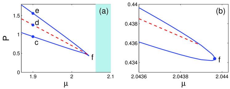
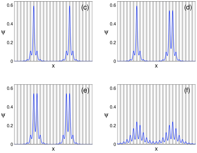
Figure 2: (a) Numerical power curve for bound states involving two solitary waves of the same envelope polarity with $N=10$ and $\sigma=1$ (self-focusing nonlinearity); the shaded region is the first Bloch band. (b) Amplification of (a) near the bifurcation point. (c–f) Soliton profiles at points of the power curve marked by the same letters in (a). Shaded stripes represent lattice sites (locations of low potentials); stripe separation is equal to the potential period, $\pi$.

Next, we turn to quantitative comparison between the analysis and numerics. For this purpose, we choose to consider bound states comprising solitary waves with opposite envelope polarity (the results of comparison for bound states with same envelope polarity are very similar). Specifically, once again, we assume self-focusing nonlinearity ($\sigma=1$) and take $N=10$, but the envelopes of the two solitary waves in the bound state now have opposite polarity. Figure 3a displays the numerical power diagram near the bifurcation point $\mu_{c}=2.04442$, and figure 3b illustrates the analytical power curves given by (48) and (49) near the analytical bifurcation point $\mu_{c}=\mu_{0}-\epsilon_{c}^{(1)2}=2.04446$, where $\epsilon_{c}^{(1)}=0.1368$ as obtained from equation (32). (To compute the analytical power curves, we first solve equations (28) for $\delta$ as a function of $\epsilon$ for $\epsilon_{c}^{(1)}<\epsilon\ll 1$, and then use $\epsilon=\sqrt{|\mu_{0}-\mu|}$.) Both the numerical and analytical power curves in figure 3a,b exhibit three branches, as expected. In addition, the middle (mixed-site) branch now bifurcates from the lower-power (on-site) branch, again in agreement with the analysis in the end of §5. Quantitatively, the numerical and analytical power curves are also in reasonable agreement, especially considering that the analytical bifurcation point here is $\epsilon_{c}^{(1)}=0.1368$, which is not all that small; moreover, for this value of $\epsilon$ and $N=10$, $\epsilon S\sim 4$, which is not all that large. Figure 3c,d shows quantitative comparison of numerics and analysis for the bound-state profiles on the lower- and higher-power branches at $\mu=2.0438$ (near the bifurcation point). The corresponding analytical bound-state profiles (red dashed curves) are given by (37). Here, the locations of the two solitary waves involved in the bound state, namely, $x_{0}^{\pm}$, are determined by (35); these values are dependent on $\delta(\epsilon)$, which is found by solving equations (28) with $\epsilon=\sqrt{|\mu_{0}-\mu|}$. The analytical solution profiles show good agreement with the numerical ones.

   

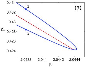
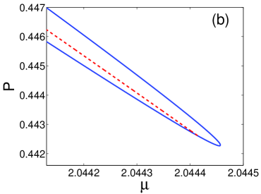
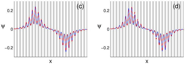
Figure 3: (a,b) Power curves for bound states involving two solitary waves with opposite envelope polarity and $N=10$, for self-focusing nonlinearity ($\sigma=1$): (a) numerical; (b) analytical. The analytical solid blue branches are obtained from equations (48) and (28a), while the analytical dashed red branch is obtained from equations (49) and (28b). (c,d) Soliton profiles at the points (corresponding to $\mu=2.0438$) of the lower and upper branches marked by the same letters in (a). Solid blue curves: numerical; dashed red curves: analytical as given by (37). (Online version in colour.)

As another quantitative comparison, we examine the dependence of the bifurcation point $\epsilon_{c}^{(1)}$ on the parameter $N$ that controls the separation distance of the two solitary waves in a bound state. The analytical and numerical values of this bifurcation point against $N$ are displayed in figure 4 for solitons with the same as well as opposite envelope polarities and self-focusing nonlinearity ($\sigma=1$). Here, the analytical bifurcation point $\epsilon_{c}^{(1)}$ is obtained from solving equation (32), and this value is the same for both cases of envelope polarity (with the same $N$). For both envelope polarities, the numerical values for $\epsilon_{c}^{(1)}$ approach the analytical ones when $N\to\infty$, confirming the asymptotic accuracy of our analysis.

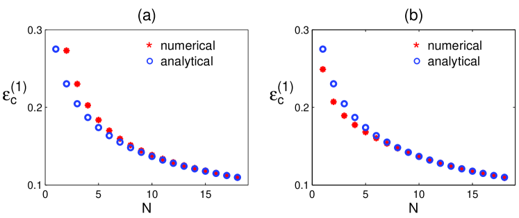
Figure 4: Comparison between analytical and numerical values of the bifurcation point $\epsilon_{c}^{(1)}$ at various values of $N$ for $\sigma=1$ (self-focusing nonlinearity): (a) same envelope polarity; (b) opposite envelope polarity. The analytical $\epsilon_{c}^{(1)}$ is obtained by solving equation (32).

As a final comparison, we assume self-defocusing nonlinearity ($\sigma=-1$) and consider bound states involving solitary waves with the same envelope polarity. For $N=10$, the numerical results for this family of bound states are displayed in figure 5. The power curve features three branches (figure 5a), and the middle branch bifurcates from the upper branch (figure 5b), in agreement with the asymptotic analysis. In addition, the bound state at point c on the lower branch comprises two on-site solitons which are separated by $(N+1)\pi=11\pi$ (see figure 5c), and the bound state at point d on the upper branch comprises two off-site solitons which are separated by $N\pi=10\pi$, again consistent with the previous analysis. It may seem puzzling at first sight that the two on-site solitons in figure 5c are of opposite signs, given that the envelopes of these solitons ought to have the same polarity. To explain this feature, note that at the band edge relevant here, $\mu_{0}=2.266735$, which is the upper edge of the first Bloch band, the Bloch mode $p(x)$ is $2\pi$-periodic, and its adjacent peaks have opposite signs, similar to the function $\cos x$ (see Yang 2010, $\S 6.1.1$). Since the two on-site gap solitons in figure 5c are separated by $(N+1)\pi=11\pi$, the Bloch function $p(x)$ at the centres of these solitons then has opposite sign. Thus, even though the envelopes of the two gap solitons have the same polarity, the overall gap-soliton profiles, which are products of the Bloch function and the envelope function, have opposite sign, as in figure 5c.

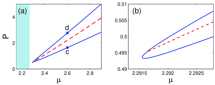
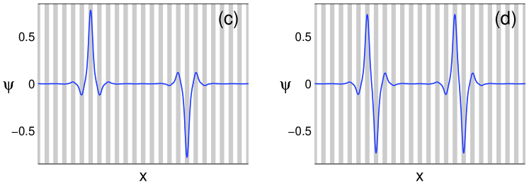
Figure 5: (a) Numerical power curve for bound states involving solitary waves of the same envelope polarity with $N=10$ and $\sigma=-1$ (self-defocusing nonlinearity); the shaded region is the first Bloch band. (b) Amplification of (a) near the bifurcation point. (c,d) Bound-state profiles at points of the power curve marked by the same letters in (a).

7 Concluding remarks

In this paper, an asymptotic theory was developed for stationary gap-soliton bound states consisting of two fundamental gap solitons in 1D periodic media. It was shown that there is a countable set of such bound state families, characterized by the separation distance of the two solitary waves involved, and each family features three distinct solution branches that bifurcate near band edges at small, but finite, amplitude. Of these three solution branches, one branch contains bound states whose fundamental solitons are both on-site; the second branch contains bound states whose fundamental solitons are both off-site; and the third branch represents bound states in which one fundamental soliton is on-site and the other off-site. The power curves associated with these solution branches were computed asymptotically for large solitary-wave separation. On the power diagram, the on-site solution branch is always the lower-power branch, the mixed-site branch the middle branch, and the off-site branch is the higher-power branch; in addition, the middle branch bifurcates from the upper (lower) branch when the envelopes of the two fundamental solitons in the bound state have the same (opposite) polarity. These analytical results were compared with numerical results and good agreement was obtained.

There are several common features between the results of this article and those obtained by Yang & Akylas (1997) for two-wavepacket bound states in the fifth-order KdV equation. In that case, a countable set of bound states also bifurcate at finite values of the wave amplitude, and each solution family also features multiple branches, with asymmetric-wave branches bifurcating off symmetric-wave branches. Furthermore, the techniques for constructing bound states in these two models follow along the same lines. Even though the current lattice model (4) is not translation invariant, while the fifth-order KdV equation is, remarkably, both models admit very similar classes of solitary-wave solutions.

In addition to being of fundamental interest, the bound states discussed here could also prove useful in applications as they allow increased flexibility in the profiles of localized nonlinear modes within band gaps. In a recent demonstration of image transmission in photonic lattices, in fact, Yang et al. (2011) utilized 2D higher-order gap solitons of various shapes, and those gap solitons are closely related to the 1D bound states constructed in the present paper. For the purpose of assessing the potential usefulness of these 1D bound states, of course, it is necessary to examine the stability properties of the various bound-state families, a question that will be taken up in future studies.

In this paper, attention was focused on bound states consisting of only two fundamental gap solitons; extending the analysis to more complicated bound states involving three or more fundamental solitons, as well as to bound states in 2D periodic media, will be left to future studies.

Our final remark is that, since the bound states constructed in this paper bifurcate near Bloch-band edges at finite amplitude, their power curves always terminate before band edges and never reach them (see figures 2a and 5a). This feature of the power curve is shared by some other types of gap solitons, such as the truncated-Bloch-wave solitons (Alexander et al. 2006; Yang 2010). Whether the present analysis can be applied to those gap solitons needs further investigation.