Soliton on Unstable Condensate

Abstract

We construct new exact solutions of the focusing Nonlinear Schrödinger equation (NLSE). This is a soliton propagating on an unstable condensate. The Kuznetsov and Akhmediev solitons as well as the Peregrine instanton are particular cases of this new solution. We discuss applications of this new solution to the description of freak (rogue) waves in the ocean and in optical fibers.

–Introduction – This research was motivated by intention to develop an analytic theory of freak (or rogue) waves in ocean and optic fibers. In the recent time the simplest and most universal model for description of these waves is the focusing NLSE (Nonlinear Schrödinger Equation). In application to the theory of ocean waves this equation is used since 1968  Zakharov1968 . In nonlinear optics it was known even earlier  Townes1964 .

The focusing NLSE is the model of the first approximation only. For the surface of fluid this model describes the essentially weakly nonlinear quasimonochromatic wave trains with average steepness not more than $5\cdot 10^{-2}$ only  Dyachenko2008 . In nonlinear optics its application is also limited to the case of waves of small amplitudes (see, for instance  Kivshar-Agraval2003 ). Nowadays a lot of models specializing the NLSE are developed. For the surface waves these are Dysthe equations  Dysthe-Trulsen1999 ; Zakharov-Dyachenko2010 , for the waves in optic fibers are equations that include the third time derivatives and more complex forms of nonlinearity (see for instance  Zakharov-Kuznetsov1998 ; Balakin2007 ). Also, freak waves in the ocean were studied by numerical modeling of exact Euler equations for potential flow with free boundary  Zakharov-Dyachenko-Prokofiev2006 ; Chalikov-Sheinin2005 . The behavior of freak waves studied by NLSE and by more sophisticated models shows considerable quantitative difference. Nevertheless, advanced improvement of NLSE does not lead to any qualitatively new effects. That means that a careful and detailed study of NLSE solutions is still very important problem.

It has been known since 1971 that the focusing NLSE is a very special system, integrable by the Inverse Scattering Method  Zakharov-Shabat1972 . Since that time hundreds of articles have been devoted to this subject (see for instance the monographs  Faddeev-Takhtajan2007 ; Sulem-Sulem1999 ; Kharif-Pelinovsky2009 . In spite of great attention to this field, solutions of focusing NLSE in the presence of an unstable condensate have not been studied thoroughly enough. However, this case is the most interesting for developing a theory of freak waves, because there is now universal agreement that extreme waves appear as a result of modulation instability of quasimonochromatic nonlinear waves. A nonlinear theory describing the development of unstable condensate in the frame of 1-D focusing NLSE has not yet been formulated. Moreover, even ordinary solitonic solutions propagating over unstable condensate have not yet been found.

Some special cases are already known. In the presence of condensate the maximally analytic wave function of auxiliary linear Zakharov-Shabat operator has, in the right half-plane of the complex variable $\lambda=i\eta$ (where $\eta$ is the spectral parameter), an additional cut on the real axis up to the point $\lambda=A$ (here $A$ is the condensate amplitude). The soliton adds a simple pole to the wave function singularity. Only the cases when the pole is on the real axis have been studied. In 1978 Kuznetsov  Kuznetsov1977 found an important solitonic solution with the pole outside of the cut $Re\lambda>A$. This solution is a standing soliton with a changing amplitude. Later on this solution was rediscovered by other authors  Kawata1978 ; Ma1979 . In 1983 Peregrine Peregrine1983 found a solution with the pole exactly at the branch point. This is a remarkable instanton homoclinic solution - the localized events appear from the condensate and return back to it. Now there are already known multi-instanton solutions  Matveev2010 ; Matveev2011 . The importance of these solutions for the development of the theory of freak waves is stressed in the article  Shrira2010 . Then, the solution of Akhmediev with co-authors is widely known  Akhmediev1986 . This solution corresponds to the pole posed inside the cut and is periodic in space but local in time. Unlike the Peregrine instanton, this solution change the condensate phase.

In this article we describe a general solitonic solution with the pole at an arbitrary point in the complex upper half-plane of the spectral parameter. This solution includes all other known cases and changes the condensate phase. It is a moving localized soliton with periodic nonmonochromatic intrinstic structure. When the pole is far away from the cut, but close to real axis, the solution is similar to Kuznetsov’s soliton. However, when approaching the cut (but still not on the real axis) the velocity of soliton propagation and the size of soliton tend to infinity, so the Akhmediev limit happens to be very singular.

For constructing this solution we use the advanced mathematical technique of the ”local $\overline{\partial}$ - problem”. This method is a modernization of the ”dressing method”, described in  Zakharov-Shabat1979 ; Zakharov-Manakov-Novikov-Pitaevskii1984 .

–NLSE via local matrix $\overline{\partial}$ problem – We study solutions of the following NLSE

$$i\varphi_{t}-\frac{1}{2}\varphi_{xx}-(|\varphi|^{2}-A^{2})\varphi=0$$ (1)

with boundary conditions $|\varphi|^{2}\rightarrow A^{2}$ at $x\rightarrow\pm\infty$. Here $A=\overline{A}$ is a real constant. Equation (1) is the compatibility condition for the following overdetermined linear system for a matrix function $\Psi$:

$$\frac{\partial\Psi}{\partial x}=\widehat{U}\Psi,\;\;i\frac{\partial\Psi}{\partial t}=(\lambda\widehat{U}+\widehat{W})\Psi$$ (2)

Here

$$\widehat{U}=I\lambda+u$$

$$I=\begin{pmatrix}1&0\\ 0&-1\end{pmatrix},\;\;u=\begin{pmatrix}0&\varphi\\ -\overline{\varphi}&0\end{pmatrix}$$

$$\widehat{W}=\frac{1}{2}\begin{pmatrix}|\varphi|^{2}-|A|^{2}&\varphi_{x}\\ \overline{\varphi}_{x}&-|\varphi|^{2}+|A|^{2}\end{pmatrix}$$ (3)

If $\varphi=0$, system (2) has the following solution:

$$\Psi_{0}=\frac{1}{\sqrt{1-q^{2}}}\begin{pmatrix}e^{\phi}&q\cdot e^{-\phi}\\ q\cdot e^{\phi}&e^{-\phi}\end{pmatrix}$$ (4)

Here

$$\phi=kx+\Omega t,\;\;k^{2}=\lambda^{2}-A^{2}$$

$$\Omega=-i\lambda k,\;\;q=-\frac{A}{\lambda+k}$$

In what follows we assume that $k\rightarrow\lambda$ at $|\lambda|\rightarrow\infty$. Then

$$\Psi_{0}^{-1}=\frac{1}{\sqrt{1-q^{2}}}\begin{pmatrix}e^{-\phi}&-q\cdot e^{-\phi}\\ -q\cdot e^{\phi}&e^{\phi}\end{pmatrix}$$ (5)

Notice that

$$\overline{k}(-\overline{\lambda})=-k(\lambda),\;\;\;\;\overline{q}(-\overline{\lambda})=-q(\lambda),\;\;\;\;\overline{\phi}(-\overline{\lambda})=\phi(\lambda)$$

and

$$\Psi^{-1}_{0}(-\overline{\lambda})=\Psi^{+}(\lambda)$$ (6)

We consider the $\overline{\partial}$-problem on the complex $\lambda$-plane. We are looking for a second order matrix $\chi(\lambda,\overline{\lambda},x,t)$ obeying the equation

$$\frac{\partial\chi}{\partial\overline{\lambda}}=\chi\cdot f(\lambda,\overline{\lambda},x,t)$$ (7)

and normalized by condition $\chi\rightarrow 1$ at $|\lambda|\rightarrow\infty$. Here

$$f=\psi_{0}f_{0}(\lambda,\overline{\lambda})\psi_{0}^{-1}$$

$$f_{0}(\lambda,\overline{\lambda})=f^{+}_{0}(\lambda,\overline{\lambda})$$ (8)

By virtue of (6) function $f$ satisfies condition $f(\lambda,\overline{\lambda})=f^{+}(\lambda,\overline{\lambda})$. This proves that

$$\chi^{-}(\lambda)=\chi^{+}(-\overline{\lambda})$$ (9)

The function $\chi$ has an asymptotic expansion at $\lambda\rightarrow\infty$

$$\chi=1+\frac{R}{\lambda}+\cdots$$ (10)

By virtue of (8) $R^{+}=R$. The function $\chi$ satisfies the following system of equations

$$\frac{\partial\chi}{\partial x}=\widehat{U}\chi-\chi\widehat{U}_{0}$$

$$i\frac{\partial\chi}{\partial t}=(\lambda\widehat{U}+\widehat{W})-\lambda\chi\widehat{U_{0}}$$ (11)

Here $\widehat{U}$ and $\widehat{W}$ are given by expressions (3). Because system (11) is overdeterminated, we have the following expression for $\varphi$:

$$\varphi=A-2R_{(12)}$$ (12)

For an arbitrary choice of matrix function $f_{0}(\lambda,\overline{\lambda})$ satisfying condition (8), function $\varphi$ is the solution of equation (1).

–Solitonic solution – Let us choose

$$f_{0}(\lambda,\overline{\lambda})=\begin{pmatrix}0&\alpha(\lambda,\overline{\lambda})\\ \overline{\alpha}(-\overline{\lambda},-\lambda)&0\end{pmatrix}$$

The function $f$ now takes the form:

$$f(\lambda,\overline{\lambda},x,t)=\alpha e^{2\phi}A+\overline{\alpha}(-\overline{\lambda},-\lambda)Be^{-2\phi}$$

The matrices $A,B$ are degenerate

$$A_{\alpha\beta}=a_{\alpha}b_{\beta},\;\;B_{\alpha\beta}=c_{\alpha}d_{\beta}$$

$$a=(1,q),\;\;b=(-q,1);\;\;\;\;c=(q,1),\;\;d=(1,-q)$$

and

$$(\overrightarrow{a}\cdot\overrightarrow{b})=a_{\alpha}b_{\alpha}=0,\;\;\;\;\;\;\;\;\;\;\;\;(\overrightarrow{c}\cdot\overrightarrow{d})=c_{\alpha}d_{\alpha}=0$$

We now choose

$$\alpha(\lambda,\overline{\lambda})=C\delta(\lambda-\eta)$$

Here $\delta(\lambda-\eta)$ is the two-dimensional $\delta$-function. Later on, the existence of $\delta$-function allows us to work with two values of function $\phi$:

$$\phi(\eta)=k(\eta)(x-i\eta t),\;\;\phi(-\overline{\eta})=-\overline{\phi}$$

We now assume that $q(\eta)=q$, $q(-\overline{\eta})=-\overline{q}$. In a neighborhood of $\lambda=\eta$, $\lambda=-\overline{\eta}$ we expand A and B:

$$A=A_{0}+A_{1}(\lambda-\eta),\;\;B=B_{0}+B_{1}(\lambda+\overline{\eta})$$

$$A_{0}=\begin{pmatrix}-q&1\\ -q^{2}&q\end{pmatrix},\;\;B_{0}=\begin{pmatrix}q&-q^{2}\\ 1&-q\end{pmatrix}$$

$$A_{1}=-\frac{q}{k}\begin{pmatrix}1&0\\ -2q&0\end{pmatrix},\;\;B_{1}=-\frac{\overline{q}}{\overline{k}}\begin{pmatrix}-1&-2\overline{q}\\ 0&1\end{pmatrix}$$

Note that now $\overrightarrow{c}=\overrightarrow{b^{*}}$ and $\overrightarrow{d}=\overrightarrow{a^{*}}$. We will find a solution of the $\overline{\partial}$ - problem (7) in the form of rational functions with two poles:

$$\chi=1+\frac{U}{\lambda-\eta}+\frac{V}{\lambda+\overline{\eta}}$$ (13)

where $U$, $V$ are constant degenerate matrices:

$$U_{\alpha\beta}=u_{\alpha}b_{\beta},\;\;V_{\alpha\beta}=v_{\alpha}a^{*}_{\beta}$$

To avoid a singularity we require

$$UA_{0}=0,\;\;VB_{0}=0$$

Substituting (13) into (7) we end up with a simple linear system of equations for $u_{\alpha}$ and $v_{\alpha}$:

$$u_{\alpha}(1+\frac{q}{k}Ce^{2\phi})-\frac{1+|q|^{2}}{\eta+\overline{\eta}}Ce^{2\phi}v_{\alpha}=a_{\alpha}Ce^{2\phi}$$

$$\frac{1+|q|^{2}}{\eta+\overline{\eta}}Ce^{2\overline{\phi}}u_{\alpha}+(1+\frac{\overline{q}}{\overline{k}}\overline{C}e^{2\overline{\phi}})v_{\alpha}=\overline{b}_{\alpha}\overline{C}e^{2\overline{\phi}}$$

By virtue of (15) the solution of equation (1) is given as follows

$$\varphi=A-2(u_{1}+v_{1}\overline{q})$$

It is convenient to present final answer in terms of a uniformizing variable $\xi$:

$$\lambda=\frac{A}{2}(\xi+\frac{1}{\xi}),\;\;k=\frac{A}{2}(\xi-\frac{1}{\xi}),\;\;\xi+\overline{\xi}\neq 0$$

Then $\xi=Re^{-i\alpha}$. Now:

$$\phi=\frac{1}{2}(\ae x-\gamma t)+i\frac{1}{2}(kx-\omega t)$$

Here

$$\ae=A(R-\frac{1}{R})\cos(\alpha),\;\;\gamma=-\frac{A^{2}}{2}(R^{2}+\frac{1}{R^{2}})\sin(2\alpha)$$

$$k=A(R+\frac{1}{R})\sin(\alpha),\;\;\omega=\frac{A^{2}}{2}(R^{2}-\frac{1}{R^{2}})\cos(2\alpha)$$

After the proper choice of $C$ we finish with

$$\varphi=\frac{Ae^{2i\alpha}}{2}\biggl{(}\frac{2\cos(2\alpha)\cosh(u+w)-\frac{1}{a}(R^{2}+\frac{1}{R^{2}})\cos(v)}{\cosh(u+w)-\frac{1}{a}\cos(v)}+$$

$$i\frac{2\sin(2\alpha)\sinh(u+w)+(R^{2}-\frac{1}{R^{2}})\sin(v)}{\cosh(u+w)-\frac{1}{a}\cos(v)}\biggr{)}$$

Here

$$u=\phi+\phi^{*}=\ae x-\gamma t,\;\;v=\phi-\phi^{*}=i(kx-\omega t)$$

$$a=\frac{1+R^{2}}{2R\cos(\alpha)},\;\;w=\ln(a)$$

Note that

$$\varphi\rightarrow A\;\;\;\;\;\text{at}\;\;\;x\rightarrow-\infty$$

$$\varphi\rightarrow Ae^{4i\alpha}\;\;\;\;\;\text{at}\;\;\;x\rightarrow+\infty$$

$$|\varphi|^{2}=A^{2}\;\;\;\;\;\text{at}\;\;\;x\rightarrow\pm\infty$$

Fig. 1 show a typical solitonic solution at the moment of maximum and minimum amplitude.

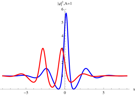
Figure 1: Typical solitonic solution at the moment of maximum (blue) and minimum (red) of amplitude. ($R=2,\alpha=\frac{5}{16}\pi$)

In our notation, we obtain Kuztensov’s solution in the case of real $\xi$. When the pole is near the real axis, our solution looks like a Kuznetsov soliton moving with constant speed. This speed tends to zero in the limit $Im(\xi)\rightarrow 0$. Thus, there is a broad area of Kuznetsov-like solutions near the real $\xi$ axis. Fig. 2 shows a typical solution corresponding to this case. The blue curve corresponds to the moment of maximum value of $|\varphi|^{2}$, while the red one corresponds to its minimal value.

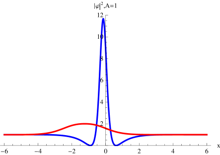
Figure 2: Kuznetsov-like solution at the moment of maximum (blue) and minimum (red) of amplitude ($R=2,\alpha=\frac{\pi}{12}$).

The Akhmediev case appears for $|\xi|^{2}=1$. Near this area the solution is a wave train moving with constant speed and without changing its shape. We obtain the approximate expression for the envelope $s(x,t)$ of this wave train in the case of $Arg(\xi)=\frac{\pi}{4}$:

$$|s|^{2}=A\biggl{(}1+Q\frac{\cosh(u+w)}{(a^{2}\cosh^{2}(u+w)-4)^{\frac{3}{2}}}\biggr{)}$$ (15)

Here

$$Q=a(6+R^{4}+\frac{1}{R^{4}}-4a^{2})$$

For an arbitrary value of $Arg(\xi)$ the envelope $s$ behaves similarly but the expression for it is more complicated. Fig. 3 shows a typical solitonic solution near $|\xi|^{2}=1$ and its envelope as calculated by (15).

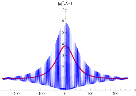
Figure 3: Soliton and its envelope. ($R=1.01,\alpha=\frac{\pi}{4}$)

The speed and size of the wave train increases without bound in the limit case when $\xi$ tends to the circle $|\xi|^{2}=1$. Thus the Akhmediev solution can be understood as a special case when the size and speed of the wave train tends to infinity.

Using the presented method one can construct multisoliton solutions with different values $\xi_{1},..,\xi_{n}$ of the uniformizing parameter $\xi$. By taking all $\xi_{i}\rightarrow 1$ one can obtain ”multi-instanton” solutions found recently in articles  Matveev2010 ; Matveev2011 .

–Conclusion – We have discovered new solitonic solutions of the NLSE. This discovery essentially increases the number of candidate solutions for the analytic description of rogue waves. We expect that similar solutions exist in more exact models than NLSE. Since the found solutions change the condensate phase they can hardly be used for this purpose directly. However, the two-soliton solutions with complex conjugated values of poles ($\eta,\overline{\eta}$) are relevant candidates which could compete with homoclinic instanton-like solutions.

- (1) V. E. Zakharov, J. Appl. Mech. and Tech. Phys. 9(2), 190 (1968)
- (2) R. Y. Chiao, E. Garmire and C. H. Townes, Phys. Rev. Lett. 13, 479 (1964)
- (3) A. I. Dyachenko and V. E. Zakharov, JETP Lett. 88, 356 (2008)
- (4) Y. S. Kivshar, G. Agrawal, Optical Solitons: From Fibers to Photonic Crystals (Academic Press, 2003)
- (5) K. B. Dysthe, K. Trulsen, Phys. Scripta 82, 48 (1999)
- (6) V. Zakharov and A. Dyachenko, Eur. J. Mech. B/Fluids 29, 127 (2010)
- (7) V. E. Zakharov and E. A. Kuznetsov, JETP. 86(5), 1035 (1998)
- (8) A. A. Balakin, A. G. Litvak, V. A. Mironov and S. A. Skobelev, JETP. 104(3), 363 (2007)
- (9) V. E. Zakharov, A. I. Dyachenko, A. O. Prokofiev, Eur. J. of Mech. B/Fluids 25(5), 677 (2006)
- (10) D. Chalikov, D. Sheinin, Journ. Comp. Phys. 210, 247 (2005)
- (11) V. E. Zakharov and A. B. Shabat, Sov. Phys. JETP 34(1), 62 (1972)
- (12) L. D. Faddeev and L. A. Takhtajan, Hamiltonian Methods in the Theory of Solitons (Springer-Verlag, Berlin, Heidelberg, 2007)
- (13) C. Sulem and P-L. Sulem, The nonlinear schrodinger equation. (Self focusing and wave collapse) (Springer-Verlag, New York, Berlin, Heidelberg ,1999)
- (14) C. Kharif, E. Pelinovsky and A. Slunyaev, Rogue Waves in the Ocean (Springer ,2009)
- (15) E. A. Kuznetsov, Solitons in a parametrically unstable plasma, Sov. Phys. - Dokl. (Engl. Transl.) 22, 507 (1977). On solitons in parametrically unstable plasma, Doklady USSR (in Russian) 236, 575 (1977)
- (16) T. Kawata and H. Inoue, J. Phys. Soc. Jpn. 44, 1722 (1978)
- (17) Y.-C. Ma, Stud. Appl. Math. 60, 43 (1979).
- (18) D. H. Peregrine, J. Aust. Math. Soc. Series B 25, 16 (1983)
- (19) P. Dubard, P. Gaillard, C. Klein, V.B. Matveev, Eur. Phys. J. Special Topics 185, 247 (2010).
- (20) P. Dubard, V.B. Matveev, Nat. Hazards. Earth. Syst. Sci. 11, 667 (2011)
- (21) V. I. Shrira and V. V. Geogjaev, J. Eng. Math. 67, 11 (2010).
- (22) N. N. Akhmediev and V. I. Korneev, Theor. Math. Phys. (USSR) 69, 1089 (1986).
- (23) V. E. Zakharov and A. B. Shabat Funct. Anal. Appl. 13(3), 166 (1979)
- (24) V. E. Zakharov, S. V. Manakov, S. P. Novikov and L. P. Pitaevskii, Theory of solitons. The inverse scattering method (Plenum Press, New York, London ,1984)