From microscopic taxation and redistribution models
to macroscopic income distributions

Abstract

We present here a general framework, expressed by a system of nonlinear differential equations, suitable for the modelling of taxation and redistribution in a closed society. This framework allows to describe the evolution of the income distribution over the population and to explain the emergence of collective features based on the knowledge of the individual interactions. By making different choices of the framework parameters, we construct different models, whose long-time behavior is then investigated. Asymptotic stationary distributions are found, which enjoy similar properties as those observed in empirical distributions. In particular, they exhibit power law tails of Pareto type and their Lorenz curves and Gini indices are consistent with some real world ones.

1 Introduction

The interest of physicists and mathematicians towards complex systems arising in social and economical sciences has been constantly growing in the last years, as attested by the number of published papers. Among the subjects these papers deal with, one finds opinion formation dynamics (see for example [2, 5, 6, 13, 21]), relaxation processes to steady wealth and income distributions [7, 8, 9, 10, 11, 12, 18], mechanisms of financial markets and other out-of-equilibrium economic and financial phenomena [1, 15, 19, 20]. These topics share the common fact of referring to systems (populations) composed by a large number of interacting elements (individuals). And this is why methods and tools from statistical mechanics and kinetic theory have been and are being adapted and employed to investigate them.

In a recent paper, [4], one of the present authors introduced a general framework, suitable for the construction of models of taxation and redistribution in a closed society. This framework originates from a discrete active particle kinetic approach [3] and is expressed by a system of nonlinear ordinary differential equations. The equations are as many as the classes, each one characterized by its “average income”, in which the population can be divided. Each equation gives the variation in time of the fraction of individuals belonging to a certain class. The framework provides a description of the evolution of the wealth distribution over the population and aims at explaining emerging collective features, based on the knowledge of the individual interactions. As a case study, also a specific model was formulated in [4]. To this end, the general mathematical framework was exploited and a particular choice for the values of some of its parameters was made. The well-posedness of the model as well as the existence of two conserved quantities, corresponding to the total population and the global wealth, was then established. Several simulations were carried out for the case in which the number $n$ of income classes (and of differential equations) is equal to $5$. Specific attention was devoted in [4] to the differences, detectable from the shape of the long-time income distributions, among systems with different taxation rates. The result was that increasing the difference between the maximum and the minimum tax rate leads, at the asymptotic equilibrium, to the growth of the middle classes, to the detriment of the poorest and the richest classes. This is a reasonable feature which encourages, in spite of the naiveness and roughness of the model, a thorough investigation. A natural observation is that the study of the model in the particular case with 5 income classes does not allow for example to recover the Pareto-law which is observed in real world economies. As a matter of fact, $n=5$ is too small a number for a tail of the steady income distribution to show up. In view of that, we started performing a great deal of computational simulations relative to the model with greater values of $n$. We tried and considered several choices of the model parameters, expressing e.g. different characterizations of the incomes or of the tax rates. With the aim of treating reasonable cases, as far as possible comparable with real world ones, we focused our attention on “realistic”initial population distributions, where the majority of individuals belongs to lower income classes, while higher classes are less densely populated (see Section $3$ for details). The numerical solutions systematically show that for any fixed value of the total wealth a unique asymptotic stationary distribution exists, independently of the random choice of the initial population distribution (subjected only to the just mentioned “realistic”requirement). The asymptotic stationary distribution exhibits the following patterns: the density of the low income classes is smaller than for the low-medium classes, the maximal density is achieved by the low-medium classes and the density progressively decreases for the higher income classes. In fact, the asymptotic distributions exhibit salient features of empirical distributions (see e.g. [22, page $14$], [23, page $19$], and [24, page $8$]). At a closer look, one also finds that the tails of the distributions have indeed a power law behavior [16]. An analysis of the shape of the tails and its relation with the parameters of the model is the subject of the present paper.

The paper is organized as follows. In Section $2$, we review for the convenience of the reader the framework and the model introduced in [4]. Section $3$ focuses on the existence of asymptotic stationary distributions and on their properties. In particular, Pareto tails [17] are found to occur and their Pareto indices are calculated in some different cases. The last section provides a short summary of the content of the paper and a brief mention of possible future developments.

Before starting, it may be of interest comparing certain features of our models with those of others available in the econophysics or “classical”mathematical economics literature. Some immediately evident differences concern the mathematical formulation of the income distribution problem. A first class of works (see [18] for a review) develop a statistical analysis of the population by means of Montecarlo simulations of the interactions of a large number of individuals. In these models the interaction rules can be defined with great freedom, because they are applied in a straightforward way through the simulation algorithm. At the same time, the method is not based upon evolution equations. Therefore it lacks general mathematical theorems which should keep account of specific hypotheses on the interactions. To draw a comparison, within our framework we are free to fix several parameters (interaction frequency, taxation rates, etc.), but for the models to be conservative, some terms in the transition probabilities expressing income class changes must be proportional to the reciprocal of the income difference $|r_{i}-r_{j}|$. If one changes this dependence, supposing for instance that the transition probability is proportional to the reciprocal of $|r_{i}-r_{j}|^{2}$, then the conservation of the total wealth ceases to be valid. The dependence of the model on the details of the interactions is also typical of the approaches based on the Boltzmann equation [11, 12]. In the application of this equation to the kinetic theory of gases the interactions are determined to a large extent by physical conservation laws and symmetry principles. In the applications to econophysics there is some more freedom as for the definition of the interactions. Within this approach it is possible proving powerful general results concerning the moments of the distribution function $f(w,t)$ and the Pareto index of the stationary asymptotic distribution. It has to be noticed however that the structure of the Boltzmann equation requires advanced mathematical tools for his treatment: the partial time derivative of the income distribution function $f(w,t)$ is given by an integral operator acting on $f(w,t)$ and also involves an average on some stochastic variables. The time evolution is usually computed through some approximate discretization method. Similar approximations are also employed in the classical economics theory [14]. There, the time evolution equations are not derived from hypotheses on the “microscopic”interactions, but from variational principles and other general “macroscopic”considerations. Of course, the classical approach is characterized by a more realistic description of the dynamics of a complex economy, taking into consideration also different kinds of assets, financial transactions, government intervention etc.. Our framework introduces from the beginning a discretization of the distribution function. We suppose that the individuals belong to income classes and pass from one class to another with certain probabilities. In our case, the equivalent of the classical distribution function could be written as a liner combination of Dirac delta-functions:

$$f(w,t)=\sum_{i}x_{i}(t)\delta(w-r_{i})\,.$$

The quantities which evolve in time are discrete, like the individuals in a Montecarlo simulation, but in fact they express already averages, weighed with certain probabilities, much like the matrix elements of a wavefunction in quantum mechanics. The formalism is familiar to physicists, since it reminds of the Schroedinger equation of an atomic system expanded on a basis of states. This approach was previously devised to describe problems of opinion formation [5, 6], for which the state of an individual can be reasonably represented by a discrete rather than real variable. It provides some advantages, however, also for the treatment of income distributions. It allows, for instance, a very natural definition of different taxation rates for different income classes, and a division of the population in classes with incomes that increase non-linearly. In turn, this enables a better representation of the ”super-rich” classes in a population.

2 Taxation and redistribution in a closed trading market society

In this section we shortly describe the general mathematical framework introduced in [4] for the modelling of the dynamical process of taxation and redistribution in a closed trading market society. We then construct a particular family of models, by attributing specific values to the parameters in the framework.

2.1 A general framework

Before writing down the system of nonlinear ordinary differential equations which constitute the framework, we briefly describe the context and introduce some notation.

Consider a population of individuals belonging to a finite number $n$ of classes, each one characterized by its “average income”. Let $r_{1},r_{2}\ldots r_{n}$ denote the average incomes of the $n$ classes, ordered so that $r_{1}\leq r_{2}\leq\ldots\leq\ r_{n}$, and let $x_{i}(t)$, where $x_{i}:{\bf R}\to[0,+\infty)$ for $i\in\Gamma_{n}=\{1,2,...,n\}$, denote the fraction at time $t$ of individuals belonging to the $i$-th class. In the following, the indices $i,j,h,k$, etc. will always belong to $\Gamma_{n}$.

What produces the dynamics is a whole of pairwise interactions of economic nature, subjected to taxation. Call $S$ the fixed amount of money that people may exchange during their interactions.

Any time an individual of the $h$-th class has to pay a quantity $S$ to an individual of the $k$-th class, this one in turn has to pay some tax corresponding to a percentage of what he is receiving. This tax is quantified as $S\,\tau$, where the tax rate $\tau=\tau_{k}\leq 1$ depends in general on the class of the earning individual. Since the amount of money corresponding to the tax $S\,\tau$ should go to the government, which then is supposed to use the money collected through taxation to provide welfare services for the population, we interpret the welfare provision as an income redistribution. Ignoring the passages to and from the government, we adopt the following equivalent mechanism as the mover of the dynamics: in correspondence to any interaction between an $h$-individual and a $k$-individual, where the one who has to pay $S$ to the other one is the $h$-individual, as a matter of fact the $h$-individual pays to the $k$-individual a quantity $S\,(1-\tau)$ and he pays as well a quantity $S\,\tau$, which is divided among all $j$-individuals for $j\neq n$. Accordingly, the effect of taxation and redistribution is equivalent to the effect of a quantity of interactions between the $h$-individual and each one of the $j$-individuals for $j\neq n$, which are “induced”by the effective $h$-$k$ interaction. To fix notations, we may distinguish between “direct”interactions ($h$-$k$) and “indirect”interactions ($h$-$j$ for $j\neq n$).

Now: any direct or indirect economical interaction yields as a consequence a possible slight increase or slight decrease of the income of individuals.

To translate in mathematical terms all that, we introduce

$\bullet$ the (table of the) interaction rates

$$\eta_{hk}\in[0,+\infty)\,,$$

expressing the number of effective encounters per unit time between individuals of the $h$-th class and individuals of the $k$-th class;

$\bullet$ the (tables of the) direct transition probability densities

$$C_{hk}^{i}\in[0,+\infty)\,,$$

satisfying for any fixed $h$ and $k$

$$\sum_{i=1}^{n}C_{hk}^{i}=1\,,$$

which express the probability density that an individual of the $h$-th class will belong to the $i$-th class after a direct interaction with an individual of the $k$-th class;

$\bullet$ the (tables of the) indirect transition variation densities

$$T_{[hk]}^{i}\,:{\bf R}^{n}\to{\bf R}\,,$$

where the $T_{[hk]}^{i}(x)$ with $x=(x_{1},...,x_{n})\in{\bf R}^{n}$ are continuous functions, satisfying, for any fixed $h$, $k$ and $x\in{\bf R}^{n}$

$$\sum_{i=1}^{n}T_{[hk]}^{i}(x)=0\,.$$

These functions account for the indirect interactions and express the variation density in the $i$-th class due to an interaction between an individual of the $h$-th class with an individual of the $k$-th class.

If the interactions rates $\eta_{hk}$ are chosen for simplicity all equal to $1$, the evolution of the class populations $x_{i}(t)$ is governed by the following differential equations, in which, of course, the contribution of both direct and indirect interactions is present:

$${{dx_{i}}\over{dt}}=\sum_{h=1}^{n}\sum_{k=1}^{n}{\Big{(}}C_{hk}^{i}+T_{[hk]}^{i}(x){\Big{)}}x_{h}x_{k}-x_{i}\sum_{k=1}^{n}x_{k}\,.$$ (1)

This is a system of nonlinear ordinary differential equations. For instance, if the values of the elements $T_{[hk]}^{i}$ are chosen as in the next subsection, the r.h.s. of the equations $(\ref{evolution eq eta = 1})$ is a polynomial of third degree.

2.2 A family of models: special choices for the transition probabilities

In order to design within the general framework just discussed a specific model (or a specific family of models), we need to further characterize the expressions of the direct transition probability densities $C_{hk}^{i}$ and the indirect transition variation densities $T_{[hk]}^{i}(x)$. A conceivable choice is given next.

As done in the previous subsection, we take all the interaction rates $\eta_{hk}$ to be equal to one. This corresponds to assuming that all the encounters between two individuals occur with the same frequency, independently of the classes to which the two belong.

We represent the direct transition probability densities $C_{hk}^{i}$ as

$$C_{hk}^{i}=a_{hk}^{i}+b_{hk}^{i}\,,$$

where the term $a_{hk}^{i}$ expresses the probability density that an $h$-individual will belong to the $i$-th class after an encounter with a $k$-individual, when such an encounter does not produce any change of class and the term $b_{hk}^{i}$ expresses the density variation in the $i$-th class of an $h$-individual interacting with a $k$-individual.

Accordingly, the only nonzero elements $a_{hk}^{i}$ are

$$a_{ij}^{i}=1\,.$$

To define the elements $b_{hk}^{i}$, we introduce the matrix $P$, whose elements $p_{h,k}$ express the probability that in an encounter between an $h$-individual and a $k$-individual, the one who pays is the $h$-individual. Admitting also the possibility that to some extent the two individuals do not really interact, we have $0\leq p_{h,k}\leq 1$ and, furthermore, $p_{h,k}+p_{k,h}\leq 1$.

There is some arbitrariness in the construction of the matrix $P$. What is important is putting each element in the first row, as well as each element but the very last one in the last column, equal to zero. Indeed, since there is not a class lower than the first nor one higher than the $n$-th, we cannot admit the possibility for $1$-individuals [respectively, for $n$-individuals] to move back to a lower class [respectively, to advance, passing in a higher class]. Observing that also in the presence of interactions between individuals of the same class, the average wealth of the class itself decreases because of payment of taxes, we assume that individuals of class $1$ never pay (nor even $1$-individuals) while individuals of class $n$ can only receive money from other $n$-individuals.

An encounter between an $h$-individual and a $k$-individual, with $h\geq 2$ and $k\leq n-1$ and the $h$-individual paying, produces the elements

$$b_{hk}^{h-1}=p_{h,k}\,S\,(1-\tau_{k})\,\frac{1}{r_{h}-r_{h-1}}\,,\quad b_{hk}^{h}=-p_{h,k}\,S\,(1-\tau_{k})\,\frac{1}{r_{h}-r_{h-1}}\,,$$

$$b_{kh}^{k+1}=p_{h,k}\,S\,(1-\tau_{k})\,\frac{1}{r_{k+1}-r_{k}}\,,\quad b_{kh}^{k}=-p_{h,k}\,S\,(1-\tau_{k})\,\frac{1}{r_{k+1}-r_{k}}\,.$$

Therefore, the possibly nonzero elements $b_{hk}^{i}$ are of the form

$$b_{i+1,k}^{i} = p_{i+1,k}\,S\,(1-\tau_{k})\,\frac{1}{r_{i+1}-r_{i}}\,,$$

$$b_{i,k}^{i} = -\,p_{k,i}\,S\,(1-\tau_{i})\,\frac{1}{r_{i+1}-r_{i}}-\,p_{i,k}\,S\,(1-\tau_{k})\,\frac{1}{r_{i}-r_{i-1}}\,,$$

$$b_{i-1,k}^{i} = p_{k,i-1}\,S\,(1-\tau_{i-1})\,\frac{1}{r_{i}-r_{i-1}}\,,$$ (2)

where the expression for $b_{i+1,k}^{i}$ in $(\ref{b})$ holds true for $i\leq n-1$ and $k\leq n-1$, in the expression for $b_{i,k}^{i}$, the first addendum is effectively present only provided $i\leq n-1$ and $k\geq 2$ and the second addendum only provided $i\geq 2$ and $k\leq n-1$, and the expression for $b_{i-1,k}^{i}$ holds true for $i\geq 2$ and $k\geq 2$.

We express the indirect transition variation densities $T_{[hk]}^{i}(x)$ as

$$T_{[hk]}^{i}(x)=U_{[hk]}^{i}(x)+V_{[hk]}^{i}(x)\,,$$

where

$$U_{[hk]}^{i}(x)=\frac{p_{h,k}\,S\,\tau_{k}}{\sum_{j=1}^{n}x_{j}}{\bigg{(}}\frac{x_{i-1}}{(r_{i}-r_{i-1})}-\frac{x_{i}}{(r_{i+1}-r_{i})}{\bigg{)}}$$ (3)

represents the variation density corresponding to the advancement from a class to the subsequent one, due to the benefit of taxation and

$$V_{[hk]}^{i}(x)=p_{h,k}\,S\,\tau_{k}\,{\bigg{(}}\frac{\delta_{h,i+1}}{r_{h}-r_{i}}\,-\,\frac{\delta_{h,i}}{r_{h}-r_{i-1}}{\bigg{)}}\,\frac{\sum_{j=1}^{n-1}x_{j}}{\sum_{j=1}^{n}x_{j}}\,,$$ (4)

with $\delta_{h,k}$ denoting the Kronecker delta, accounts for the variation density corresponding to the retrocession from a class to the preceding one, due to the payment of some tax. In the r.h.s. of $(\ref{U_{[hk]}^i(x)})$ and $(\ref{V_{[hk]}^i(x)})$, $h>1$ and the terms involving the index $i-1$ [respectively, $i+1$] are effectively present only provided $i-1\geq 1$ [respectively, $i+1\leq n$].

Notice that for technical reasons, in the model under consideration, the effective amount of money paid as tax relative to an exchange of $S(1-\tau_{k})$ between two individuals and then redistributed among classes is given by $S\,\tau_{k}\,({\sum_{j=1}^{n-1}x_{j}})/{(\sum_{j=1}^{n}x_{j}})$ instead of $S\,\tau_{k}$.

As we shall see in the next subsection, a general theorem ensures that the solutions $x=(x_{1},\ldots,x_{n})$ of interest remain normalized during the evolution, i.e. $\sum_{j=1}^{n}x_{j}=1$. As a consequence, the expressions for $U_{[hk]}^{i}(x)$ and $V_{[hk]}^{i}(x)$ are simplified and we see from $(\ref{U_{[hk]}^i(x)})$ and $(\ref{V_{[hk]}^i(x)})$ that they both are linear functions of the $x_{i}$.

2.3 Existence and uniqueness of the solution, conserved quantities, non-negativity and normalization property

The well-posedness of the model was established in [4]. Precisely, it was proven there that, with the choice of parameters as in Subsection $2.2$, in correspondence to any initial non-negative and normalized condition $x_{0}$, a unique non-negative and normalized solution $x(t)$ exists. In geometrical terms, taken an initial condition $x_{0}=(x_{01},\ldots,x_{0n})\in\Sigma_{n-1}$, where

$$\Sigma_{n-1}={\Big{\{}}x=(x_{1},...,x_{n})\in{\bf R}^{n}:x_{i}\geq 0\ \hbox{for any}\ i\in\Gamma_{n}\ \hbox{and}\ \sum_{i=0}^{n}x_{i}=1{\Big{\}}}$$ (5)

denotes the “$(n-1)$-simplex”, a unique solution $x(t)=(x_{1}(t),\ldots,x_{n}(t))$ of $(\ref{evolution eq eta = 1})$ exists, which is defined for all $t\in[0,+\infty)$ and satisfies $x(0)=x_{0}$. Moreover,

$$x(t)\in\Sigma_{n-1}\quad\hbox{for all}\ t\geq 0\,.$$ (6)

Only initial data $x_{0}$ on the $(n-1)$-simplex will be considered in this paper. Indeed, the requirement that $x_{0i}\geq 0$ for any $i\in\Gamma_{n}$ is totally natural, and the assumption $\sum_{i=0}^{n}x_{i0}=1$ expresses nothing but a normalization. The validity of $(\ref{solution in the future})$ guarantees that the $x_{i}(t)$ for $i\in\Gamma_{n}$ are in fact the components of a distribution function and allows to further simplify the expressions of the $U_{[hk]}^{i}(x)$ and $V_{[hk]}^{i}(x)$ in $(\ref{U_{[hk]}^i(x)})$ and $(\ref{V_{[hk]}^i(x)})$ respectively.

We may from now on consider, instead of $(\ref{evolution eq eta = 1})$, the system of differential equations

$${{dx_{i}}\over{dt}}=\sum_{h=1}^{n}\sum_{k=1}^{n}{\Big{(}}C_{hk}^{i}+T_{[hk]}^{i}(x){\Big{)}}x_{h}x_{k}-x_{i}\,,\qquad i\in{\Gamma}_{n}\,,$$ (7)

where the terms $T_{[hk]}^{i}(x)$ are linear in the variables $x_{j}$. The equations in $(\ref{simplified evolution eq eta = 1})$ have a polynomial right hand side, containing cubic terms as the highest degree ones.

Due to the fact that the value of $n$ and the parameters $r_{k},\tau_{k},p_{h,k}$ are still to be fixed, the equations $(\ref{simplified evolution eq eta = 1})$ actually describe a family of models rather than a single model.

As proven in [4], the scalar function $\mu(x)=\sum_{i=1}^{n}r_{i}x_{i}$, which expresses the global wealth of the closed society under investigation, is conserved in the evolution, i.e. it is a first integral for the system $(\ref{simplified evolution eq eta = 1})$. We also point out that, in view of the normalization of the population, the global wealth coincides here with the mean wealth. Taking advantage of the positive invariance $(\ref{solution in the future})$ of the $(n-1)$-simplex $\Sigma_{n-1}$ and of the conservativity of $\mu(x)$, it is possible to reduce the dimension of the system to be studied. Precisely, for any admissible value $\mu$ of the total wealth $\mu(x)$, we are led to consider a system of $n-2$ nonlinear ordinary differential equations with $n-2$ unknown functions. In fact, we have a one-parameter family of systems of $n-1$ differential equations, $\mu\in[r_{1},r_{n}]$ being the parameter.

3 Asymptotic stationary distributions

Being interested in the long-time behavior of the solutions of the equations $(\ref{simplified evolution eq eta = 1})$, we report in this section on the outcomes of several computational simulations. Of course, to carry out the simulations, the value of $n$ has to be fixed, as well as the parameters of the model.

To start with, we take $S=1$ and chose the elements of the matrix $P$ to be all equal to $1/4$, apart from those lying on the main diagonal, on the first and the $n$-th row, on the first and the $n$-th column. Those elements were taken to be given as

$$\begin{array}[]{llll}&&p_{h,h}=1/2&\hbox{for}\ h\in\{2,...,n-1\}\,,\\ p_{1,k}=0&\hbox{for}\ k\in\{1,...,n\}\,,&p_{n,k}=1/2&\hbox{for}\ k\in\{1,...,n\}\,,\\ p_{h,n}=0&\hbox{for}\ h\in\{1,...,n-1\}\,,&p_{h,1}=1/2&\hbox{for}\ h\in\{2,...,n\}\,.\end{array}$$

Such a choice amounts to postulate that some money exchange takes place with probability $1/2$ on the occasion of every individual interaction and, with exception for the interactions involving individuals of the first or of the last class, the probability that it’s one or the other individual who pays is the same.

To exploit the flexibility of the framework, we tried and work with various choices of the values of $r_{k}$ and $\tau_{k}$.

Our findings are described in the next subsections.

3.1 Uniqueness of the asymptotic stationary distribution for a fixed value $\mu$ of the total wealth

Any time the value of $n$ and the parameters $r_{k},\tau_{k}$ were fixed, the simulations gave evidence of the following fact: for any fixed value $\mu\in[r_{1},r_{n}]$ of the global wealth, an equilibrium - namely a stationary distribution - exists, which coincides with the asymptotic trend of all solutions of $(\ref{simplified evolution eq eta = 1})$, whose initial conditions $x_{0}=(x_{01},\ldots,x_{0n})$ belong to the “$(n-1)$-simplex”(5) and satisfy $\sum_{i=1}^{n}r_{i}x_{0i}=\mu$.

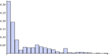
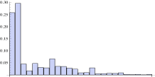
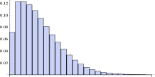
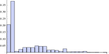
Figure 1: Initial (on the left) and long-time equilibrium (on the right) distributions for the model in Example $3.1.1$. Notice that the histograms are scaled differently on different pictures.

  initial asymptotic initial asymptotic initial asymptotic $x_{1}$ $0.321732$ $0.071378$ $0.257386$ $0.071371$ $0.205908$ $0.071368$ $x_{2}$ $0.193243$ $0.122656$ $0.296198$ $0.122646$ $0.378561$ $0.122643$ $x_{3}$ $0.083916$ $0.122567$ $0.045308$ $0.122560$ $0.009230$ $0.122558$ $x_{4}$ $0.021416$ $0.117529$ $0.017133$ $0.117524$ $0.024517$ $0.117523$ $x_{5}$ $0.039693$ $0.107903$ $0.047480$ $0.107901$ $0.037439$ $0.107901$ $x_{6}$ $0.034564$ $0.094594$ $0.031059$ $0.094595$ $0.037462$ $0.094595$ $x_{7}$ $0.036266$ $0.080894$ $0.029012$ $0.080896$ $0.036663$ $0.080898$ $x_{8}$ $0.052777$ $0.067416$ $0.066430$ $0.067421$ $0.049530$ $0.067423$ $x_{9}$ $0.041546$ $0.054706$ $0.035146$ $0.054711$ $0.045536$ $0.054714$ $x_{10}$ $0.034848$ $0.043194$ $0.034848$ $0.043200$ $0.045453$ $0.043203$ $x_{11}$ $0.028657$ $0.033173$ $0.028657$ $0.033179$ $0.018357$ $0.033180$ $x_{12}$ $0.023959$ $0.024781$ $0.023959$ $0.024786$ $0.019167$ $0.024787$ $x_{13}$ $0.010926$ $0.018017$ $0.008741$ $0.018022$ $0.016124$ $0.018023$ $x_{14}$ $0.005316$ $0.012767$ $0.009536$ $0.012771$ $0.008663$ $0.012771$ $x_{15}$ $0.031142$ $0.008837$ $0.029107$ $0.008839$ $0.027389$ $0.008839$ $x_{16}$ $0.005713$ $0.005992$ $0.004570$ $0.005993$ $0.004570$ $0.005993$ $x_{17}$ $0.003274$ $0.004126$ $0.005494$ $0.004127$ $0.005494$ $0.004126$ $x_{18}$ $0.007481$ $0.002892$ $0.006404$ $0.002892$ $0.006404$ $0.002891$ $x_{19}$ $0.007814$ $0.002064$ $0.006251$ $0.002062$ $0.006251$ $0.002062$ $x_{20}$ $0.005718$ $0.001494$ $0.008767$ $0.001493$ $0.008767$ $0.001492$ $x_{21}$ $0.004265$ $0.001091$ $0.002223$ $0.001090$ $0.002223$ $0.001089$ $x_{22}$ $0.000415$ $0.000797$ $0.001502$ $0.000795$ $0.001502$ $0.000795$ $x_{23}$ $0.002820$ $0.000576$ $0.002289$ $0.000574$ $0.002289$ $0.000574$ $x_{24}$ $0.000483$ $0.000406$ $0.000483$ $0.000405$ $0.000483$ $0.000405$ $x_{25}$ $0.002017$ $0.000147$ $0.002017$ $0.000147$ $0.002017$ $0.000147$  Table 3.1.1 The initial and the asymptotic components of the three solutions in Figure $1$.

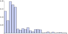
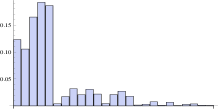
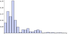
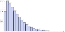
Figure 2: Initial (on the left) and long-time equilibrium (on the right) distributions for the model in Example $3.1.2$. Notice that the histograms are scaled differently on different pictures.

  initial asymptotic initial asymptotic initial asymptotic $x_{1}$ $0.136714$ $0.099140$ $0.123043$ $0.099140$ $0.080728$ $0.099140$ $x_{2}$ $0.078092$ $0.154143$ $0.105435$ $0.154143$ $0.171057$ $0.154143$ $x_{3}$ $0.196837$ $0.138916$ $0.164849$ $0.138916$ $0.130391$ $0.138916$ $x_{4}$ $0.176736$ $0.121397$ $0.192032$ $0.121397$ $0.254674$ $0.121397$ $x_{5}$ $0.161621$ $0.103429$ $0.185978$ $0.103429$ $0.101834$ $0.103429$ $x_{6}$ $0.025700$ $0.086143$ $0.003927$ $0.086143$ $0.048330$ $0.086143$ $x_{7}$ $0.018566$ $0.070253$ $0.017495$ $0.070253$ $0.006526$ $0.070253$ $x_{8}$ $0.028615$ $0.056173$ $0.032066$ $0.056173$ $0.027059$ $0.056173$ $x_{9}$ $0.022840$ $0.044083$ $0.020896$ $0.044083$ $0.025315$ $0.044083$ $x_{10}$ $0.034279$ $0.033987$ $0.030850$ $0.033987$ $0.036897$ $0.033987$ $x_{11}$ $0.015286$ $0.025764$ $0.022142$ $0.025764$ $0.011226$ $0.025764$ $x_{12}$ $0.008382$ $0.019219$ $0.004459$ $0.019219$ $0.009789$ $0.019218$ $x_{13}$ $0.022512$ $0.014118$ $0.021153$ $0.014118$ $0.021096$ $0.014118$ $x_{14}$ $0.023277$ $0.010220$ $0.027482$ $0.010220$ $0.026877$ $0.010220$ $x_{15}$ $0.020542$ $0.007294$ $0.018192$ $0.007294$ $0.018198$ $0.007294$ $x_{16}$ $0.001924$ $0.005136$ $0.001558$ $0.005136$ $0.001731$ $0.005136$ $x_{17}$ $0.002448$ $0.003570$ $0.003179$ $0.003570$ $0.002833$ $0.003570$ $x_{18}$ $0.008008$ $0.002450$ $0.007642$ $0.002450$ $0.007034$ $0.002450$ $x_{19}$ $0.001222$ $0.001660$ $0.001099$ $0.001660$ $0.002785$ $0.001660$ $x_{20}$ $0.006399$ $0.001112$ $0.006643$ $0.001112$ $0.005056$ $0.001112$ $x_{21}$ $0.000938$ $0.000736$ $0.000734$ $0.000736$ $0.001670$ $0.000736$ $x_{22}$ $0.002667$ $0.000481$ $0.002830$ $0.000481$ $0.002889$ $0.000481$ $x_{23}$ $0.003895$ $0.000311$ $0.003813$ $0.000311$ $0.003503$ $0.000311$ $x_{24}$ $0.001475$ $0.000199$ $0.001475$ $0.000199$ $0.001475$ $0.000199$ $x_{25}$ $0.001025$ $0.000069$ $0.001025$ $0.000069$ $0.001025$ $0.000069$  Table 3.1.2 The initial and the asymptotic components of the three solutions in Figure $2$.

Indeed, selecting, for a fixed $\mu\in[r_{1},r_{n}]$, various initial conditions $x_{0}\in\Sigma_{n-1}$ for which $\sum_{i=1}^{n}r_{i}x_{0i}=\mu$ hold true, we obtained results of the kind illustrated in the Figures $1$ and $2$.

Example $3.1.1$. Take $n=25$, the average incomes quadratically growing: $r_{j}=10\cdot j^{2}$ for $j=1,...,25$ and let the vector with tax rates components $\tau_{j}$ with $j=1,...,25$ be given by (0, 0.05, 0.1, 0.15, 0.2, 0.225, 0.25, 0.275, 0.3, 0.325, 0.35, 0.375, 0.4, 0.425, 0.45, 0.45, 0.45, 0.45, 0.45, 0.45, 0.45, 0.45, 0.45, 0.45, 0.45). E.g., the three solutions evolving from the initial distributions on the left in Figure $1$ tend in the future to the corresponding distributions on the right, which essentially coincide. The numerical values of the initial and the asymptotic components of the three solutions are given in the Table $3.1.1$. The constant value of the global wealth along the three solutions is $\mu=483$.

Example $3.1.2$. Take $n=25$, the average incomes linearly growing: $r_{j}=10\cdot j$ for $j=1,...,25$ and take the tax rate $\tau_{j}=\tau_{min}+(\tau_{max}-\tau_{min})\sqrt{(j-1)/24}$, where $\tau_{min}=0$ and $\tau_{max}=40/100$, for $j=1,...,25$. E.g., the three solutions evolving from the initial distributions on the left in Figure $1$ tend in the future to the corresponding distributions on the right, which essentially coincide. The numerical values of the initial and the asymptotic components of the three solutions are given in the Table $3.1.2$. The constant value of the global wealth along the three solutions is $\mu=52.52$.

3.2 Dependence of the asymptotic stationary distribution on the total wealth $\mu$

For fixed $n$ and fixed $r_{k}$ and $\tau_{k}$ we considered a list of different initial distributions corresponding to different values of the global wealth. We focused on long-time numerical solutions evolving from these distributions. Then, we fixed other values of $n$, of $r_{k}$ and $\tau_{k}$ and repeated the test.

We drew the conclusion that for a fixed model, the outline of the asymptotic stationary distribution depends on the conserved quantity $\mu$, which is related to the initial condition. In other words, we may say that there is a one-parameter family of asymptotic stationary distributions.

In this connection, we also want to emphasize a point, which will become clearer in the Subsection $3.4$. Other elements which, together with the value of global wealth $\mu$, have a decisive effect on the shape of the asymptotic distributions are the fact that in the framework described in this paper (only) a finite number of income classes are scheduled and the fact that, by (6), the number of individuals remains constant too.

3.3 Dependence of the asymptotic stationary distribution on the difference between the maximum and the minimum tax rate

Next we compare one with another different models.

In particular, for a fixed choice of $n$ and $r_{k}$ and for fixed total wealth $\mu$, we put to test different tax rates $\tau_{k}$. When doing that, it can be observed that the outline of the asymptotic stationary distribution depends on the difference between the maximum and the minimum tax rate, i.e. the rates respectively applied to the highest and to the lowest income classes. Specifically, to an increase of the difference between the maximum and the minimum tax rates $\tau_{max}$ and $\tau_{min}$, a growth of the middle classes at the asymptotic equilibrium corresponds, to the detriment of the poorest and the richest classes (see also [4]). For an illustrative purpose, we just report here the findings relative to one specific case.

Example $3.3.1$. Take $n=25$, the average incomes linearly growing: $r_{j}=10\cdot j$ for $j=1,...,25$ and take the tax rate $\tau_{j}=\tau_{min}+(\tau_{max}-\tau_{min})\sqrt{(j-1)/24}$. The Table $3.3.1$ reports the components of the asymptotic distributions corresponding to a same initial distribution for the three models in which the minimum and the maximum tax rate respectively are:

$$\begin{array}[]{lll}\hbox{case i)}:&\tau_{min}=20\%\,,&\tau_{max}=40\%\,,\\ \hbox{case ii)}:&\tau_{min}=10\%\,,&\tau_{max}=50\%\,,\\ \hbox{case iii)}:&\tau_{min}=0\%\,,&\tau_{max}=60\%\,.\end{array}$$

In the three cases the value of the total wealth is $\mu=50.43$.

Looking at the Table $3.3.1$, it is immediate noticing that the individual density in the first two classes, as well as in the last fourteen ones is smaller when the difference $\tau_{max}-\tau_{min}$ is larger. The reverse property does not hold true component-by-component for the middle classes. However, for them a collective property occurs: indeed, the total density of the of classes from the third to the $11$-th one is larger for larger $\tau_{max}-\tau_{min}$.

  case i) : 20%-40% case ii) : 10%-50% case iii) : 0%-60% $x_{1}$ $0.13261$ $0.11637,$ $0.09613$ $x_{2}$ $0.16666$ $0.16058$ $0.15558$ $x_{3}$ $0.13938$ $0.13983$ $0.14399$ $x_{4}$ $0.11544$ $0.11975$ $0.12761$ $x_{5}$ $0.09470$ $0.10079$ $0.10913$ $x_{6}$ $0.07694$ $0.08333$ $0.09041$ $x_{7}$ $0.06191$ $0.06765$ $0.07271$ $x_{8}$ $0.04935$ $0.05391$ $0.05686$ $x_{9}$ $0.03896$ $0.04216$ $0.04329$ $x_{10}$ $0.03048$ $0.03234$ $0.03212$ $x_{11}$ $0.02362$ $0.02434$ $0.02325$ $x_{12}$ $0.01814$ $0.01797$ $0.01643$ $x_{13}$ $0.01378$ $0.01301$ $0.01134$ $x_{14}$ $0.01041$ $0.00924$ $0.00766$ $x_{15}$ $0.00778$ $0.00643$ $0.00506$ $x_{16}$ $0.00576$ $0.00439$ $0.00327$ $x_{17}$ $0.00423$ $0.00294$ $0.00207$ $x_{18}$ $0.00308$ $0.00192$ $0.00128$ $x_{19}$ $0.00222$ $0.00124$ $0.00078$ $x_{20}$ $0.00158$ $0.00078$ $0.00046$ $x_{21}$ $0.00112$ $0.00048$ $0.00027$ $x_{22}$ $0.00079$ $0.00029$ $0.00015$ $x_{23}$ $0.00055$ $0.00017$ $0.00009$ $x_{24}$ $0.00038$ $0.00010$ $0.00005$ $x_{25}$ $0.00015$ $0.00003$ $0.00001$  Table 3.3.1 The components of the three asymptotic equilibria corresponding to three different taxation systems as described in the Example $3.3.1$.

3.4 Power-law distribution tails and dependence of the Pareto index on the total wealth $\mu$

Aiming at a deeper analysis of the properties of the asymptotic stationary distributions, we restricted attention on initial conditions, i.e. on initial distributions of the population, having the majority of individuals concentrated in lower income classes. To be concrete, we prescribed e.g. that a high percentage of individuals (in the example below, for example, $90\%$) belongs to the first five classes, another smaller percentage belongs to the second five classes, and so on. Such a restriction is motivated and justified by the fact that similar situations typically occur in real world societies. Using words of [14], we observe that non stationary initial distribution of individuals could be found “after a change in policy, e.g. after a change in the income tax schedule, or during a demographic transition, as many modern industrialized countries experience it right now”. We also point out in this connection that, since in our models the number of individuals does not change in time and only a finite number $n$ of income classes is considered, if a tail is expected in the asymptotic distribution, the global wealth cannot be too high. And this is obviously related to the mentioned realistic restriction.

The histograms of the asymptotic distributions seem to exhibit a power-law behavior of the distribution tails. Before showing that this behavior actually occurs and to see how to calculate the Pareto index [17], we make here a short digression on the relation between the discrete distribution of components $x_{i}$ and the continuous income distribution $f(w)$. We skip the variable $t$ since we have in mind here the asymptotic stationary distribution.

Consider an income interval $(w_{0},w_{0}+\Delta w)$, so small that the stationary distribution function $f(w)$ varies slowly in this interval, and yet such as to contain several discrete income classes $r(i)$, $r(i+1)$, …, $r(i+\Delta i)$. The income classes are chosen in such a way that $w_{0}=r(i)$ and $w_{0}+\Delta w=r(i+\Delta i)$. (Notice that $i$ is an integer variable and we usually denote the $i$-th income class with $r_{i}$; however, here we consider $r$ as a function of $i$, for reasons which will immediately be clear).

The population of the classes $i,...,i+\Delta i$ will also vary slowly, and we can write the total population in this interval as

$$f(w_{0})\,\Delta w=x_{i}\,\Delta i\,.$$

From this we see that the distribution function at $w_{0}$ is

$$f(w_{0})=x_{i}\,\frac{\Delta i}{\Delta w}\,.$$

But $\Delta w=r(i+\Delta i)-r(i)\simeq r^{\prime}(i)\,\Delta i$, so we obtain

$$f(w_{0})\simeq\frac{x_{i}}{r^{\prime}(i)}\,.$$

Generalizing to any $w$ such that $w=r(i)$, we have

$$f(w)\simeq\frac{x_{i}}{r^{\prime}(i)_{|_{i=r^{-1}(w)}}}\,.$$

For instance, if the classes are chosen so that the income increases quadratically, namely

$$r(i)=ci^{2}$$

for some constant $c>0$, then the distribution function with components $x_{i}$ corresponding to the equilibrium solution of our evolution equations is, at each point $w=r(i)$,

$$f(w)\simeq\frac{x_{i}}{2\sqrt{cw}}\,.$$

The power-law behavior $f(w)={C}{w^{-\alpha}}$ is equivalently expressed by the equation of a straight line: $\ln f(w)=\ln C-\alpha\ln w$. Therefore, to check whether the distribution tail exhibits it and to compute the Pareto index, we must have a linear fit of the log-log plot in the variables $w$ and $f$. What is known as Pareto index is the number $\beta=\alpha-1$.

According to a quantity of empirical data relative to several countries with capitalistic economies, Pareto assessed the index $\beta$ to be approximately equal to $1.5$. More generally, $\beta$ was observed to take values between $1$ and $2$.

As for the models described in this paper, the power-law property has been checked in several cases, namely for several different choices of the parameters. In particular, the following example illustrates the power-law behavior of the asymptotic distribution tail for a specific model.

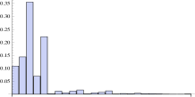
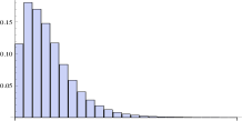
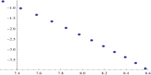
Figure 3: The left and the central panel respectively illustrate an initial and its corresponding long-time equilibrium distribution for the model in Example $3.4.1$. In the right panel the log-log plot is reported. Similarly as in previous figures, the histograms are scaled differently on the left and the central panel.

Example $3.4.1$. Take $n=25$, the average incomes quadratically growing: $r_{j}=10\cdot j^{2}$ for $j=1,...,25$ and let the vector with tax rates components $\tau_{j}$ with $j=1,...,25$ be given by (0, 0.1, 0.2, 0.3, 0.4, 0.41, 0.42, 0.43, 0.44, 0.45, 0.45, 0.45, 0.45, 0.45, 0.45, 0.45, 0.45, 0.45, 0.45, 0.45, 0.45, 0.45, 0.45, 0.45, 0.45). The histograms on the left panel in Figure $3$ correspond to an initial distribution, whose asymptotic distribution is in the central panel. In the panel on the right the log-log plot is illustrated, consisting of the sequence of points $(\ln(r_{i}),\ln(x_{i}/2\sqrt{(10r_{i})}))$. The value of the total wealth is in this case $\mu=271$ and the Pareto index is $1.7$.

A further property, we want to emphasize is the seemingly monotone dependence of the Pareto index, and equivalently of the exponent $\alpha$, on the value $\mu$ of the total wealth. We tested this property on several different models. Here we illustrate it with reference to the model described in the Example $3.4.1$: we next list a discrete number of values $\mu$ of the total wealth together with the values $\alpha$ of the corresponding power-law exponents. The values in the list show that $\alpha$ (and hence, also the Pareto index) decreases as $\mu$ increases.

$\mu$	$\alpha$
$231.5$	$2.81293$
$258.0$	$2.76824$
$284.5$	$2.70829$
$309.0$	$2.63832$
$337.5$	$2.56059$
$380.5$	$2.39970$
$400.0$	$2.32653$
$428.5$	$2.23525$
$463.0$	$2.11647$
$497.0$	$1.96068$

3.5 The Lorenz curve and the Gini coefficient

The Gini coefficient is commonly (and not only) used as a measure of inequality of income or wealth. It can range from the value $0$, expressing complete equality, to the value $1$, expressing maximal inequality. It is obtained based on the Lorenz curve, which plots the cumulative percentage of the total income of a population (on the $y$ axis) earned by the bottom percentage of individuals (on the $x$ axis). In comparison with it, the line at $45$ degrees represents a perfect equality of incomes. The Gini coefficient is defined as the ratio of the area between the Lorenz curve and the line of perfect equality and the total area under the line of perfect equality.

Example $3.5.1$. Consider the model described in the Example $3.4.1$. In Figure $4$ the line of perfect equality and the Lorenz curve relative to the asymptotic income distribution with total wealth $\mu=202$ are shown.

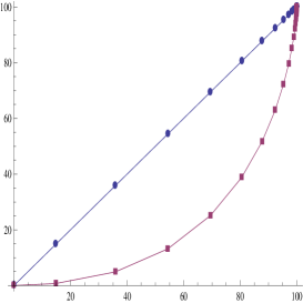
Figure 4: The line of perfect equality and the Lorenz curve relative to the asymptotic income distribution with total wealth $\mu=202$.

Here are the values of the Gini coefficient $i_{G}$, corresponding to the asymptotic distributions with a discrete choice of values of the total wealth $\mu$. To estimate them, we calculated the area under the Lorenz curve as a sum of areas of trapezia. Our purpose here is simply to show that the outputs of the family of models discussed exhibit possible agreement with real world data. Gini indices as those reported below correspond for example to empirical data relative to the income in Brazil [8].

$\mu$	$i_{G}$
$202$	$0.588604$
$226$	$0.592764$
$244$	$0.596331$
$259$	$0.598582$
$279$	$0.601564$

4 Conclusions

A general framework is here discussed, within which the taxation and redistribution process in a closed society can be described and the evolution of the income distribution analyzed. The framework is expressed by a system of nonlinear ordinary differential equations, in which a number of parameters appear. Fixing the parameter values amounts to formulating a specific model. Relaxation to a stationary distribution exhibiting a Pareto type tail has been found in several cases. Although rough and naive, the proposed models allow a possible explanation of the shape of income distributions commonly observed in real world economies. In a further perspective, the framework is suitable for the construction of explorative models. For example, it could be employed towards understanding which taxation system would be more desirable.

Future investigations should try to take one step further incorporating in the models, beside money exchanges, also assets and material possessions. Also, it would be of interest somehow keeping into account tax evasion phenomena and checking their effects on the income and wealth distributions.

References

- [1] W.B. Arthur, Complexity and the Economy, Science, 284, 107–109 (1999).
- [2] E. Ben-Naim, P.L. Krapivsky, F. Vazquez and S. Redner, Unity and discord in opinion dynamics, Physica A, 330, 99–106 (2003).
- [3] N. Bellomo, Modeling Complex Living Systems. A Kinetic Theory and Stochastic Game Approach, Birkäuser (2008).
- [4] M.L. Bertotti, Modelling taxation and redistribution: A discrete active particle kinetic approach, Appl. Math. Comput., 217, 752–762 (2010).
- [5] M.L. Bertotti, M. Delitala, On a discrete kinetic approach for modelling persuaders influence in opinion formation processes Math. Comput. Modelling, 48, 1107–1121 (2008).
- [6] M.L. Bertotti, M. Delitala, Cluster formation in opinion dynamics: a qualitative analysis, Z. Angew. Math. Phys., 61, 583–602 (2010).
- [7] A.S. Chakrabarti, B.K. Chakrabarti, Microeconomics of the ideal gas like market models, Physica A, 388, 4151–4158 (2009).
- [8] F. Chami Figueira, N.J. Moura Jr., M.B. Ribeiro, The Gompertz-Pareto income distribution, Physica A, 390, 689–698 (2011).
- [9] A. Chatterjee, B.K. Chakrabarti, Kinetic exchange models for income and wealth distributions, Eur. Phys. J. B, 60, 135–149 (2007).
- [10] F. Clementi, M. Gallegati, Power law tails in the Italian personal income distribution, Physica A, 350, 427–438 (2005).
- [11] B. Düring, D. Matthes, G. Toscani Kinetic equations modelling wealth redistribution: a comparison of approaches, Phys. Rev. E (3), 78, 05613 (2008).
- [12] B. Düring, D. Matthes, G. Toscani A Boltzmann-type approach to the formation of wealth distribution curves, Riv. Mat. Univ. Parma (8), 1, 199–261 (2009).
- [13] A. Grabowski and R.A. Kosinski, Ising-based model of opinion formation in a complex network of interpersonal interactions, Physica A, 361, 651–664 (2006).
- [14] B. Heer, A. Maussner, Dynamic General Equilibrium Modeling, Springer (2009).
- [15] R.N. Mantegna, H.E. Stanley, An Introduction to Econophysics, Cambridge University Press (2000).
- [16] M.E.J. Newman, Power laws, Pareto distributions and Zipf’s law, Contemp. Phys., 46, 323–351 (2005).
- [17] V. Pareto, Course d’Economie Politique, Lausanne (1896-7).
- [18] M. Patriarca, E. Heinsalu, A. Chakraborti, Basic kinetic wealth-exchange models: common features and open problems, Eur. Phys. J. B, 73, 145–153 (2010).
- [19] S. Sinha, B.K. Chakrabarti, Towards a physics of economics, Physics News (Bullettin of the Indian Physical Association), 39, 33–46 (2009).
- [20] V.M. Yakovenko, J. Barklry Rosser Jr., Colloquium: Statistical mechanics of money, wealth, and income, Rev. Mod. Phys., 81, 1703–1725 (2009).
- [21] G. Weisbuch, G. Deffuant and F. Amblard, Persuasion Dynamics, Physica A, 353, 555–575 (2005).
- [22] Banca d’Italia, Supplementi al Bollettino Statistico, I bilanci delle famiglie italiane nell’anno , Anno XVIII - 28 gennaio 2008, 7, www.bancaditalia.it.
- [23] Banca d’Italia, Supplementi al Bollettino Statistico, I bilanci delle famiglie italiane nell’anno , Anno XX - 10 febbraio 2010, 8, www.bancaditalia.it.
- [24] ISTAT, Condizioni di vita e distribuzione del reddito in Italia. Anno , 29 dicembre 2009, www.istat.it.