Approximate Counting via Correlation Decay in Spin Systems

Abstract

We give the first deterministic fully polynomial-time approximation scheme (FPTAS) for computing the partition function of a two-state spin system on an arbitrary graph, when the parameters of the system satisfy the uniqueness condition on infinite regular trees. This condition is of physical significance and is believed to be the right boundary between approximable and inapproximable.

The FPTAS is based on the correlation decay technique introduced by Bandyopadhyay and Gamarnik [SODA 06] and Weitz [STOC 06]. The classic correlation decay is defined with respect to graph distance. Although this definition has natural physical meanings, it does not directly support an FPTAS for systems on arbitrary graphs, because for graphs with unbounded degrees, the local computation that provides a desirable precision by correlation decay may take super-polynomial time. We introduce a notion of computationally efficient correlation decay, in which the correlation decay is measured in a refined metric instead of graph distance. We use a potential method to analyze the amortized behavior of this correlation decay and establish a correlation decay that guarantees an inverse-polynomial precision by polynomial-time local computation. This gives us an FPTAS for spin systems on arbitrary graphs. This new notion of correlation decay properly reflects the algorithmic aspect of the spin systems, and may be used for designing FPTAS for other counting problems.

1 Introduction

Spin systems are well studied in Statistical Physics. We focus on two-state spin systems. An instance of a spin system is a graph $G=(V,E)$. A configuration $\sigma:V\rightarrow\{0,1\}$ assigns every vertex one of the two states. We shall refer the two states as blue and green. The contributions of local interactions between adjacent vertices are quantified by a matrix

$$A=\begin{bmatrix}A_{0,0}&A_{0,1}\\ A_{1,0}&A_{1,1}\end{bmatrix}=\begin{bmatrix}\beta&1\\ 1&\gamma\end{bmatrix},$$

where $\beta,\gamma\geq 0$. The weight of an assignment is the production of contributions of all local interactions and the partition function $Z_{A}(G)$ of a system is the summation of the weights over all possible assignments. Formally,

$$Z_{A}(G)=\sum_{\sigma\in 2^{V}}\prod_{(u,v)\in E}A_{\sigma(u),\sigma(v)}.$$

Although originated from Statistical Physics, the spin system is also accepted in Computer Science as a framework for counting problems. Considering the two very well studied frameworks, the weighted Constraint Satisfaction Problems (#CSP) [14, 7, 26, 6, 12, 19, 11] and Graph Homomorphisms [17, 8, 28, 36, 10, 9], the two-state spin systems can be viewed as the most basic setting in these frameworks: A Boolean #CSP problem with one symmetric binary relation; or Graph Homomorphisms to graph with two vertices. Many natural combinatorial problems can be formulated as two-state spin systems. For example, with $\beta=0$ and $\gamma=1$, $Z_{A}(G)$ is the number of independent sets (or vertex covers) of the graph $G$.

Given a matrix $A$, it is a computational problem to compute $Z_{A}(G)$ where graph $G$ is given as input. We want to characterize the computational complexity of computing $Z_{A}(G)$ in terms of $\beta$ and $\gamma$. For exact computation of $Z_{A}(G)$, polynomial time algorithms are known only for the very restricted settings that $\beta\gamma=1$ or $(\beta,\gamma)=(0,0)$, and for all other settings the problem is proved to be #P-Hard [8]. We consider the approximation of $Z_{A}(G)$, with the fully polynomial-time approximation schemes (FPTAS) and its randomized relaxation the fully polynomial-time randomized approximation schemes (FPRAS).

In a seminal paper [48], Jerrum and Sinclair gave an FPRAS when $\beta=\gamma>1$, which was further extended to the entire region $\beta\gamma>1$ [41]. For $0\leq\beta,\gamma\leq 1$ except that $(\beta,\gamma)=(0,0)$ or $(1,1)$, Goldberg, Jerrum and Paterson prove that the problem do not admit an FPRAS unless NP$=$RP [41]. For the other values of the parameters, namely, $0\leq\beta<1<\gamma<\frac{1}{\beta}$ or symmetrically $0\leq\gamma<1<\beta<\frac{1}{\gamma}$, the approximability of $Z_{A}(G)$ is not very well understood. It was shown in [41] that by coupling a simple heat-bath random walk, there exists an additional region of $\beta$ and $\gamma$ which admit some FPRAS. The true characterization of approximability is still left open.

Within this unknown region, there lies a critical curve with physical significance, called the uniqueness threshold. The phase transition of Gibbs measure occurs at this threshold curve. Such statistical physics phase transitions are believed to coincide with the transitions of computational complexity. However, there are only very few examples where the connection is rigorously proved. One example is the hardcore (counting independent set) model. It was conjectured in [56] by Mossel, Weitz and Wormald, and settled in a line of works by Dyer, Frieze and Jerrum [23], Weitz [61], Sly [58], and very recently Galanis, Ge, Štefankovič, Vigoda and Yang [31] that in the hardcore model the uniqueness threshold essentially characterizes the approximability of the partition function. It will be very interesting to observe the similar transition in spin systems.

1.1 Main results

We extend the approximable region (in terms of $\beta$ and $\gamma$) of $Z_{A}(G)$ to the uniqueness threshold in two-state spin systems, which is believed to be the right boundary between approximable and inapproximable. Specifically, we formulate a criterion for $\beta$ and $\gamma$ such that there is a unique Gibbs measure on all infinite regular trees, and prove that there is an FPTAS for computing $Z_{A}(G)$ when this uniqueness condition is satisfied. This improves the approximable boundary (dashed lines in Figure 1) provided by the heat-bath random walk in [41]. Moreover, the algorithm is deterministic.

The FPTAS is based on the correlation decay technique first used in [61, 1] for approximate counting. We elaborate a bit on the ideas. A spin system induces a natural probability distribution over all configurations called the Gibbs measure where the probability of a configuration is proportional to its weight. Due to a standard self-reduction procedure, computing $Z_{A}(G)$ is reduced to computing the marginal distribution of the state of one vertex, which is made plausible by Weitz in [61] with the self-avoiding walk (SAW) tree construction. For efficiency of computation, the marginal distribution of a vertex is estimated using only a local neighborhood around the vertex. To justify the precision of the estimation, we show that far-away vertices have little influence on the marginal distribution. This is done by analyzing the rate with which the correlation between two vertices decays as they are far away from each other.

The correlation decay by itself is a phenomenon of physical significance. One of our main discoveries is that two-state spin systems on any graphs have exponential correlation decay when the above uniqueness condition is satisfied.

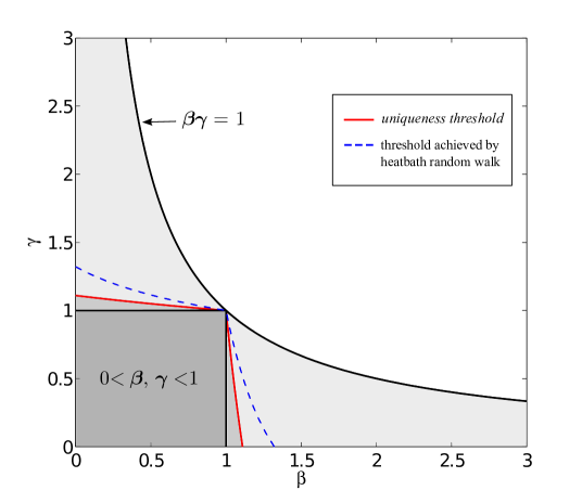
Figure 1: Our FPTAS works for the region between the critical curve of the uniqueness threshold and the curve $\beta\gamma=1$. The heat-bath random walk in [41] works for the region between the dashed line and $\beta\gamma=1$.

1.2 Technical contributions

The technique of using correlation decay to design FPTAS for partition functions is developed in the hardcore model. We introduce several new ideas to adapt the challenges arising from spin systems. We believe these challenges are typical in counting problems, and the new ideas will make the correlation decay technique more applicable for approximate counting.

1. The correlation decay technique used in [61] relies on a monotonicity property specific to the hardcore model. Correlation decays in graphs are reduced via this monotonicity to the decays in infinite regular trees, while the later have solvable phase transition thresholds. It was already observed in [61] that such monotonicity may not generally hold for other models. Indeed, it does not hold for spin systems. We develop a more general method which does not rely on monotonicity: We directly compute the correlation decay in arbitrary trees (and as a result in arbitrary graphs via the SAW tree reduction), and use the potential method to analyze the amortized behavior of correlation decay.

2. To have an FPTAS, the marginal distribution of a single vertex should be approximable up to certain precision from a local neighborhood of polynomial size. The classic correlation decay is measured with respect to graph distance. The local neighborhoods in this sense are balls in the graph metric. A SAW tree enumerates all paths originating from a vertex. For graphs of unbounded degrees, the SAW tree transformation may have the balls offering desirable precisions explode to super-polynomial sizes.

   We introduce the notion of computationally efficient correlation decay. Correlation decay is now measured in a refined metric, which has the advantage that a desirable precision is achievable by a ball (in the new metric) of polynomial size even after the SAW tree transformation. We prove an exponential correlation decay in this new metric when the uniqueness is satisfied. As a result, we have an FPTAS for arbitrary graphs as long as the uniqueness condition holds.

1.3 Related works

The approximation for partition function has been extensively studied with both positive [48, 50, 39, 18, 29, 47, 60] and negative results [38, 5, 56, 37, 13, 33, 3, 32]. Some special problems in these framework are well studied combinatorial problems, e.g. counting independent sets [23, 29, 53] and graph coloring [54, 47, 45, 20, 22, 43, 21, 44, 46, 30, 55, 60, 4, 40]. Some dichotomies (or trichotomies) of complexity for approximate counting CSP were also obtained [27, 24, 31, 58]. Almost all known approximation counting algorithms are based on random sampling [51, 25], usually through the famous Markov Chain Monte Carlo (MCMC) method [16, 49]. There are very few deterministic approximation algorithms for any counting problems. Some notable examples include [1, 34, 2, 42, 59].

In a very recent work [57], Sinclair, Srivastava, and Thurley give an FPTAS using correlation decay for the two-state spin systems on bounded degree graphs. They allow the two-state spin systems to have an external field, and the uniqueness thresholds they used are defined with respect to specific maximum degrees.

2 Definitions and Statements of Results

A spin system is described by a graph $G=(V,E)$. A configuration of the system is one of the $2^{|V|}$ possible assignments $\sigma:V\rightarrow\{0,1\}$ of states to vertices. We also use two colors blue and green to denote these two states. Let $A=\begin{bmatrix}A_{0,0}&A_{0,1}\\ A_{1,0}&A_{1,1}\end{bmatrix}=\begin{bmatrix}\beta&1\\ 1&\gamma\end{bmatrix}$, where $\beta,\gamma\geq 0$. The Gibbs measure is a distribution over all configurations defined by

$$\mu(\sigma)=\frac{1}{Z_{A}(G)}\prod_{(u,v)\in E}A_{\sigma(u),\sigma(v)}.$$

The normalization factor $Z_{A}(G)=\sum_{\sigma\in 2^{V}}\prod_{(u,v)\in E}A_{\sigma(u),\sigma(v)}$ is called the partition function.

From this distribution, we can define the marginal probability $p_{v}$ of $v$ to be colored blue. Let $\sigma_{\Lambda}$ be a configuration defined on vertices in $\Lambda\subset V$. We call vertices $v\in\Lambda$ fixed vertices, and $v\not\in\Lambda$ free vertices. We use $p_{v}^{\sigma_{\Lambda}}$ to denote the marginal probability of $v$ to be colored blue conditioned on the configuration of $\Lambda$ being fixed as $\sigma_{\Lambda}$.

Definition 1

A spin system on a family of graphs is said to have exponential correlation decay if for any graph $G=(V,E)$ in the family, any $v\in V,\Lambda\subset V$ and $\sigma_{\Lambda},\tau_{\Lambda}\in\{0,1\}^{\Lambda}$,

$$|p_{v}^{\sigma_{\Lambda}}-p_{v}^{\tau_{\Lambda}}|\leq\exp(-\Omega(\mathrm{dist}(v,\Delta))).$$

where $\Delta\subset\Lambda$ is the subset on which $\sigma_{\Lambda}$ and $\tau_{\Lambda}$ differ, and $\mathrm{dist}(v,\Delta)$ is the shortest distance from $v$ to any vertex in $\Delta$.

This definition is equivalent to the “strong spatial mixing” in [61] with an exponential rate. It is stronger than the standard notion of exponential correlation decay in Statistical Physics [15], where the decay is measured with respect to $\mathrm{dist}(v,\Lambda)$ instead of $\mathrm{dist}(v,\Delta)$.

The marginal probability $p_{v}^{\sigma_{\Lambda}}$ in a tree can be computed by the following recursion. Let $T$ be a tree rooted by $v$. We denote $R_{T}^{\sigma_{\Lambda}}$ as the ratio of the probabilities that root $v$ is blue and green, respectively, when imposing the condition $\sigma_{\Lambda}$. Formally, $R_{T}^{\sigma_{\Lambda}}=\frac{p_{v}^{\sigma_{\Lambda}}}{1-p_{v}^{\sigma_{\Lambda}}}$ (when $p_{v}^{\sigma_{\Lambda}}=1$, let $R_{v}^{\sigma_{\Lambda}}=\infty$ by convention). Suppose that the root of $T$ has $d$ children. Let $T_{i}$ be the subtree rooted by the $i$-th child of the root. The distributions on distinct subtrees are independent. A calculation then gives that

$$R_{T}^{\sigma_{\Lambda}}=\prod_{i=1}^{d}\frac{\beta R_{T_{i}}^{\sigma_{\Lambda}}+1}{R_{T_{i}}^{\sigma_{\Lambda}}+\gamma}.$$ (1)

It is of physical significance to study the Gibbs measures on infinite $(d+1)$-regular trees $\widehat{\mathbb{T}}^{d}$ [35]. In $\widehat{\mathbb{T}}^{d}$, the recursion is of a symmetric form $f(x)=\left(\frac{\beta x+1}{x+\gamma}\right)^{d}$. There may be more than one Gibbs measures on infinite graphs. We say that the system has the uniqueness if there is exact one Gibbs measure. Let $\hat{x}=f(\hat{x})$ be the fixed point of $f(x)$. It is known [52, 54] that the spin system on $\widehat{\mathbb{T}}^{d}$ undergoes a phase transition at $|f^{\prime}(\hat{x})|=1$ with uniqueness when $|f^{\prime}(\hat{x})|=\frac{d(1-\beta\gamma)(\beta\hat{x}+1)^{d-1}}{(\hat{x}+\gamma)^{d+1}}\leq 1$. This motivates the following definition

$$\Gamma(\beta) =\inf\left\{\gamma\geq 1\Bigm{|}\forall d\geq 1,\,\frac{d(1-\beta\gamma)(\beta\hat{x}+1)^{d-1}}{(\hat{x}+\gamma)^{d+1}}\leq 1\right\}.$$

For a fixed $0\leq\beta<1$, the $\Gamma(\beta)$ gives the boundary that all infinite regular trees $\widehat{\mathbb{T}}^{d}$ exhibit uniqueness when $\Gamma(\beta)\leq\gamma\leq\frac{1}{\beta}$. We call $\Gamma(\beta)$ the uniqueness threshold. Indeed, for any $d\geq 1$, there is a critical $\Gamma_{d}(\beta)$ such that $\widehat{\mathbb{T}}^{d}$ exhibits uniqueness when $\Gamma_{d}(\beta)<\gamma<\frac{1}{\beta}$. Furthermore, there is a finite crucial $D>1$ such that $\Gamma_{D}(\beta)=\Gamma(\beta)$. That is, $\widehat{\mathbb{T}}^{D}$ has the highest uniqueness threshold $\Gamma(\beta)$ among all $\widehat{\mathbb{T}}^{d}$.

We remark that for technical reasons, we treat $d$ as real numbers thus $\Gamma(\beta)$ is slightly greater than the one defined by integer $d$s. An integer version of $\Gamma(\beta)$ is given in Section 6, where a slightly improved and tight analysis is given for the specially case $\beta=0$.

Definition 2

A fully polynomial-time approximation scheme (FPTAS) for $Z_{A}(G)$ is an algorithm that given as input an instance $G$ and an $\epsilon>0$, outputs a number $Z$ in time $\mathrm{poly}(|G|,\frac{1}{\epsilon})$ such that $(1-\epsilon)Z_{A}(G)\leq Z\leq(1+\epsilon)Z_{A}(G)$.

In Definition 1, the correlation decay is measured in graph distance. In order to support an FPTAS for graphs with unbounded degrees, we need to define the following refined metric.

Definition 3

Let $T$ be a rooted tree and $M\geq 2$ be a constant. We define the $M$-based depth $L_{M}(v)$ of a vertex $v$ in $T$ recursively as follows: $L_{M}(v)=0$ if $v$ is the root of $T$; and for every child $u$ of $v$, if $v$ has $d\geq 1$ children, $L_{M}(u)=L_{M}(v)+\lceil\log_{M}(d+1)\rceil$.

If every vertex in $T$ has $d<M$ children, $L_{M}(v)$ is precisely the depth of $v$. If there are vertices having $d\geq M$ children, we actually replace every such vertex and its $d$ children with an $M$-ary tree of depth $\lceil\log_{M}(d+1)\rceil$, and $L_{M}(v)$ is the depth of $v$ in this new tree.

Definition 4

Let $T$ be a rooted tree and $M\geq 2$ be a constant. Let $B_{M}(L)=\{v\in T\mid L_{M}(v)\leq L\}$, called an $M$-based $L$-ball, be the set of vertices in $T$ whose $M$-based depths are no greater than $L$; and let $B_{M}^{*}(L)$, called an $M$-based $L$-closed-ball, be the set of vertices in $B_{M}(L)$ and all their children in $T$.

The main technical result of the paper is the following theorem which establishes an exponential correlation decay in the refined metric when the uniqueness condition holds.

Theorem 5 (Computationally Efficient Correlation Decay)

Let $0\leq\beta<1$, $\beta\gamma<1$, and $\gamma>\Gamma(\beta)$. There exists a sufficiently large constant $M$ which depends only on $\beta$ and $\gamma$, such that on an arbitrary tree $T$, for any two configurations $\sigma_{\Lambda}$ and $\tau_{\Lambda}$ which differ on $\Delta\subset\Lambda$, if $B_{M}^{*}(L)\cap\Delta=\emptyset$ then

$$|R_{T}^{\sigma_{\Lambda}}-R_{T}^{\tau_{\Lambda}}|\leq\exp(-\Omega(L)).$$

The name computationally efficient correlation decay is due to the fact that $|B_{M}(L)|\leq M^{L}$ in any tree, thus an exponential decay would imply a polynomial-size $B_{M}(L)$ giving an inverse-polynomial precision.

Theorem 5 has the following implications via Weitz’s self-avoiding tree construction [61].

Theorem 6

Let $0\leq\beta<1$, $\beta\gamma<1$ , $\gamma>\Gamma(\beta)$. It is of exponential correlation decay for the Gibbs measure on any graph.

Theorem 7

Let $0\leq\beta<1$, $\beta\gamma<1$ , $\gamma>\Gamma(\beta)$. There is an FPTAS for computing the partition function $Z_{A}(G)$ for arbitrary graph $G$.

By symmetry, in Theorem 5, 6, and 7, the roles of $\beta$ and $\gamma$ can be switched.

In the Section 3, we will show the FPTAS implied by Theorem 5, followed by a formal treatment of the uniqueness threshold in Section 4, and finally the formal proof of Theorem 5 in Section 5.

3 An FPTAS for the Partition Function

Assuming that Theorem 5 is true, we show that when $0\leq\beta<1$ and $\Gamma(\beta)<\gamma<\frac{1}{\beta}$, there is an FPTAS for the partition function $Z_{A}(G)$ for arbitrary graph $G$. The FPTAS is based on approximation of $R_{G,v}^{\sigma_{\Lambda}}=p_{v}^{\sigma_{\Lambda}}/(1-p_{v}^{\sigma_{\Lambda}})$, the ratio between the probabilities that $v$ is blue and green, respectively, when imposing the condition $\sigma_{\Lambda}$.

The self-avoiding walk tree is introduced by Weitz in [61] for calculating $R_{G,v}^{\sigma_{\Lambda}}$. Given a graph $G=(V,E)$, we fix an arbitrary order $<$ of vertices. Originating from any vertex $v\in V$, a self-avoiding walk tree, denoted $T_{\mathrm{SAW}}(G,v)$, is constructed as follows. Every vertex in $T_{\mathrm{SAW}}(G,v)$ corresponds to one of the walks $v_{1}\rightarrow v_{2}\rightarrow\cdots\rightarrow v_{k}$ in $G$ such that $v_{1}=v$, all edges are distinct and $v_{1},\ldots,v_{k-1}$ are distinct, i.e. the self-avoiding walks originating from $v$ and those appended with a vertex closing a cycle. The root of $T_{\mathrm{SAW}}(G,v)$ corresponds to the trivial walk $v$. The vertex $v_{1}$ parents $v_{2}$ in $T_{\mathrm{SAW}}(G,v)$, if and only if their respective walks $w_{1}$ and $w_{2}$ satisfy that $w_{2}=w_{1}\rightarrow u$ for some $u$. For a leaf of $T_{\mathrm{SAW}}(G,v)$ whose walk closes a cycle, supposed that the cycle is $u\rightarrow v_{1}\rightarrow\cdots v_{k}\rightarrow u$, fix the leaf to be blue if $v_{1}>v_{k}$ and green otherwise. When a configuration $\sigma_{\Lambda}$ is imposed on $\Lambda\subset V$ of the original graph $G$, for any vertex of $T_{\mathrm{SAW}}(G,v)$ whose corresponding walk ends at a $u\in\Lambda$, the color of the vertex is fixed to be $\sigma_{\Lambda}(u)$. We abuse the notation and denote the resulting configuration on $T_{\mathrm{SAW}}(G,v)$ by $\sigma_{\Lambda}$ as well.

This novel tree construction has the advantage that the probabilities are exactly the same in both the original spin system and the constructed tree.

Theorem 8 (Weitz [61])

Let $T=T_{\mathrm{SAW}}(G,v)$. It holds that $R^{\sigma_{\Lambda}}_{G,v}=R^{\sigma_{\Lambda}}_{T}$

Due to (1), in a tree $T$, the following recursion holds for $R_{T}^{\sigma_{\Lambda}}$:

$$R_{T}^{\sigma_{\Lambda}} =\prod_{i=1}^{d}\frac{\beta R_{T_{i}}^{\sigma_{\Lambda}}+1}{R_{T_{i}}^{\sigma_{\Lambda}}+\gamma}.$$

The base case is either when the current root $v\in\Lambda$, i.e. $v$’s color is fixed, in which case $R_{T}^{\sigma_{\Lambda}}=\infty$ or $R_{T}^{\sigma_{\Lambda}}=0$ (depending on whether $v$ is fixed to be blue or green), or when $v$ is free and has no children, in which case $R_{T}^{\sigma_{\Lambda}}=1$ (this is consistent with the recursion since the outcome of an empty product is 1 by convention).

For $\beta\gamma<1$, the recursion is monotonically decreasing with respect to every $R_{T_{i}}^{\sigma_{\Lambda}}$. An upper (lower) bound of $R_{T}^{\sigma_{\Lambda}}$ can be computed by replacing $R_{T_{i}}^{\sigma_{\Lambda}}$ in the recursion by their respective lower (upper) bounds. Algorithm 1 computes the lower or upper bound of $R_{T}^{\sigma_{\Lambda}}$ up to vertices in $M$-based $L$-closed ball $B_{M}^{*}(L)$. For the vertices outside $B_{M}^{*}(L)$, it uses the trivial bounds $0\leq R\leq\infty$.

$R(T_{v},\sigma_{\Lambda},L,d_{\mathrm{parent}},lb)$:

Input: Rooted tree $T_{v}$; configuration $\sigma_{\Lambda}$; $M$-based depth $L$; parent degree $d_{\mathrm{parent}}$; Boolean indicator $lb$ of lower bound.

Output: Lower (or upper) bound of $R_{T}^{\sigma_{\Lambda}}$ computed from vertices in $B_{M}^{*}(L)$.

begin

       Suppose root $v$ has $d$ children and let $T_{i}$ be the subtree rooted by the $i$-th child;

       if $v\in\Lambda$ then

             if $\sigma_{\Lambda}(v)=\mathtt{blue}$ then return $\infty$;

            ;

             else  return $0$;

            ;

            

      else if $L<0$ then

            if $lb=\mathtt{true}$ then return $0$;

            ;

             else  return $\infty$;

            ;

            

      else

             $L^{\prime}\longleftarrow L-\lceil\log_{M}(d_{\mathrm{parent}}+1)\rceil$;

             return $\prod_{i=1}^{d}\frac{\beta R(T_{i},\sigma_{\Lambda},L^{\prime},d,\neg lb)+1}{R(T_{i},\sigma_{\Lambda},L^{\prime},d,\neg lb)+\gamma}$;

            

      

Algorithm 1 Estimate $R_{T}^{\sigma_{\Lambda}}$ based on $B_{M}^{*}(L)$

Due to the monotonicity of the recursion, it holds that

$$R(T,\sigma_{\Lambda},L,0,\mathtt{true})\leq R_{T}^{\sigma_{\Lambda}}\leq R(T,\sigma_{\Lambda},L,0,\mathtt{false}).$$

Note that the naive lower bound $0$ (or the upper bound $\infty$) of $R$ for a vertex outside $B_{M}^{*}(L)$ can be achieved by fixing the vertex to be green (or blue). Denote by $\tau_{0}$ and $\tau_{1}$ the configurations achieving the lower and upper bounds respectively. It is easy to see that $\tau_{0}=\tau_{1}=\sigma_{\Lambda}$ in $B_{M}^{*}(L)$. Then due to Theorem 5, there is a constant $\alpha<1$ such that

$$\quad\,\,|R(T,\sigma_{\Lambda},L,0,\mathtt{false})-R(T,\sigma_{\Lambda},L,0,\mathtt{true})|$$

$$=|R_{T}^{\tau_{1}}-R_{T}^{\tau_{0}}|$$

$$=O(\alpha^{L}).$$

To compute $R_{G,v}^{\sigma_{\Lambda}}$ for an arbitrary graph $G$, we first construct the $B_{M}^{*}(L)$ of $T=T_{\mathrm{SAW}}(G,v)$, and run Algorithm 1. Due to Theorem 8, $R_{G,v}^{\sigma_{\Lambda}}=R_{T}^{\sigma_{\Lambda}}$, thus it returns $R_{0}$ and $R_{1}$ such that $R_{0}\leq R_{G,v}^{\sigma_{\Lambda}}\leq R_{1}$ and $R_{1}-R_{0}=O(\alpha^{L})$. Since $p_{v}^{\sigma_{\Lambda}}=R_{G,v}^{\sigma_{\Lambda}}/(1+R_{G,v}^{\sigma_{\Lambda}})$, we can output $p_{0}=\frac{R_{0}}{R_{0}+1}$ and $p_{1}=\frac{R_{1}}{R_{1}+1}$ so that $p_{0}\leq p_{v}^{\sigma_{\Lambda}}\leq p_{1}$ and $p_{1}-p_{0}=\frac{R_{1}}{R_{1}+1}-\frac{R_{0}}{R_{0}+1}\leq R_{1}-R_{0}=O(\alpha^{L})$.

The running time of this algorithm relies on the size of $B_{M}^{*}(L)$ in $T_{\mathrm{SAW}}(G,v)$. The maximum degree of $T_{\mathrm{SAW}}(G,v)$ is bounded by the maximum degree of $G$, which is trivially bounded by $n$, thus $|B_{M}^{*}(L)|\leq n|B_{M}(L)|\leq nM^{L}$. The running time of the algorithm is $O(|B_{M}^{*}(L)|)=O(nM^{L})$.

By setting $L=\log_{\alpha}\epsilon$, we can approximate $1-p_{v}^{\sigma_{\Lambda}}$ within absolute error $O(\epsilon)$ in time $O(n\cdot\mathrm{poly}(\frac{1}{\epsilon}))$. For $\beta<1<\gamma$, it holds that $0<R_{G,v}^{\sigma_{\Lambda}}<1$ for free $v$ thus $1-p_{v}^{\sigma_{\Lambda}}>\frac{1}{2}$, therefore the above procedure approximates $(1-p_{v}^{\sigma_{\Lambda}})$ within factor $(1\pm O(\epsilon))$. We have an FPTAS for $(1-p_{v}^{\sigma_{\Lambda}})$.

The partition function $Z_{A}(G)$ can be computed from $p_{v}^{\sigma_{\Lambda}}$ by the following standard routine. Let $v_{1},\ldots,v_{n}$ enumerate the vertices in $G$, and let $\sigma_{i},i=0,1,\ldots,n$, be the configurations fixing the first $i$ vertices $v_{1},\ldots,v_{i}$ to be green, where $\sigma_{0}$ means all vertices are free. The probability measure of $\sigma_{n}$ (all green) can be computed as

$$\mu(\sigma_{n}) =\prod_{i=1}^{n}\Pr[v_{i}\text{ is green }\mid v_{1},\ldots,v_{i-1}\text{ are green}]$$

$$=\prod_{i=1}^{n}(1-p_{v_{i}}^{\sigma_{i-1}}).$$

On the other hand, it is easy to see that $\mu(\sigma_{n})=\frac{\gamma^{|E|}}{Z_{A}(G)}$ by definition of $\mu$. Thus

$$Z_{A}(G) =\frac{\gamma^{|E|}}{\mu(\sigma_{n})}=\frac{\gamma^{|E|}}{\prod_{i=1}^{n}(1-p_{v_{i}}^{\sigma_{i-1}})}.$$

Notice that $\gamma^{|E|}>1$. Therefore, an FPTAS for $(1-p_{v}^{\sigma_{\Lambda}})$ implies an FPTAS for $Z_{A}(G)$.

4 The uniqueness threshold

In this section, we formally define the uniqueness threshold $\Gamma(\beta)$ and the critical $D$. We also prove several propositions regarding these quantities which are useful for the analysis of the correlation decay.

Definition 9

Let $0\leq\beta<1$ be a fixed parameter. Suppose that $1\leq\gamma<\frac{1}{\beta}$ and $d\geq 1$. Let $x(\gamma,d)$ be the positive solution of

$$x =\left(\frac{\beta x+1}{x+\gamma}\right)^{d}.$$ (2)

Define that $f(x)=\left(\frac{\beta x+1}{x+\gamma}\right)^{d}$. Then $x(\gamma,d)$ is the positive fixed point of $f(x)$. For $\gamma<\frac{1}{\beta}$, $f(x)=\left(\beta+\frac{1-\beta\gamma}{x+\gamma}\right)^{d}$ is continuous and strictly decreasing over $x\in[0,\infty)$, and it holds that $f(0)=\frac{1}{\gamma^{d}}>0$ and $f(1)=\left(\frac{1+\beta}{1+\gamma}\right)^{d}<\frac{1}{\gamma^{d}}\leq 1$, thus $f(x)$ has a unique fixed point over $x\in(0,1)$. Therefore, for $1\leq\gamma<\frac{1}{\beta}$ and $d\geq 1$, $x(\gamma,d)$ is well defined and $x(\gamma,d)\in(0,1)$.

Definition 10

Let

$$\Gamma(\beta) =\inf\left\{\gamma\geq 1\Bigm{|}\forall d\geq 1,\,\frac{d(1-\beta\gamma)(\beta x(\gamma,d)+1)^{d-1}}{(x(\gamma,d)+\gamma)^{d+1}}\leq 1\right\}.$$

We write $\Gamma=\Gamma(\beta)$ for short if no ambiguity is caused.

Note that $\Gamma$ can be equivalently defined as

$$\Gamma =\inf\left\{\gamma\geq 1\Bigm{|}\forall d\geq 1,\,\frac{d(1-\beta\gamma)x(\gamma,d)}{\left(\beta x(\gamma,d)+1\right)\left(x(\gamma,d)+\gamma\right)}\leq 1\right\},$$

because $x(\gamma,d)$ satisfies (2).

The following lemma states that for $0\leq\beta<1$, $\Gamma(\beta)$ is well-defined and nontrivial.

Lemma 11

For $0\leq\beta<1$, it holds that $1<\Gamma(\beta)<\frac{1}{\beta}$.

Proof: We first show that $\Gamma>1$. It is sufficient to show that if $\gamma\leq 1$ then there exists a $d$ such that $\frac{d(1-\beta\gamma)x}{(\beta x+1)(x+\gamma)}>1$, where $x$ satisfies that $x=\left(\frac{\beta x+1}{x+\gamma}\right)^{d}$.

By contradiction, suppose that $\gamma\leq 1$ and for all $d\geq 1$, $\frac{d(1-\beta\gamma)x}{(\beta x+1)(x+\gamma)}\leq 1$ where $x$ satisfies that $x=\left(\frac{\beta x+1}{x+\gamma}\right)^{d}$. Then,

$$1\geq\frac{d(1-\beta\gamma)x}{(\beta x+1)(x+\gamma)}=\frac{d(1-\beta\gamma)}{\beta x+\frac{\gamma}{x}+(1+\beta\gamma)}\geq\frac{d(1-\beta\gamma)}{\beta x+\frac{\gamma}{x}+2}.$$

Specifically, suppose that $d$ is sufficiently large so the followings hold

$$\beta^{d}\exp\left(\frac{d}{(1-\beta\gamma)d-3}\right) <\frac{d(1-\beta\gamma)-3}{\beta},\text{ and}$$

$$\exp\left(-\frac{\gamma d}{d(1-\beta\gamma)-3}\right) >\frac{\gamma}{d(1-\beta\gamma)-3}.$$

• $x\geq\gamma$. Then $\frac{\gamma}{x}\leq 1$. Thus,

  $$1\geq\frac{d(1-\beta\gamma)}{\beta x+\frac{\gamma}{x}+2}\geq\frac{d(1-\beta\gamma)}{\beta x+3},$$

  which implies that $x\geq\frac{d(1-\beta\gamma)-3}{\beta}$. On the other hand,

  $$x =\left(\frac{\beta x+1}{x+\gamma}\right)^{d}\leq\left(\frac{\beta x+1}{x}\right)^{d}\leq\left(\beta+\frac{\beta}{d(1-\beta\gamma)-3}\right)^{d}$$

  $$\leq\beta^{d}\exp\left(\frac{d}{(1-\beta\gamma)d-3}\right)<\frac{d(1-\beta\gamma)-3}{\beta},$$

  a contradiction.

• $x<\gamma$. Then $\beta x\leq\beta\gamma<1$. Thus,

  $$1\geq\frac{d(1-\beta\gamma)}{\beta x+\frac{\gamma}{x}+2}\geq\frac{d(1-\beta\gamma)}{\frac{\gamma}{x}+3},$$

  which implies that $x\leq\frac{\gamma}{d(1-\beta\gamma)-3}$. On the other hand,

  $$x =\left(\frac{\beta x+1}{x+\gamma}\right)^{d}\geq\frac{1}{(x+1)^{d}}\geq\left(1+\frac{\gamma}{d(1-\beta\gamma)-3}\right)^{-d}$$

  $$\geq\exp\left(-\frac{\gamma d}{d(1-\beta\gamma)-3}\right)>\frac{\gamma}{d(1-\beta\gamma)-3},$$

  a contradiction.

We proceed to show that $\Gamma<\frac{1}{\beta}$. It is sufficient to show that there exists a $1<\gamma<\frac{1}{\beta}$ such that for all $d\geq 1$, $\frac{d(1-\beta\gamma)x}{(\beta x+1)(x+\gamma)}\leq 1$, where $x$ satisfies that $x=\left(\frac{\beta x+1}{x+\gamma}\right)^{d}$.

If $\beta=0$, then $x=\left(\frac{1}{x+\gamma}\right)^{d}\leq\frac{1}{\gamma^{d}}$. Thus,

$$\frac{d(1-\beta\gamma)x}{(\beta x+1)(x+\gamma)}=\frac{dx}{x+\gamma}\leq dx\leq\frac{d}{\gamma^{d}}\leq\frac{1}{e\ln\gamma},$$

where the last inequality can be verified by taking the maximum of $\frac{d}{\gamma^{d}}$ over $d$. Therefore, setting $\gamma=e^{\frac{1}{e}}$, it holds that $\frac{d(1-\beta\gamma)x}{(\beta x+1)(x+\gamma)}\leq\frac{1}{e\ln\gamma}=1$.

On the other hand, if $0<\beta<1$, choosing an arbitrary constant $\alpha\in(\exp(-\frac{1-\beta}{e}),1)$ which also satisfies that $\alpha\in(\beta,1)$, and assuming $\gamma\in\left[\frac{1-(\alpha-\beta)}{\beta},\frac{1}{\beta}\right)\subseteq(1,\frac{1}{\beta})$, we have

$$x=\left(\frac{\beta x+1}{x+\gamma}\right)^{d}=\left(\beta+\frac{1-\beta\gamma}{x+\gamma}\right)^{d}\leq\left(\beta+1-\beta\gamma\right)^{d}\leq\alpha^{d}.$$

Thus,

$$\frac{d(1-\beta\gamma)x}{(\beta x+1)(x+\gamma)}\leq d(1-\beta\gamma)x\leq(1-\beta\gamma)d\alpha^{d}\leq\frac{(1-\beta\gamma)}{-e\ln\alpha},$$

where the last inequality is also proved by taking the maximum of $d\alpha^{d}$. Therefore, we can choose $\gamma=\max\left\{\frac{1-(\alpha-\beta)}{\beta},\frac{1}{\beta}-\frac{e\ln(1/\alpha)}{\beta}\right\}$, which indeed satisifes $\gamma\in(1,\frac{1}{\beta})$, to guarantee that $\frac{d(1-\beta\gamma)x}{(\beta x+1)(x+\gamma)}\leq\frac{(1-\beta\gamma)}{-e\ln\alpha}\leq 1$.

Therefore, for $0\leq\beta<1$, there always exists a $1<\gamma<\frac{1}{\beta}$ such that for all $d\geq 1$, it holds that $\frac{d(1-\beta\gamma)x}{(\beta x+1)(x+\gamma)}\leq 1$, where $x$ satisfies that $x=\left(\frac{\beta x+1}{x+\gamma}\right)^{d}$. This implies $\Gamma<\frac{1}{\beta}$.  

Definitions 12

Let $\gamma(d)$ be the solution $\gamma$ of

$$\frac{d(1-\beta\gamma)x(\gamma,d)}{(\beta x(\gamma,d)+1)(x(\gamma,d)+\gamma)} =1$$ (3)

over $\gamma\in(1,\frac{1}{\beta})$, and define $\gamma(d)=1$ by convention if such solution does not exist.

The following lemma states that $\gamma(d)$ is well-defined and captures the uniqueness threshold for different instances of $d$.

Lemma 13

The followings hold for $\gamma(d)$:

1. $\gamma(d)$ is a well-defined function for $d\geq 1$.

2. $\Gamma=\sup_{d\geq 1}\gamma(d)$.

3. There exists a finite constant $D>1$ such that $\Gamma=\gamma(D)$, and $D$ is a stationary point of $\gamma(d)$, i.e. $\left.\frac{\operatorname{d}{\gamma}}{\operatorname{d}{d}}\right|_{d=D}=0$.

Proof:

1. We first show that for any $d\geq 1$, there exists at most one $\gamma\in(1,\frac{1}{\beta})$ satisfying (3), which will imply that $\gamma(d)$ is well-defined.

   Observe that for any fixed $d\geq 1$, $x(\gamma,d)$ is strictly decreasing with respect to $\gamma$ over $\gamma\in(1,\frac{1}{\beta})$. By contradiction, assume that for some $d\geq 1$, $x$ is non-decreasing over $\gamma$. Then $x=\left(\frac{\beta x+1}{x+\gamma}\right)^{d}=\left(\beta+\frac{1-\beta\gamma}{x+\gamma}\right)^{d}$ is strictly decreasing over $\gamma$, a contradiction.

   Therefore, $\frac{1-\beta\gamma}{x(\gamma,d)+\gamma}$ must be strictly decreasing with respect to $\gamma$, or otherwise $x=\left(\beta+\frac{1-\beta\gamma}{x+\gamma}\right)^{d}$ would have been non-decreasing, contradicting that $x(\gamma,d)$ is strictly decreasing.

   Combining these together, we have

   $$\frac{d(1-\beta\gamma)x(\gamma,d)}{(\beta x(\gamma,d)+1)(x(\gamma,d)+\gamma)}=\frac{d(1-\beta\gamma)}{x(\gamma,d)+\gamma}\cdot\frac{1}{\beta+\frac{1}{x(\gamma,d)}}$$

   is strictly decreasing over $\gamma\in(1,\frac{1}{\beta})$. Thus, there exists at most one $\gamma\in(1,\frac{1}{\beta})$ satisfying (3). Therefore, $\gamma(d)$ is well-defined.

2. We then show that $\Gamma=\sup_{d\geq 1}\gamma(d)$. For any $d\geq 1$, let

   $$\Gamma_{d}(\beta)=\inf\left\{\gamma\geq 1\Bigm{|}\frac{d(1-\beta\gamma)x(\gamma,d)}{(\beta x(\gamma,d)+1)(x(\gamma,d)+\gamma)}\leq 1\right\}.$$

   Note that for any $d\geq 1$, when $\gamma\rightarrow\frac{1}{\beta}$, $\frac{d(1-\beta\gamma)x(\gamma,d)}{(\beta x(\gamma,d)+1)(x(\gamma,d)+\gamma)}\rightarrow 0<1$, thus $\Gamma_{d}(\beta)<\frac{1}{\beta}$. In addition to that, since $\frac{d(1-\beta\gamma)x(\gamma,d)}{(\beta x(\gamma,d)+1)(x(\gamma,d)+\gamma)}$ is strictly decreasing over $\gamma\in(1,\frac{1}{\beta})$, $\Gamma_{d}(\beta)$ is either equal to the unique solution $\gamma$ of $\frac{d(1-\beta\gamma)x(\gamma,d)}{(\beta x(\gamma,d)+1)(x(\gamma,d)+\gamma)}=1$ over $\gamma\in(0,\frac{1}{\beta})$ or equal to 1 if such solution does not exist. Therefore,

   $$\Gamma_{d}(\beta)=\gamma(d).$$

   Since $\frac{d(1-\beta\gamma)x(\gamma,d)}{(\beta x(\gamma,d)+1)(x(\gamma,d)+\gamma)}$ is strictly decreasing over $\gamma\in(1,\frac{1}{\beta})$, for any $\gamma\in(1,\frac{1}{\beta})$ that $\gamma\geq\Gamma_{d}(\beta)$ for all $d\geq 1$, it holds that $\frac{d(1-\beta\gamma)x(\gamma,d)}{(\beta x(\gamma,d)+1)(x(\gamma,d)+\gamma)}\leq 1$ for all $d\geq 1$, i.e. $\gamma\geq\Gamma(\beta)$. Thus, $\Gamma(\beta)\leq\sup_{d\geq 1}\Gamma_{d}(\beta)$. The other direction $\Gamma(\beta)\geq\sup_{d\geq 1}\Gamma_{d}(\beta)$ is universal. Therefore,

   $$\Gamma(\beta)=\sup_{d\geq 1}\Gamma_{d}(\beta)=\sup_{d\geq 1}\gamma(d).$$

3. We show that there is a finite $D>1$ that $\gamma(D)=\sup_{d\geq 1}\gamma(d)$.

   First notice that $D>1$. By contradiction assume that $D=1$. Substituting $x$ in $(1-\beta\gamma)x=(\beta x+1)(x+\gamma)$ with the positive solution of $x=\left(\frac{\beta x+1}{x+\gamma}\right)$ gives us a $\gamma<1$. Then by conventional definition, $\gamma(D)=1$. From the previous analysis, we know that $\gamma(D)=\sup_{d\geq 1}\gamma(d)=\Gamma$ and due to Lemma 11, $\Gamma>1$. A contradiction.

   We treat $x=x(\gamma(d),d)$ as a single-variate function of $d$. We claim that $x\rightarrow 0$ as $d\rightarrow\infty$. By contradiction, if $x$ is bounded away from 0 by a constant as $d\rightarrow\infty$, then $x=\left(\beta+\frac{1-\beta\gamma}{x+\gamma}\right)^{d}\leq\left(\beta+\frac{1-\beta}{x+1}\right)^{d}\rightarrow 0$ as $d\rightarrow\infty$, a contradiction.

   Therefore, when $d\rightarrow\infty$, it must hold that $\gamma(d)>1$, because if otherwise $\gamma\leq 1$, since $x\rightarrow 0$ as $d\rightarrow\infty$, it holds that $x=\left(\frac{\beta x+1}{x+\gamma}\right)^{d}\rightarrow\frac{1}{\gamma^{d}}$, which approaches either $1$ or $\infty$ as $d\rightarrow\infty$, which contradicts that $x\rightarrow 0$ as $d\rightarrow\infty$.

   We just show that $\gamma(d)>1$ for sufficiently large $d$, which means that for these $d$s, $\gamma(d)$ is defined by (3) instead of defined by the convention $\gamma(d)=1$. Thus, for sufficiently large $d$, $x=x(\gamma(d),d)$ and $\gamma=\gamma(d)$ can be treated as single-variate functions of $d$ satisfying both (2) and (3).

   For $\beta\gamma<1$, it holds that $x=\left(\frac{\beta x+1}{x+\gamma}\right)^{d}\leq\frac{1}{\gamma^{d}}$, thus

   $$\frac{d}{\gamma^{d}}\geq\frac{d(1-\beta\gamma)}{\gamma^{d}}\geq d(1-\beta\gamma)x=(\beta x+1)(x+\gamma)\geq\gamma,$$

   where the equality holds by (3). Thus, $\gamma(d)\leq d^{\frac{1}{d+1}}$.

   Recall that $\gamma(d)>1$ for all sufficiently large $d$, thus there is a finite $d$ such that $\gamma(d)$ is bounded from below by a constant greater than 1. On the other hand, $\gamma(d)\leq d^{\frac{1}{d+1}}=1$ as $d\rightarrow\infty$. Therefore, there is a finite $D$ such that $\gamma(D)=\sup_{d\geq 1}\gamma(d)$. Due to Lemma 13, this implies $\gamma(D)=\Gamma$.

   Since $\gamma(D)=\sup_{d\geq 1}\gamma(d)$ and $D$ is neither infinite nor equal to 1, $D$ must be a stationary point of $\gamma(d)$, i.e. $\left.\frac{\operatorname{d}{\gamma}}{\operatorname{d}{d}}\right|_{d=D}=0$.

 

We can then define the crucial $D$ which generates the highest uniqueness threshold $\Gamma$.

Definition 14

Let $D$ be the value satisfying $\gamma(D)=\Gamma$. Let $X=x(\Gamma,D)$.

It is obvious that both (2) and (3) hold for $\gamma=\Gamma$, $d=D$, and $x=X$. Two less obvious but very useful identities are given in the following lemma.

Lemma 15

The followings hold for $\Gamma,D$ and $X$.

$$1.\quad \frac{\beta}{\Gamma}\leq\sqrt{\beta\Gamma}<\frac{D-1}{D+1};$$

$$2.\quad \ln\left(\frac{\beta X+1}{X+\Gamma}\right)=\frac{2(\beta X+1)}{(D+1)(\beta X+1)-2D}=\frac{2D(1-\beta\Gamma)X}{(\beta X+1)(2DX-(D+1)(X+\Gamma))}.$$

Proof:

1. Since $\gamma=\Gamma$, $d=D$, and $x=X$ satisfies (3), it holds that

   $$D(1-\beta\Gamma) =\frac{(\beta X+1)(X+\Gamma)}{X}=\left(\beta X+\frac{\Gamma}{X}\right)+\beta\Gamma+1\geq 2\sqrt{\beta\Gamma}+\beta\Gamma+1=\left(1+\sqrt{\beta\Gamma}\right)^{2},$$

   where the inequality is due to the inequality of arithmetic and geometric means. Thus, $D\geq\frac{1+\sqrt{\beta\Gamma}}{1-\sqrt{\beta\Gamma}}$. Therefore,

   $$\frac{D-1}{D+1} =1-\frac{2}{D+1}\geq\sqrt{\beta\Gamma}\geq\frac{\beta}{\Gamma},$$

   where the last inequality is implied trivially by that $0\leq\beta<1$ and $\Gamma>1$.

2. Recall that $X=x(\Gamma,D)$ and $\Gamma=\gamma(D)$, where $x(\gamma,d)$ is defined by (2), and $\gamma(d)$ is defined by (3). Thus, $x=x(\gamma(d),d)$ and $\gamma=\gamma(d)$ can be treated as single-variate functions of $d$ satisfying both (2) and (3).

   The following identity is implied by (3):

   $$d(1-\beta\gamma)x =(\beta x+1)(x+\gamma).$$ (4)

   Taking the derivatives with respect to $d$ at $d=D$ for both sides of (4), we have

   $$\left.\left((\beta(x+\gamma)+(\beta x+1)-d(1-\beta\gamma))\frac{\operatorname{d}{x}}{\operatorname{d}{d}}+(\beta x(d+1)+1)\frac{\operatorname{d}{\gamma}}{\operatorname{d}{d}}\right)\right|_{d=D}=\left.(1-\beta\gamma)x\right|_{d=D}.$$

   Due to Lemma 13, it holds that $\left.\frac{\operatorname{d}{\gamma}}{\operatorname{d}{d}}\right|_{d=D}=0$. Then

   $$\left.\frac{\operatorname{d}{x}}{\operatorname{d}{d}}\right|_{d=D} =\frac{(1-\beta\Gamma)X}{\beta(X+\Gamma)+(\beta X+1)-D(1-\beta\Gamma)}$$

   $$=\frac{(1-\beta\Gamma)X^{2}}{\beta(X+\Gamma)X+(\beta X+1)X-(\beta X+1)(X+\Gamma)}$$ (applying (4))

   $$=\frac{(1-\beta\Gamma)X^{2}}{\beta X^{2}-\Gamma}.$$ (5)

   Recall that $x(\gamma,d)$ is defined by (2). Applying logarithm to both side of (2), we have

   $$\ln x=d\ln\left(\frac{\beta x+1}{x+\gamma}\right).$$

   Taking the partial derivatives with respect to $d$ for both sides,

   $$\frac{1}{x}\frac{\partial{x}}{\partial{d}} =\ln\left(\frac{\beta x+1}{x+\gamma}\right)+\frac{\beta d}{(\beta x+1)}\cdot\frac{\partial{x}}{\partial{d}}-\frac{d}{(x+\gamma)}\cdot\frac{\partial{x}}{\partial{d}}.$$

   which implies that

   $$\frac{\partial{x}}{\partial{d}} =\frac{x(\beta x+1)(x+\gamma)\ln\left(\frac{\beta x+1}{x+\gamma}\right)}{(\beta x+1)(x+\gamma)+d(1-\beta\gamma)x}$$

   $$=\frac{x(\beta x+1)(x+\gamma)\ln\left(\frac{\beta x+1}{x+\gamma}\right)}{(\beta x+1)(x+\gamma)+(\beta x+1)(x+\gamma)}$$ (applying (4))

   $$=\frac{x}{2}\ln\left(\frac{\beta x+1}{x+\gamma}\right).$$

   Due to the total derivative formula, and that $\left.\frac{\operatorname{d}{\gamma}}{\operatorname{d}{d}}\right|_{d=D}=0$,

   $$\left.\frac{\operatorname{d}{x}}{\operatorname{d}{d}}\right|_{d=D} =\left.\frac{\partial{x(\gamma,d)}}{\partial{\gamma}}\cdot\frac{\operatorname{d}{\gamma(d)}}{\operatorname{d}{d}}\right|_{d=D}+\left.\frac{\partial{x(\gamma,d)}}{\partial{d}}\right|_{d=D}=0+\left.\frac{\partial{x(\gamma,d)}}{\partial{d}}\right|_{d=D}=\frac{X}{2}\ln\left(\frac{\beta X+1}{X+\Gamma}\right).$$

   Combining with (5), we have

   $$\ln\left(\frac{\beta X+1}{X+\Gamma}\right) =\frac{2(1-\beta\Gamma)X}{\beta X^{2}-\Gamma}$$

   The equations in the lemma are consequences of the above equation. Specifically,

   $$\frac{2(1-\beta\Gamma)X}{\beta X^{2}-\Gamma} =\frac{2D(1-\beta\Gamma)X}{D(\beta X-1)(X+\Gamma)+D(1-\beta\Gamma)X}$$

   $$=\frac{2(\beta X+1)(X+\Gamma)}{D(\beta X-1)(X+\Gamma)+(\beta X+1)(X+\Gamma)}$$ (applying (4))

   $$=\frac{2(\beta X+1)}{(D+1)(\beta X+1)-2D};$$

   and

   $$\frac{2(1-\beta\Gamma)X}{\beta X^{2}-\Gamma} =\frac{2D(1-\beta\Gamma)X}{D(\beta X+1)(X-\Gamma)-D(1-\beta\Gamma)X}$$

   $$=\frac{2D(1-\beta\Gamma)X}{D(\beta X+1)(X-\Gamma)-(\beta X+1)(X+\Gamma)}$$ (applying (4))

   $$=\frac{2D(1-\beta\Gamma)X}{(\beta X+1)(2DX-(D+1)(X+\Gamma))}.$$

 

5 Computationally Efficient Correlation Decay

We prove Theorem 5, justifying the computationally efficient correlation decay.

We use $R_{v}$ and $R_{v}+\delta_{v}$ to respectively denote the lower and upper bounds of $R_{T}^{\sigma_{\Lambda}}$ where $T$ is rooted by $v$. For fixed vertices $v\in B_{M}^{*}(L)$, set $R_{v}=\infty$ if $v$ is blue (and $R_{v}=0$ if $v$ is green) and $\delta=0$. For all free vertices $v\in B_{M}^{*}(L)$, supposed that $v$ has $d_{1}$ children fixed to be blue, $d_{0}$ children fixed to be green, and $d$ free children $v_{1},\ldots,v_{d}$, the recursion (1) gives that

$$R_{v}+\delta_{v}=\frac{\beta^{d_{1}}}{\gamma^{d_{0}}}\prod_{i=1}^{d}\frac{\beta R_{v_{i}}+1}{R_{v_{i}}+\gamma}\ \ \ \mbox{ and }\ \ \ \ R_{v}=\frac{\beta^{d_{1}}}{\gamma^{d_{0}}}\prod_{i=1}^{d}\frac{\beta(R_{v_{i}}+\delta_{v_{i}})+1}{R_{v_{i}}+\delta_{v_{i}}+\gamma}.$$ (6)

And for all vertices $v\not\in B_{M}^{*}(L)$, we use the naive bounds that $R_{v}=0$ and $\delta_{v}=\infty$.

Since $\gamma>\Gamma>1>\beta\geq 0$, the range of the recursion is $(0,1]$ as long as the inputs are positive. Thus for all free vertices $v\in B_{M}^{*}(L)$, it holds that $0<R_{v}\leq R_{v}+\delta_{v}\leq 1$.

Due to the monotonicity of the recursion, denoted by $r$ the root of the tree, $R_{r}$ and $R_{r}+\delta_{r}$ are lower and upper bounds respectively for all $R_{T}^{\tau_{\Lambda}}$ where $\tau_{\Lambda}=\sigma_{\Lambda}$ in $B_{M}^{*}(L)$. Theorem 5 is then implied by that $\delta_{r}\leq\exp(-\Omega(L))$.

Let $f(x_{1},\ldots,x_{d})=\frac{\beta^{d_{1}}}{\gamma^{d_{0}}}\prod_{i=1}^{d}\frac{\beta x_{i}+1}{x_{i}+\gamma}$. Then the recursions (6) can be written as that $R_{v}+\delta_{v}=f(R_{v_{1}},\ldots,R_{v_{d}})$ and $R_{v}=f(R_{v_{1}}+\delta_{v_{1}},\ldots,R_{v_{d}}+\delta_{v_{d}})$. Due to the Mean Value Theorem, there exist $\widetilde{R_{i}}\in[R_{v_{i}},R_{v_{i}}+\delta_{v_{i}}]$, $1\leq i\leq d$, such that

$$\delta_{v} =f(R_{v_{1}},\ldots,R_{v_{d}})-f(R_{v_{1}}+\delta_{v_{1}},\ldots,R_{v_{d}}+\delta_{v_{d}})$$

$$=-\nabla f(\widetilde{R_{1}},\ldots,\widetilde{R_{d}})\cdot(\delta_{v_{1}},\ldots,\delta_{v_{d}})$$

$$=\frac{\beta^{d_{1}}}{\gamma^{d_{0}}}(1-\beta\gamma)\cdot\prod_{i=1}^{d}\frac{\beta\widetilde{R_{i}}+1}{\widetilde{R_{i}}+\gamma}\cdot\sum_{i=1}^{d}\frac{\delta_{v_{i}}}{(\beta\widetilde{R_{i}}+1)(\widetilde{R_{i}}+\gamma)}.$$

A straightforward estimation gives that

$$\frac{\delta_{v}}{\max_{1\leq i\leq d}\{\delta_{v_{i}}\}} \leq\frac{\beta^{d_{1}}}{\gamma^{d_{0}}}(1-\beta\gamma)\cdot\prod_{i=1}^{d}\frac{\beta\widetilde{R_{i}}+1}{\widetilde{R_{i}}+\gamma}\cdot\sum_{i=1}^{d}\frac{1}{(\beta\widetilde{R_{i}}+1)(\widetilde{R_{i}}+\gamma)}.$$

If this ratio is bounded by a constant less than 1, then the gap $\delta$ shrinks by a constant factor for each step of recursion, thus an exponential decay would have been established. However, such a step-wise guarantee of decay holds in general only when the $\gamma$ is substantially greater than $\Gamma(\beta)$. A simulation shows that when $\gamma$ is sufficiently close to $\Gamma(\beta)$, the gap $\delta$ may indeed increase for some specific $d$ and $R_{i}$. We then apply an amortized analysis to show that even though the gap $\delta$ may occasionally increase, it decays exponentially in a long run.

5.1 Amortized analysis of correlation decay

We use the potential method to analyze the amortized behavior of correlation decay. The potential function is defined as

$$\Phi(R) =R^{\frac{D+1}{2D}}(\beta R+1),$$

where $D$ is the crucial $d$ which generates the highest uniqueness threshold as formally defined in Section 4

We will analyze the decay rate of $\frac{\delta}{\Phi}$ instead of $\delta$. This is done by introducing a monotone function $\varphi(R)$, which is implicitly defined by its derivative $\varphi^{\prime}(R)=\frac{1}{\Phi(R)}$. We denote that $y_{v}=\varphi(R_{v})$ and $y_{v}+\epsilon_{v}=\varphi(R_{v}+\delta_{v})$. Recall that $R_{v}+\delta_{v}=f(R_{v_{1}},\ldots,R_{v_{d}})$ and $R_{v}=f(R_{v_{1}}+\delta_{v_{1}},\ldots,R_{v_{d}}+\delta_{v_{d}})$ where $f(x_{1},\ldots,x_{d})=\frac{\beta^{d_{1}}}{\gamma^{d_{0}}}\prod_{i=1}^{d}\frac{\beta x_{i}+1}{x_{i}+\gamma}$. Then

$$y_{v} =\varphi(R_{v})$$

$$=\varphi\left(f(R_{v_{1}}+\delta_{v_{1}},\ldots,R_{v_{d}}+\delta_{v_{d}})\right)$$

$$=\varphi\left(f(\varphi^{-1}(y_{v_{1}}+\epsilon_{v_{1}}),\ldots,\varphi^{-1}(y_{v_{d}}+\epsilon_{v_{d}}))\right);\quad\text{and}$$

$$y_{v}+\epsilon_{v} =\varphi(R_{v}+\delta_{v})$$

$$=\varphi\left(f(R_{v_{1}},\ldots,R_{v_{d}})\right)$$

$$=\varphi\left(f(\varphi^{-1}(y_{v_{1}}),\ldots,\varphi^{-1}(y_{v_{d}}))\right).$$

By the Mean Value Theorem, there exists an $\widetilde{R}\in[R_{v},R_{v}+\delta_{v}]$ such that

$$\epsilon_{v}=\varphi(R_{v}+\delta_{v})-\varphi(R_{v})=\delta_{v}\cdot\varphi^{\prime}(\widetilde{R})=\frac{\delta_{v}}{\Phi(\widetilde{R})}.$$ (7)

By the Mean Value Theorem, there exist $\widetilde{R_{i}}\in[R_{v_{i}},R_{v_{i}}+\delta_{v_{i}}]$, $1\leq i\leq d$, such that

$$\epsilon_{v} =\varphi\left(f(R_{v_{1}},\ldots,R_{v_{d}})\right)-\varphi\left(f(R_{v_{1}}+\delta_{v_{1}},\ldots,R_{v_{d}}+\delta_{v_{d}})\right)$$

$$=-\nabla\varphi\left(f(\widetilde{R_{1}},\ldots,\widetilde{R_{d}})\right)\cdot(\delta_{v_{1}},\ldots,\delta_{v_{d}})$$

$$=(1-\beta\gamma)\cdot\frac{\left(\frac{\beta^{d_{1}}}{\gamma^{d_{0}}}\prod_{i=1}^{d}\frac{\beta\widetilde{R_{i}}+1}{\widetilde{R_{i}}+\gamma}\right)^{\frac{D-1}{2D}}}{\beta\frac{\beta^{d_{1}}}{\gamma^{d_{0}}}\prod_{i=1}^{d}\frac{\beta\widetilde{R_{i}}+1}{\widetilde{R_{i}}+\gamma}+1}\cdot\sum_{i=1}^{d}\frac{\delta_{v_{i}}}{(\beta\widetilde{R_{i}}+1)(\widetilde{R_{i}}+\gamma)}$$

$$\leq\frac{d}{\gamma^{(d_{0}+d_{1}+d)\frac{D-1}{2D}}},$$ (8)

where (8) is trivially implied by that $\widetilde{R_{i}}\in(0,1]$, $\gamma>1$ and $\beta\gamma<1$. By the Mean Value Theorem, there exist $\widetilde{y_{i}}\in[y_{v_{i}},y_{v_{i}}+\epsilon_{v_{i}}]$ and due to the monotonicity of $\varphi(\cdot)$, corresponding $\widetilde{R_{i}}\in[R_{v_{i}},R_{v_{i}}+\delta_{v_{i}}]$ that $\widetilde{y_{i}}=\varphi(\widetilde{R_{i}})$, $1\leq i\leq d$, such that

$$\epsilon_{v} =\varphi\left(f(\varphi^{-1}(y_{1}),\ldots,\varphi^{-1}(y_{d}))\right)-\varphi\left(f(\varphi^{-1}(y_{1}+\epsilon_{1}),\ldots,\varphi^{-1}(y_{d}+\epsilon_{d}))\right)$$

$$=-\nabla\varphi\left(f(\varphi^{-1}(\widetilde{y_{1}}),\ldots,\varphi^{-1}(\widetilde{y_{d}}))\right)\cdot(\epsilon_{1},\ldots,\epsilon_{d})$$

$$=\frac{(1-\beta\gamma)\left(\frac{\beta^{d_{1}}}{\gamma^{d_{0}}}\prod_{i=1}^{d}\frac{\beta\widetilde{R_{i}}+1}{\widetilde{R_{i}}+\gamma}\right)^{\frac{D-1}{2D}}}{\beta\frac{\beta^{d_{1}}}{\gamma^{d_{0}}}\prod_{i=1}^{d}\frac{\beta\widetilde{R_{i}}+1}{\widetilde{R_{i}}+\gamma}+1}\cdot\sum_{i=1}^{d}\frac{\widetilde{R_{i}}^{\frac{D+1}{2D}}\cdot\epsilon_{v_{i}}}{\widetilde{R_{i}}+\gamma}$$

$$\leq\max_{1\leq i\leq d}\{\epsilon_{v_{i}}\}\cdot\frac{(1-\beta\gamma)\left(\frac{\beta^{d_{1}}}{\gamma^{d_{0}}}\prod_{i=1}^{d}\frac{\beta\widetilde{R_{i}}+1}{\widetilde{R_{i}}+\gamma}\right)^{\frac{D-1}{2D}}}{\beta\frac{\beta^{d_{1}}}{\gamma^{d_{0}}}\prod_{i=1}^{d}\frac{\beta\widetilde{R_{i}}+1}{\widetilde{R_{i}}+\gamma}+1}\cdot\sum_{i=1}^{d}\frac{\widetilde{R_{i}}^{\frac{D+1}{2D}}}{\widetilde{R_{i}}+\gamma}.$$ (9)

Since $\widetilde{R_{i}}\in(0,1]$, $\gamma>1$, and $\beta\gamma<1$, (9) trivially implies that

$$\epsilon_{v} \leq\max_{1\leq i\leq d}\{\epsilon_{v_{i}}\}\cdot d\left(\frac{\beta^{d_{0}}}{\gamma^{d_{1}}}\prod_{i=1}^{d}\frac{\beta\widetilde{R_{i}}+1}{\widetilde{R_{i}}+\gamma}\right)^{\frac{D-1}{2D}}\leq\frac{d}{\gamma^{(d_{0}+d_{1}+d)\frac{D-1}{2D}}}\cdot\max_{1\leq i\leq d}\{\epsilon_{v_{i}}\},$$ (10)

On the other hand, we know that $\beta\leq\sqrt{\beta\Gamma}<\frac{D-1}{D+1}$ (due to Lemma 15 in Section 4). It is easy to verify that function $\frac{x^{\frac{D-1}{2D}}}{\beta x+1}$ is monotonically increasing when $x\leq 1$. Then the following is also implied by (9):

$$\epsilon_{v} \leq\alpha(d;\widetilde{R_{1}},\ldots,\widetilde{R_{d}})\cdot\max_{1\leq i\leq d}\{\epsilon_{v_{i}}\}.$$ (11)

where the function $\alpha(d;x_{1},\ldots,x_{d})$ captures the amortized decay, defined as

$$\alpha(d;x_{1},\ldots,x_{d}) =\frac{(1-\beta\gamma)\left(\prod_{i=1}^{d}\frac{\beta x_{i}+1}{x_{i}+\gamma}\right)^{\frac{D-1}{2D}}}{\beta\prod_{i=1}^{d}\frac{\beta x_{i}+1}{x_{i}+\gamma}+1}\cdot\sum_{i=1}^{d}\frac{x_{i}^{\frac{D+1}{2D}}}{x_{i}+\gamma}.$$ (12)

Our goal is to upper bound the $\alpha(d;x_{1},\ldots,x_{d})$ assuming the uniqueness condition. A concave analysis reduces the upper bound to the symmetric cases that all $x_{i}$ are equal.

Lemma 16

Let $0\leq\beta<1$, $\gamma>\Gamma(\beta)$, and $\beta\gamma<1$. Then for any $d\geq 1$ and any $x_{1},\ldots,x_{d}\in(0,1]$, there exists an $x\in(0,1]$, such that $\alpha(d;x_{1},\ldots,x_{d})$ is maximized when all $x_{i}=x$.

Proof: We denote $y_{i}=\ln(\frac{\beta x_{i}+1}{x_{i}+\gamma})$, then $x_{i}=\frac{1-\beta\gamma}{e^{y_{i}}-\beta}-\gamma$ and

$$\alpha(d;x_{1},\ldots,x_{d}) =\frac{(1-\beta\gamma)\exp\left(\frac{D-1}{2D}\sum_{i=1}^{d}y_{i}\right)}{\beta\exp\left(\sum_{i=1}^{d}y_{i}\right)+1}\cdot\sum_{i=1}^{d}\frac{\left(\frac{1-\beta\gamma}{e^{y_{i}}-\beta}-\gamma\right)^{\frac{D+1}{2D}}}{\frac{1-\beta\gamma}{e^{y_{i}}-\beta}}$$

$$=\frac{\exp\left(\frac{D-1}{2D}\sum_{i=1}^{d}y_{i}\right)}{\beta\exp\left(\sum_{i=1}^{d}y_{i}\right)+1}\cdot\sum_{i=1}^{d}f(y_{i}),$$

where $f(y)=\left(\frac{1-\beta\gamma}{e^{y}-\beta}-\gamma\right)^{\frac{D+1}{2D}}(e^{y}-\beta)$.

It holds that

$$f^{\prime}(y) =e^{y}\left(\frac{1-\beta\gamma}{e^{y}-\beta}-\gamma\right)^{\frac{D+1}{2D}}\left(1+\frac{\frac{D+1}{2D}(1-\beta\gamma)}{\gamma e^{y}-1}\right),$$

$$f^{\prime\prime}(y) =\frac{e^{y}\left(\frac{1-\beta\gamma}{e^{y}-\beta}-\gamma\right)^{\frac{D+1}{2D}}}{4D^{2}(e^{y}-\beta)(\gamma e^{y}-1)^{2}}\cdot g(y,D),$$

where

$$g(y,D) =e^{y}(\beta\gamma-1)^{2}-2(1-\beta\gamma)(e^{y}-\beta)(1-\gamma e^{y})D$$

$$\quad\,-(2\beta+2\beta^{2}\gamma-e^{y}(1+10\beta\gamma+\beta^{2}\gamma^{2})+6\gamma e^{2y}(1+\beta\gamma)-4\gamma e^{3y})D^{2}.$$

The fact $e^{y}\in(\beta,\frac{1}{\gamma})$ implies that the sign of $f^{\prime\prime}(y)$ is the same as that of $g(y,D)$. In the follow, we show that $g(y,D)$ is always negative. The coefficient of $D$ in $g(y)$ is obviously negative given that $e^{y}\in(\beta,\frac{1}{\gamma})$. Now we show that the coefficient of $D^{2}$ in $g(y)$ is also negative. To show this, the condition $e^{y}\in(\beta,\frac{1}{\gamma})$ is not sufficient. We substitute $y_{i}=\ln(\frac{\beta x_{i}+1}{x_{i}+\gamma})$ back and recall that $x_{i}\in(0,1)$, we have

$$\quad\,\,2\beta+2\beta^{2}\gamma-e^{y}(1+10\beta\gamma+\beta^{2}\gamma^{2})+6\gamma e^{2y}(1+\beta\gamma)-4\gamma e^{3y}$$

$$=\frac{(\beta\gamma-1)^{2}}{(\gamma+x)^{3}}\cdot(\gamma^{2}-x^{2}+\gamma(1-\beta\gamma)x+3\gamma x+4\beta\gamma x^{2}+\beta x^{3})>0.$$

Since both the coefficients of $D$ and $D^{2}$ are negative, we can choose $D=1$, in which case,

$$f^{\prime\prime}(y)=-\gamma e^{y}<0.$$

Denote that $\bar{y}=\frac{1}{d}\sum_{i=1}^{d}y_{i}$. Due to the Jensen’s Inequality, $\sum_{i=1}^{d}f(y_{i})\leq df(\bar{y})$. Therefore,

$$\alpha(d;x_{1},\ldots,x_{d}) =\frac{\exp\left(\frac{D-1}{2D}\sum_{i=1}^{d}y_{i}\right)}{\beta\exp\left(\sum_{i=1}^{d}y_{i}\right)+1}\cdot\sum_{i=1}^{d}f(y_{i})$$

$$\leq\frac{\exp\left(\frac{d(D-1)}{2D}\bar{y}\right)}{\beta\exp\left(d\bar{y}\right)+1}\cdot df(\bar{y}).$$

Let $x$ satisfy that $\bar{y}=\ln(\frac{\beta x+1}{x+\gamma})$, i.e. $x=\frac{1-\beta\gamma}{e^{\bar{y}}-\beta}-\gamma$. It is then easy to verify that $x\in(0,1]$ since all $x_{i}\in(0,1]$ and $y_{i}=\ln(\frac{\beta x_{i}+1}{x_{i}+\gamma})$ is monotone with respect to $x_{i}$. Therefore, $\alpha(d;x_{1},\ldots,x_{d})$ is maximized when all $x_{i}=x\in(0,1]$.  

We then deal with the symmetric case. Let

$$\alpha(d,x) =\alpha(d;\underbrace{x,\ldots,x}_{d})=\frac{d(1-\beta\gamma)x^{\frac{D+1}{2D}}(\beta x+1)^{\frac{d(D-1)}{2D}}}{(x+\gamma)^{1+\frac{d(D-1)}{2D}}\left(\beta\left(\frac{\beta x+1}{x+\gamma}\right)^{d}+1\right)}.$$

Let $f(x)=\left(\frac{\beta x+1}{x+\gamma}\right)^{d}$ be the symmetric version of the recursion (1). Observe that $\alpha(d,x)=\frac{\Phi(x)}{\Phi(f(x))}|f^{\prime}(x)|$, which is exactly the amortized decay ratio in the symmetric case.

Recall the formal definitions of $D$ and $X$ in Definition 14 in Section 4. Our main discovery is the following lemma which states that at the uniqueness threshold $\gamma=\Gamma(\beta)$, the value of $\alpha(d,x)$ is maximized at $d=D$ and $x=X$ with $\alpha(D,X)=1$. It is in debt to the magic of the potential method to observe such a harmoniously beautiful coincidence between amortized correlation decay and phase transition of uniqueness.

Lemma 17

Let $0\leq\beta<1$ and $\gamma=\Gamma(\beta)$. It holds that $\sup_{d\geq 1\atop 0<x\leq 1}\alpha(d,x)=\alpha(D,X)=1$.

Proof: It is not difficult to verify that $\alpha(D,X)=1$. Note that (2) and (3) hold for $\gamma=\Gamma,d=D$ and $x=X$. Then

$$\alpha(D,X) =\frac{D(1-\beta\Gamma)\left(\frac{\beta X+1}{X+\Gamma}\right)^{D}}{(\beta X+1)(X+\Gamma)}\cdot\left(\frac{X}{\left(\frac{\beta X+1}{X+\Gamma}\right)^{D}}\right)^{\frac{D+1}{2D}}\cdot\left(\frac{\beta X+1}{\beta\left(\frac{\beta X+1}{X+\Gamma}\right)^{D}+1}\right)$$

$$=\frac{D(1-\beta\Gamma)X}{(\beta X+1)(X+\Gamma)}\left(\frac{X}{X}\right)^{\frac{D+1}{2D}}\left(\frac{\beta X+1}{\beta X+1}\right)$$

$$=1.$$

We then show that $\sup_{d\geq 1\atop 0<x\leq 1}\alpha(d,x)=\alpha(D,X)$. For the rest of the proof, we assume that $0\leq\beta<1$, $d\geq 1$, and $0<x\leq 1$. Due to lemma 11, $1<\Gamma(\beta)<\frac{1}{\beta}$. And we know that $X=x(\Gamma,D)\in(0,1)$.

Denote that $z=\left(\frac{\beta x+1}{x+\Gamma}\right)^{d}$. Then $\alpha(d,x)$ can be rewritten as $\alpha(d,x)=C_{1}\cdot\frac{dz^{\frac{D-1}{2D}}}{\left(\beta z+1\right)}$, where $C_{1}=\frac{1-\beta\Gamma}{x+\Gamma}x^{\frac{D+1}{2D}}>0$ is independent of $d$. Thus,

$$\frac{\partial\alpha(d,x)}{\partial d} =\frac{C_{1}z^{\frac{D-1}{2D}}}{2D\left(\beta z+1\right)^{2}}\cdot g(z),$$

where the function $g(z)$ is defined as

$$g(z)=2D\left(\beta z+1\right)-\left((D+1)(\beta z+1)-2D\right)\ln z.$$

It is obvious that $\frac{C_{1}z^{\frac{D-1}{2D}}}{2D\left(\beta z+1\right)^{2}}>0$, thus the sign of $\frac{\partial{\alpha(d,x)}}{\partial{d}}$ is governed by $g(z)$. Note that $0<z=\left(\frac{\beta x+1}{x+\Gamma}\right)^{d}<1$. Then

$$\frac{\operatorname{d}{g(z)}}{\operatorname{d}{z}} =\frac{1}{z}\left((D-1)(\beta z+1)-(D+1)\beta z\ln z\right)>(D-1)(\beta z+1)\geq 0$$

Therefore, $g(z)$ is strictly increasing with respect to $z$. Due to Lemma 15, it holds that $\ln\left(\frac{\beta X+1}{X+\Gamma}\right)=\frac{2(\beta X+1)}{(D+1)(\beta X+1)-2D}$. Thus,

$$g(X) =2D\left(\beta X+1\right)-D\left((D+1)(\beta X+1)-2D\right)\ln\left(\frac{\beta X+1}{X+\Gamma}\right)=0.$$

Therefore, $\frac{\partial{\alpha(d,x)}}{\partial{d}}<0$ when $z<X$; $\frac{\partial{\alpha(d,x)}}{\partial{d}}=0$ when $z=X$; and $\frac{\partial{\alpha(d,x)}}{\partial{d}}>0$ when $z>X$. Note that $z=\left(\frac{\beta x+1}{x+\Gamma}\right)^{d}$ is monotonically decreasing with respect to $d$ since $\left(\frac{\beta x+1}{x+\Gamma}\right)<\frac{1}{\Gamma}<1$. Let $\rho(x)=\frac{\ln X}{\ln(\beta x+1)-\ln(x+\Gamma)}$. It is then easy to verify that

$$\frac{\partial{\alpha(d,x)}}{\partial{d}} \begin{cases}<0&\text{if }d>\rho(x),\\ =0&\text{if }d=\rho(x),\\ >0&\text{if }d<\rho(x).\end{cases}$$

Therefore, for any $d$ and $x$, $\alpha(d,x)\leq\alpha(\rho(x),x)$.

Recall that $\alpha(d,x)=\frac{(1-\beta\Gamma)x^{\frac{D+1}{2D}}}{x+\Gamma}\cdot\frac{dz^{\frac{D-1}{2D}}}{\left(\beta z+1\right)}$, where $z=\left(\frac{\beta x+1}{x+\Gamma}\right)^{d}$. When $d=\rho(x)=\frac{\ln X}{\ln(\beta x+1)-\ln(x+\Gamma)}$, it holds that $z=\left(\frac{\beta x+1}{x+\Gamma}\right)^{d}=X$. Therefore,

$$\alpha(\rho(x),x) =C_{2}\cdot\frac{x^{\frac{D+1}{2D}}}{(x+\Gamma)(\ln(\beta x+1)-\ln(x+\Gamma))},$$

where $C_{2}=\frac{(1-\beta\Gamma)X^{\frac{D-1}{2D}}\ln X}{\left(\beta X+1\right)}$ is independent of $x$, and $C_{2}<0$ since $0<X<1$.

$$\frac{\operatorname{d}{\alpha(\rho(x),x)}}{\operatorname{d}{x}} =\frac{C_{2}x^{\frac{-D+1}{2D}}\cdot h(x)}{2D(x+\Gamma)^{2}(\beta x+1)\left(\ln\left(\frac{\beta x+1}{x+\Gamma}\right)\right)^{2}},$$

where

$$h(x) =2D(1-\beta\Gamma)x-(\beta x+1)(2Dx-(D+1)(x+\Gamma))\cdot\ln\left(\frac{\beta x+1}{x+\Gamma}\right).$$

It is easy to see that $\frac{C_{2}x^{\frac{-D+1}{2D}}}{2D(x+\Gamma)^{2}(\beta x+1)\left(\ln\left(\frac{\beta x+1}{x+\Gamma}\right)\right)^{2}}<0$ and $h(x)$ is monotonically increasing. Due to Lemma 15, $\ln\left(\frac{\beta X+1}{X+\Gamma}\right)=\frac{2D(1-\beta\Gamma)X}{(\beta X+1)(2DX-(D+1)(X+\Gamma))}$, thus $h(X)=0$. Therefore, $\frac{\operatorname{d}{\alpha(\rho(x),x)}}{\operatorname{d}{x}}$ is monotonically decreasing with respect to $x$ and $\left.\frac{\operatorname{d}{\alpha(\rho(x),x)}}{\operatorname{d}{x}}\right|_{x=X}=0$, which implies that for any $x$, $\alpha(\rho(x),x)\leq\alpha(\rho(X),X)$.

Due to (2), it holds that $X=\left(\frac{\beta X+1}{X+\Gamma}\right)^{D}$, thus $\rho(X)=\frac{\ln X}{\ln\left(\frac{\beta X+1}{X+\Gamma}\right)}=D$, hence $\alpha(\rho(X),X)=\alpha(D,X)$.

In conclusion, assuming $0\leq\beta<1$ and $\gamma=\Gamma(\beta)$, for any $d\geq 1$ and $0<x\leq 1$, it holds that

$$\alpha(d,x) \leq\alpha(\rho(x),x)\leq\alpha(\rho(X),X)=\alpha(D,X)=1.$$

 

As a consequence of the above lemma, a strict upper bound is obtained as follows.

Lemma 18

For $0\leq\beta<1$ and $\Gamma(\beta)<\gamma<\frac{1}{\beta}$, there exists a constant $\alpha<1$ such that for any $d\geq 1$ and $0<x\leq 1$, it holds that $\alpha(d,x)\leq\alpha$.

Proof: Let $\alpha_{\beta,\gamma}=\sup_{d\geq 1\atop 0<x\leq 1}\alpha(d,x)$. Note that $\alpha_{\beta,\gamma}$ is a constant independent of $d$ and $x$. And $\alpha_{\beta,\Gamma}=1$ due to Lemma 17.

We then show that $\alpha_{\beta,\gamma}<\alpha_{\beta,\Gamma}$ for $\Gamma<\gamma<\frac{1}{\beta}$. In particular, we first show that for any $d\geq 1$ and $0<x\leq 1$, $\alpha(d,x)$ is strictly decreasing with respect to $\gamma$ over $\gamma\in(\Gamma,\frac{1}{\beta})$.

$$\alpha(d,x) =C_{3}\cdot\left(\frac{1-\beta\gamma}{x+\gamma}\right)\cdot\frac{(x+\gamma)^{\frac{d(D+1)}{2D}}}{\left(\beta(\beta x+1)^{d}+(x+\gamma)^{d}\right)},$$

where $C_{3}=dx^{\frac{d(D+1)}{2D}}(\beta x+1)^{\frac{d(D-1)}{2D}}>0$ is independent of $\gamma$. Let $h(\gamma)=\frac{(x+\gamma)^{\frac{d(D+1)}{2D}}}{\left(\beta(\beta x+1)^{d}+(x+\gamma)^{d}\right)}$.

$$\frac{\operatorname{d}{h(\gamma)}}{\operatorname{d}{\gamma}} =\frac{d(D+1)(x+\gamma)^{\frac{d(3D+1)}{2D}-1}}{2D\left(\beta(\beta x+1)^{d}+(x+\gamma)^{d}\right)^{2}}\cdot\left(\beta\left(\frac{\beta x+1}{x+\gamma}\right)-\frac{D-1}{D+1}\right)$$

$$<\frac{d(D+1)(x+\gamma)^{\frac{d(3D+1)}{2D}-1}}{2D\left(\beta(\beta x+1)^{d}+(x+\gamma)^{d}\right)^{2}}\left(\frac{\beta}{\Gamma}-\frac{D-1}{D+1}\right)$$

$$<0,$$

where the second to the last inequality holds because $x>0$ and $\gamma>\Gamma$, and the last inequality is due to Lemma 15. The fact that $\frac{\operatorname{d}{h(\gamma)}}{\operatorname{d}{\gamma}}<0$ implies that $h(\gamma)$ is strictly decreasing. Thus, $\alpha(d,x)=C_{3}\cdot\left(\frac{1-\beta\gamma}{x+\gamma}\right)\cdot h(\gamma)$ is strictly decreasing with respect to $\gamma$ over $\gamma\in(\Gamma,\frac{1}{\beta})$.

Let $\alpha_{\gamma}(d,x)$ denote the $\alpha(d,x)$ with parameter $\gamma$. We can assume that there exist finite $d^{*}\geq 1$ and constant $0<x^{*}\leq 1$ achieving that $\alpha_{\gamma}(d^{*},x^{*})=\sup_{d\geq 1\atop 0<x\leq 1}\alpha_{\gamma}(d,x)$, since if otherwise it would hold that $\sup_{d\geq 1\atop 0<x\leq 1}\alpha_{\gamma}(d,x)$ is achieved by either $d\rightarrow\infty$ or $x\rightarrow 0$, but in either case it is easy to verify that $\alpha_{\gamma}(d,x)\rightarrow 0$, thus $\alpha_{\beta,\gamma}=\sup_{d\geq 1\atop 0<x\leq 1}\alpha_{\gamma}(d,x)=0$ and we are done. Since $\alpha(d,x)$ is strict decreasing with respect to $\gamma$, it holds that $\alpha_{\gamma}(d^{*},x^{*})<\alpha_{\Gamma}(d^{*},x^{*})$ for any $\gamma\in(\Gamma,\frac{1}{\beta})$ Therefore,

$$\alpha_{\beta,\gamma} =\sup_{d\geq 1\atop 0<x\leq 1}\alpha_{\gamma}(d,x)=\alpha_{\gamma}(d^{*},x^{*})<\alpha_{\Gamma}(d^{*},x^{*})\leq\sup_{d\geq 1\atop 0<x\leq 1}\alpha_{\Gamma}(d,x)=\alpha_{\beta,\Gamma}=1.$$

 

Combining Lemma 16 and Lemma 18, we have the following lemma which bounds the amortized correlation decay when the uniqueness is satisfied.

Lemma 19

Let $\alpha(d;x_{1},\ldots,x_{d})$ be defined by (12). For $0\leq\beta<1$ and $\Gamma(\beta)<\gamma<\frac{1}{\beta}$, there exists a constant $\alpha<1$ which depends only on $\beta$ and $\gamma$, such that for any $d\geq 1$ and $x_{i}\in(0,1]$, $i=1,2,\ldots,d$, it holds that $\alpha(d;x_{1},\ldots,x_{d})\leq\alpha$

The following lemma bounds the amortized correlation decay with respect to the refined metric of $M$-based depth.

Lemma 20

Assume that $0\leq\beta<1$ and $\Gamma(\beta)<\gamma<\frac{1}{\beta}$. There exist constants $\alpha<1$ and $M>1$ which depend only on $\beta$ and $\gamma$, for every vertex $v\in B_{M}(L)$, assuming that $v$ has $d_{0}$ children fixed to be blue, $d_{1}$ children fixed to be green, and $d$ free children $v_{1},\ldots,v_{d}$, it holds that

$$\epsilon_{v} \leq M\alpha^{\lceil\log_{M}(d_{0}+d_{1}+d+1)\rceil-1};$$ (13)

$$\epsilon_{v} \leq\alpha^{\lceil\log_{M}(d_{0}+d_{1}+d+1)\rceil}\cdot\max_{1\leq i\leq d}\left\{\epsilon_{v_{i}}\right\}.$$ (14)

Proof: We choose $\alpha$ to be the one in Lemma 19, and $M>1$ to satisfy

$$\frac{k}{\gamma^{k\frac{D-1}{2D}}}\leq\alpha^{\lceil\log_{M}k\rceil}\quad\text{for $k\geq M$}.$$ (15)

Due to (8),

$$\epsilon_{v} \leq\frac{d}{\gamma^{(d_{0}+d_{1}+d)\frac{D-1}{2D}}}\leq M\alpha^{\lceil\log_{M}(d_{0}+d_{1}+d+1)\rceil-1},$$

where the last inequality follows from (15) if $d_{0}+d_{1}+d\geq M$ and the case $d_{0}+d_{1}+d<M$ is trivial since $\frac{d}{\gamma^{(d_{0}+d_{1}+d)\frac{D-1}{2D}}}<d\leq M$. Thus (13) is proved.

Due to (11), $\epsilon_{v}\leq\alpha(d;\widetilde{R_{1}},\ldots,\widetilde{R_{d}})\cdot\max_{1\leq i\leq d}\{\epsilon_{v_{i}}\}$ where $R_{v_{i}}\leq\widetilde{R_{i}}\leq R_{v_{i}}+\delta_{v_{i}}$. Since $v\in B_{M}(L)$, its children $v_{i}\in B_{M}^{*}(L)$. As we discussed in the beginning of this section, $0<R_{v_{i}}\leq R_{v_{i}}+\delta_{v_{i}}\leq 1$, thus $\widetilde{R_{i}}\in(0,1]$. Then due to Lemma 19, there is a constant $\alpha<1$,

$$\epsilon_{v}\leq\alpha(d;\widetilde{R_{1}},\ldots,\widetilde{R_{d}})\cdot\max_{1\leq i\leq d}\{\epsilon_{v_{i}}\}\leq\alpha\cdot\max_{1\leq i\leq d}\{\epsilon_{v_{i}}\}.$$ (16)

Thus, (14) holds trivially when $d_{0}+d_{1}+d<M$. As for $d_{0}+d_{1}+d\geq M$, due to (10),

$$\epsilon_{v}\leq\frac{d}{\gamma^{(d_{0}+d_{1}+d)\frac{D-1}{2D}}}\cdot\max_{i}\{\epsilon_{v_{i}}\}\leq\alpha^{\lceil\log_{M}(d_{0}+d_{1}+d+1)\rceil}\cdot\max_{1\leq i\leq d}\left\{\epsilon_{v_{i}}\right\}.$$

Therefore, (14) is proved.  

Proof of Theorem 5. We prove by structural induction in $B_{M}(L)$. The hypothesis is

$$\forall v\in B_{M}(L),\quad\epsilon_{v}\leq M\alpha^{L-L_{M}(v)-1}.$$

For the basis, we consider those vertices $v\in B_{M}(L)$ whose children are in $B_{M}^{*}(L)\setminus B_{M}(L)$. The fact that the children of $v$ are not in $B_{M}(L)$ implies that $L_{M}(v)+\lceil\log_{M}(d_{0}+d_{1}+d+1)\rceil>L$, where $d_{0}+d_{1}+d$ is the number of children of $v$. Then due to (13) of Lemma 20,

$$\epsilon_{v}\leq M\alpha^{\lceil\log_{M}(d_{0}+d_{1}+d+1)\rceil-1}\leq M\alpha^{L-L_{M}(v)-1}.$$

The induction step is straightforward. For every child $v_{i}$ of $v$, $L_{M}(v_{i})=L_{M}(v)+\lceil\log_{M}(d_{0}+d_{1}+d+1)\rceil$. Suppose that the induction hypothesis is true for all $v_{i}$. Due to (14) of Lemma 20,

$$\epsilon_{v}\leq\alpha^{\lceil\log_{M}(d_{0}+d_{1}+d+1)\rceil}\cdot\max_{1\leq i\leq d}\left\{\epsilon_{v_{i}}\right\}\leq\alpha^{\lceil\log_{M}(d_{0}+d_{1}+d+1)\rceil+L-L_{M}(v_{i})-1}=\alpha^{L-L_{M}(v)-1}.$$

The hypothesis is proved.

Finally, for the root $r$ of the tree, $L_{M}(r)=0$, thus due to (7), there exists an $\widetilde{R}\in[R_{r},R_{r}+\delta_{r}]\subseteq(0,1]$ such that

$$\delta_{r}=\Phi(\widetilde{R})\cdot\epsilon_{r}\leq\widetilde{R}^{\frac{D+1}{2D}}(\beta\widetilde{R}+1)\cdot M\alpha^{L-L_{M}(r)-1}\leq 2M\alpha^{L-1}.$$

As we discussed in the beginning of this section, this implies Theorem 5.

6 A tight analysis for $\beta=0$

In this section, we give a slightly improved and tight analysis (since we also have a hardness result) of the algorithm when $\beta=0$. In the definition of $\Gamma(\beta)$, we take the maximum over all the possible real $d\geq 1$. As degrees of graphs, only those integer values have physical meanings and we also believe that the maximum value over all the integer $d$ gives the right boundary between tractable and hard. In the following, we show how to extend our result to integral $d$ for the special case of $\beta=0$.

Recall that $0\leq\beta<1$, $\hat{x}$ satisfies $\hat{x}=\left(\frac{\beta\hat{x}+1}{\hat{x}+\gamma}\right)^{d}$. The integer version of $\Gamma(\beta)$ can be formally defined as

$$\Gamma^{*}(\beta)=\inf\left\{\gamma\geq 1\Bigm{|}\forall d\in\{1,2,3,\ldots\},\,\frac{d(1-\beta\gamma)(\beta\hat{x}+1)^{d-1}}{(\hat{x}+\gamma)^{d+1}}\leq 1\right\}.$$

For $\beta=0$, we can solve it and have that $\Gamma^{*}(0)=\max_{d\in\{1,2,3,\ldots\}}(d-1)d^{-\frac{d}{d+1}}$ . It is easy to verify that $(d-1)d^{-\frac{d}{d+1}}$ is monotonously increasing when $d\leq 11$, decreasing when $d\geq 12$ and reaching the maximum when $d=11$. Therefore $\Gamma^{*}(0)=10\cdot 11^{-\frac{11}{12}}$.

We notice that $\Gamma^{*}(0)=10\cdot 11^{-\frac{11}{12}}\approx 1.1101714$ and the continuous version $\Gamma(0)\approx 1.1101715$. The integrality gap is almost negligible, especially when compared to the previous best boundary for $\gamma$ when $\beta=0$ provided by the heat-bath random walk algorithm in [41], which is approximately 1.32.

Theorem 21

Let $A=\begin{bmatrix}0&1\\ 1&\gamma\end{bmatrix}$, where $\gamma>\Gamma^{*}(0)=10\cdot 11^{-\frac{11}{12}}$. There is an FPTAS for $Z_{A}(G)$.

Proof: The algorithm is exactly the same as the algorithm in Section 3. What we need is to establish a correlation decay. For this, we use a special potential function by substituting $\beta=0$ and $D$ with $D^{*}=11$. Therefore the potential function is

$$\Phi(R)=R^{\frac{D^{*}+1}{2D^{*}}}=R^{\frac{6}{11}}.$$

The analysis remain the same as before, except Lemma 17, which is the only place assuming continuous $d$ in the old analysis. We need to reprove Lemma 17 for integral $d$. The symmetric amortized decay $\alpha(d,x)$ is now written as

$$\alpha^{*}(d,x)=\frac{dx^{\frac{6}{11}}}{(x+\gamma)^{1+\frac{5d}{11}}}.$$

We are about to show that if $\gamma>\Gamma^{*}(0)$, there is a constant $\alpha<1$ such that $\alpha^{*}(d,x)\leq\alpha<1$ for all $0\leq x<1$. Also by the strict monotonicity, we only need to prove (by substituting $\gamma$ with $\Gamma^{*}(0)$)

$$\alpha^{*}(d,x)=\frac{dx^{\frac{6}{11}}}{(x+\Gamma^{*}(0))^{1+\frac{5d}{11}}}\leq 1.$$

Take the partial derivative of $\alpha^{*}$ over $x$, we have

$$\frac{\partial{\alpha^{*}}}{\partial{x}}=-\frac{d}{11x^{\frac{5}{11}}(x+\Gamma^{*}(0))^{2+\frac{5d}{11}}}((5+5d)x-6\Gamma^{*}(0)).$$

For a fixed $d$, when $x<\frac{6\Gamma^{*}(0)}{5+5d}$, $\alpha^{*}(d,x)$ is monotonous increasing with $x$ and when $x>\frac{6\Gamma^{*}(0)}{5+5d}$, $\alpha^{*}(d,x)$ is monotonous decreasing with $x$. So $\alpha^{*}(d,x)$ reach its maximum when $x=\frac{6\Gamma^{*}(0)}{5+5d}$. Substituting this into $\alpha^{*}(d,x)$, we have

$$\alpha^{*}(d,x)\leq\hat{\alpha}(d)=\frac{2^{\frac{1}{11}}3^{\frac{6}{11}}11^{\frac{5(1+d)}{12}}d(1+d)^{\frac{5}{11}}}{(11+5d)(10+\frac{12}{1+d})^{\frac{5d}{11}}}.$$

We can verify that $\hat{\alpha}(d)$ is monotonously increasing when $d\leq 11$ and decreasing when $d\geq 12$ and it reach its maximum when $d=11$. The maximum is $\hat{\alpha}(11)=1$. This completes the proof.  

For $\beta=0$, it is very related to the hardcore model. We can make use of the hardness result in [58] and [31] to get a tight hardness result as follows.

Theorem 22

Let $A=\begin{bmatrix}0&1\\ 1&\gamma\end{bmatrix}$, where $\gamma<\Gamma^{*}(0)=10\cdot 11^{-\frac{11}{12}}$. There is no FPRAS for $Z_{A}(G)$ unless $NP=RP$.

Proof: The starting point is the hardness result for hardcore model in [58]. For hardcore model, the partition function is

$$Z_{\lambda}(G)=\sum_{S\in I(G)}\lambda^{|S|},$$

where the summation goes over all the independent set of $G$. For $\beta=0$, nonzero terms in the summation

$$Z_{A}(G)=\sum_{\sigma\in 2^{V}}\prod_{(i,j)\in E}A_{\sigma(i),\sigma(j)}$$

have a one-to-one corresponding with all the independent sets of $G$. The term indexed by $\sigma$ is nonzero iff $\sigma^{-1}(0)$ is an independent set of $G$. So $Z_{A}(G)$ can be rewritten as

$$Z_{A}(G)=\gamma^{|E|}\sum_{S\in I(G)}\prod_{v\in S}\gamma^{-d(v)},$$

where $d(v)$ is the degree of vertex $v$. If $G$ is a $d$-regular graph, this summation can be further rewritten as

$$Z_{A}(G)=\gamma^{|E|}\sum_{S\in I(G)}(\gamma^{-d})^{|S|}.$$

Since $\gamma^{|E|}$ is a global factor which can be easily computed, the computation for $Z_{A}(G)$ of $d$-regular graph $G$ is equivalent to the partition function of the hardcore model on $G$ with fugacity parameter $\gamma^{-d}$. In [58] and [31], it is proved that there is no FPRAS for the partition function for hardcore model on graphs with maximum degree $d$ when the fugacity parameter $\lambda>\frac{(d-1)^{d-1}}{(d-2)^{d}}$ unless NP$=$RP, when $d\geq 6$. If we can strength the hardness result to $d$-regular graph, we can use the equivalence relation to get a hardness result for the the two-spin system model when $\beta=0$ and $\gamma^{-d}>\frac{(d-1)^{d-1}}{(d-2)^{d}}$. Let $d=12$, the inequality gives $\gamma<10\cdot 11^{-\frac{11}{12}}$, as what we claimed. In the following, we show that their hardness proof for hardcore model indeed already works for $d$-regular graph.

To prove the hardness of the hardcore model. A reduction from the max-cut problem to the hardcore partition function is built in [58]. The hard instance of the hardcore problem in their reduction is almost $d$-regular except some vertices with degree $d-1$. It can be easily verified in their gadget that if we are starting from a max-cut instant in a regular graph, we can choose the suitable parameter and build the reduction to a $d$-regular instance in the hardcore model. So it remains to show that max-cut on a regular graph is already NP-hard.

This can be done by a simple reduction from max-cut on arbitrary graph to a max-cut instance of a regular graph. Let $G=(V,E)$ be a given max-cut instance. Let $\Delta$ be the maximum degree of $G$. Then the new instance is of $2\Delta$-regular. The new graph $G^{\prime}=(V^{\prime},E^{\prime})$ is defined as follows:

• For every vertex $v\in V$, we construct $1+2(\Delta-d(v))$ vertices in $V^{\prime}$, we name them as $v$ and $v_{i}^{+},v_{i}^{-}$ for $i=1,2,\ldots,\Delta-d(v)$. These are all the vertices in the new graph $G^{\prime}$.

• For every $v\in V$ and $i\in\{1,2,\ldots,\Delta-d(v)\}$, we connect $2\Delta-1$ edges in $G^{\prime}$ between $v_{i}^{+}$ and $v_{i}^{-}$, one edge between $v$ and $v_{i}^{+}$, and one edge between $v$ and $v_{i}^{-}$.

• For every $(u,v)\in E$ be an edge of $E$, we connect two edges between $u$ and $v$ in $G^{\prime}$.

It is easy to see that all the vertices in graph $G^{\prime}$ have degree $2\Delta$. For a max-cut for $G^{\prime}$, we will always put $v_{i}^{+}$ and $v_{i}^{-}$ into different sides for every $v\in V$ and $i\in\{1,2,\ldots,\Delta-d(v)$. If not, one can improve the cut by moving one of them to the other side. Given that $v_{i}^{+}$ and $v_{i}^{-}$ are always in different sides, the contribution in the cut for the edges between $v_{i}^{+}$ and $v_{i}^{-}$, $v$ and $v_{i}^{+}$, $v$ and $v_{i}^{-}$ are all fixed. The remaining part is identical to the original graph except that we double every edge. This finishes the reduction and completes the proof.  

7 Open Questions

Our analysis of correlation decay assumes a continuous degree $d$ because of the the using of differentiation. An open question is to improve the analysis to integral $d$ and the uniqueness threshold realized by infinite $(d+1)$-regular trees $\widehat{\mathbb{T}}^{d}$. It will be very interesting to prove a hardness result beyond this threshold and observe the similar transition of computational complexity in spin systems as in the hardcore model [58].

In this paper, we consider the two-state spin systems without external fields. It will be interesting to extend our result to cases where there is an external field as in [41]. Since the hardcore model can be expressed as a two-state spin system with an external field. This will give a unified theory covering the previous results for the hardcore model.

Most importantly, it will be interesting to apply the general technique in this paper to design FPTAS for other counting problems.

References

- [1] A. Bandyopadhyay and D. Gamarnik. Counting without sampling: Asymptotics of the log-partition function for certain statistical physics models. Random Struct. Algorithms, 33(4):452–479, 2008.
- [2] M. Bayati, D. Gamarnik, D. A. Katz, C. Nair, and P. Tetali. Simple deterministic approximation algorithms for counting matchings. In D. S. Johnson and U. Feige, editors, STOC, pages 122–127. ACM, 2007.
- [3] N. Bhatnagar and D. Randall. Torpid mixing of simulated tempering on the potts model. In Proceedings of the fifteenth annual ACM-SIAM symposium on Discrete algorithms, SODA ’04, pages 478–487, Philadelphia, PA, USA, 2004. Society for Industrial and Applied Mathematics.
- [4] M. Bordewich, M. E. Dyer, and M. Karpinski. Path coupling using stopping times and counting independent sets and colorings in hypergraphs. Random Struct. Algorithms, 32(3):375–399, 2008.
- [5] C. Borgs, J. T. Chayes, A. M. Frieze, J. H. Kim, P. Tetali, E. Vigoda, and V. H. Vu. Torpid mixing of some monte carlo markov chain algorithms in statistical physics. In FOCS, pages 218–229, 1999.
- [6] A. A. Bulatov. The complexity of the counting constraint satisfaction problem. In L. Aceto, I. Damgård, L. A. Goldberg, M. M. Halldórsson, A. Ingólfsdóttir, and I. Walukiewicz, editors, ICALP (1), volume 5125 of Lecture Notes in Computer Science, pages 646–661. Springer, 2008.
- [7] A. A. Bulatov and V. Dalmau. Towards a dichotomy theorem for the counting constraint satisfaction problem. In FOCS, pages 562–571. IEEE Computer Society, 2003.
- [8] A. A. Bulatov and M. Grohe. The complexity of partition functions. Theor. Comput. Sci., 348(2-3):148–186, 2005.
- [9] J.-Y. Cai and X. Chen. A decidable dichotomy theorem on directed graph homomorphisms with non-negative weights. In Proceedings of the 51st Annual IEEE Symposium on Foundations of Computer Science, 2010.
- [10] J.-Y. Cai, X. Chen, and P. Lu. Graph homomorphisms with complex values: A dichotomy theorem. In S. Abramsky, C. Gavoille, C. Kirchner, F. M. auf der Heide, and P. G. Spirakis, editors, ICALP (1), volume 6198 of Lecture Notes in Computer Science, pages 275–286. Springer, 2010.
- [11] J.-Y. Cai, X. Chen, and P. Lu. Non-negatively weighted #CSPs: An effective complexity dichotomy. to appear in CCC 2011. Available at http://arxiv.org/abs/1012.5659, 2011.
- [12] J.-Y. Cai, P. Lu, and M. Xia. Holant problems and counting CSP. In M. Mitzenmacher, editor, STOC, pages 715–724. ACM, 2009.
- [13] C. Cooper, M. E. Dyer, and A. M. Frieze. On markov chains for randomly h-coloring a graph. J. Algorithms, 39(1):117–134, 2001.
- [14] N. Creignou and M. Hermann. Complexity of generalized satisfiability counting problems. Inf. Comput., 125(1):1–12, 1996.
- [15] R. L. Dobrushin. Prescribing a system of random variables by the help of conditional distributions. Theory of Probability and its Applications, 15:469–497, 1970.
- [16] M. Dyer and C. Greenhill. Random walks on combinatorial objects. In Surveys in Combinatorics 1999, pages 101–136. University Press, 1999.
- [17] M. Dyer and C. Greenhill. The complexity of counting graph homomorphisms. In Proceedings of the 9th International Conference on Random Structures and Algorithms, pages 260–289, 2000.
- [18] M. Dyer, M. Jerrum, and E. Vigoda. Rapidly mixing markov chains for dismantleable constraint graphs. In Proceedings of a DIMACS/DIMATIA Workshop on Graphs, Morphisms and Statistical Physics, 2001.
- [19] M. Dyer and D. Richerby. On the complexity of #CSP. In Proceedings of the 42nd ACM symposium on Theory of computing, pages 725–734, 2010.
- [20] M. E. Dyer, A. D. Flaxman, A. M. Frieze, and E. Vigoda. Randomly coloring sparse random graphs with fewer colors than the maximum degree. Random Struct. Algorithms, 29(4):450–465, 2006.
- [21] M. E. Dyer and A. M. Frieze. Randomly coloring graphs with lower bounds on girth and maximum degree. Random Struct. Algorithms, 23(2):167–179, 2003.
- [22] M. E. Dyer, A. M. Frieze, T. P. Hayes, and E. Vigoda. Randomly coloring constant degree graphs. In FOCS, pages 582–589. IEEE Computer Society, 2004.
- [23] M. E. Dyer, A. M. Frieze, and M. Jerrum. On counting independent sets in sparse graphs. SIAM J. Comput., 31(5):1527–1541, 2002.
- [24] M. E. Dyer, L. A. Goldberg, M. Jalsenius, and D. Richerby. The complexity of approximating bounded-degree boolean #csp. In J.-Y. Marion and T. Schwentick, editors, STACS, volume 5 of LIPIcs, pages 323–334. Schloss Dagstuhl - Leibniz-Zentrum fuer Informatik, 2010.
- [25] M. E. Dyer, L. A. Goldberg, and M. Jerrum. Counting and sampling h-colourings. Inf. Comput., 189(1):1–16, 2004.
- [26] M. E. Dyer, L. A. Goldberg, and M. Jerrum. The complexity of weighted boolean #CSP. CoRR, abs/0704.3683, 2007.
- [27] M. E. Dyer, L. A. Goldberg, and M. Jerrum. An approximation trichotomy for boolean #csp. J. Comput. Syst. Sci., 76(3-4):267–277, 2010.
- [28] M. E. Dyer, L. A. Goldberg, and M. Paterson. On counting homomorphisms to directed acyclic graphs. J. ACM, 54(6), 2007.
- [29] M. E. Dyer and C. S. Greenhill. On markov chains for independent sets. J. Algorithms, 35(1):17–49, 2000.
- [30] M. E. Dyer, C. S. Greenhill, and M. Molloy. Very rapid mixing of the glauber dynamics for proper colorings on bounded-degree graphs. Random Struct. Algorithms, 20(1):98–114, 2002.
- [31] A. Galanis, Q. Ge, D. Štefankovič, E. Vigoda, and L. Yang. Improved inapproximability results for counting independent sets in the hard-core model. to appear in RANDOM, 2011.
- [32] D. Galvin and D. Randall. Torpid mixing of local markov chains on 3-colorings of the discrete torus. In Proceedings of the eighteenth annual ACM-SIAM symposium on Discrete algorithms, SODA ’07, pages 376–384, Philadelphia, PA, USA, 2007. Society for Industrial and Applied Mathematics.
- [33] D. Galvin and P. Tetali. Slow mixing of glauber dynamics for the hard-core model on the hypercube. In Proceedings of the fifteenth annual ACM-SIAM symposium on Discrete algorithms, SODA ’04, pages 466–467, Philadelphia, PA, USA, 2004. Society for Industrial and Applied Mathematics.
- [34] D. Gamarnik and D. Katz. Correlation decay and deterministic fptas for counting list-colorings of a graph. In N. Bansal, K. Pruhs, and C. Stein, editors, SODA, pages 1245–1254. SIAM, 2007.
- [35] H.-O. Georgii. Gibbs measures and phase transitions. Walter de Gruyter, Berlin, 1988.
- [36] L. A. Goldberg, M. Grohe, M. Jerrum, and M. Thurley. A complexity dichotomy for partition functions with mixed signs. SIAM J. Comput., 39(7):3336–3402, 2010.
- [37] L. A. Goldberg and M. Jerrum. Inapproximability of the tutte polynomial of a planar graph. CoRR, abs/0907.1724, 2009.
- [38] L. A. Goldberg and M. Jerrum. Approximating the partition function of the ferromagnetic potts model. In Proceedings of the 37th international colloquium conference on Automata, languages and programming, ICALP’10, pages 396–407, Berlin, Heidelberg, 2010. Springer-Verlag.
- [39] L. A. Goldberg and M. Jerrum. A polynomial-time algorithm for estimating the partition function of the ferromagnetic ising model on a regular matroid. In L. Aceto, M. Henzinger, and J. Sgall, editors, ICALP (1), volume 6755 of Lecture Notes in Computer Science, pages 521–532. Springer, 2011.
- [40] L. A. Goldberg, M. Jerrum, and M. Karpinski. The mixing time of glauber dynamics for coloring regular trees. Random Struct. Algorithms, 36(4):464–476, 2010.
- [41] L. A. Goldberg, M. Jerrum, and M. Paterson. The computational complexity of two-state spin systems. Random Struct. Algorithms, 23(2):133–154, 2003.
- [42] P. Gopalan, A. Klivans, and R. Meka. Polynomial-time approximation schemes for knapsack and related counting problems using branching programs. CoRR, abs/1008.3187, 2010.
- [43] T. P. Hayes. Randomly coloring graphs of girth at least five. In STOC, pages 269–278. ACM, 2003.
- [44] T. P. Hayes, J. C. Vera, and E. Vigoda. Randomly coloring planar graphs with fewer colors than the maximum degree. In Proceedings of the thirty-ninth annual ACM symposium on Theory of computing, STOC ’07, pages 450–458, New York, NY, USA, 2007. ACM.
- [45] T. P. Hayes and E. Vigoda. A non-markovian coupling for randomly sampling colorings. In FOCS, pages 618–627, 2003.
- [46] T. P. Hayes and E. Vigoda. Coupling with the stationary distribution and improved sampling for colorings and independent sets. In SODA, pages 971–979. SIAM, 2005.
- [47] M. Jerrum. A very simple algorithm for estimating the number of k-colorings of a low-degree graph. Random Struct. Algorithms, 7(2):157–166, 1995.
- [48] M. Jerrum and A. Sinclair. Polynomial-time approximation algorithms for the ising model. SIAM J. Comput., 22(5):1087–1116, 1993.
- [49] M. Jerrum and A. Sinclair. The Markov chain Monte Carlo method: an approach to approximate counting and integration, pages 482–520. PWS Publishing Co., Boston, MA, USA, 1997.
- [50] M. Jerrum, A. Sinclair, and E. Vigoda. A polynomial-time approximation algorithm for the permanent of a matrix with nonnegative entries. J. ACM, 51:671–697, July 2004.
- [51] M. R. Jerrum, L. G. Valiant, and V. V. Vazirani. Random generation of combinatorial structures from a uniform distribution. Theor. Comput. Sci., 43:169–188, July 1986.
- [52] F. Kelly. Stochastic models of computer communication systems. Journal of the Royal Statistical Society. Series B (Methodological), 47(3):379–395, 1985.
- [53] M. Luby and E. Vigoda. Approximately counting up to four (extended abstract). In STOC, pages 682–687, 1997.
- [54] F. Martinelli, A. Sinclair, and D. Weitz. Fast mixing for independent sets, colorings, and other models on trees. Random Struct. Algorithms, 31(2):134–172, 2007.
- [55] M. Molloy. The glauber dynamics on colorings of a graph with high girth and maximum degree. SIAM J. Comput., 33(3):721–737, 2004.
- [56] E. Mossel, D. Weitz, and N. Wormald. On the hardness of sampling independent sets beyond the tree threshold. Probability Theory and Related Fields, 143:401–439, 2009.
- [57] A. Sinclair, P. Srivastava, and M. Thurley. Approximation algorithms for two-state anti-ferromagnetic spin systems on bounded degree graphs. Arxiv preprint arXiv:1107.2368, 2011.
- [58] A. Sly. Computational transition at the uniqueness threshold. In Proceedings of the 2010 IEEE 51st Annual Symposium on Foundations of Computer Science, FOCS ’10, pages 287–296, Washington, DC, USA, 2010. IEEE Computer Society.
- [59] D. Stefankovic, S. Vempala, and E. Vigoda. A deterministic polynomial-time approximation scheme for counting knapsack solutions. CoRR, abs/1008.1687, 2010.
- [60] E. Vigoda. Improved bounds for sampling colorings. In FOCS, pages 51–59, 1999.
- [61] D. Weitz. Counting independent sets up to the tree threshold. In Proceedings of the thirty-eighth annual ACM symposium on Theory of computing, STOC ’06, pages 140–149, New York, NY, USA, 2006. ACM.