Finite Volume Corrections to the SU(3) Deconfining Temperature due to a Confined Exterior

Abstract:

Deconfined regions in relativistic heavy ion collisions are limited to small volumes surrounded by a confined exterior. Using the geometry of a double layered torus, we keep an outside temperature slightly lower than the inside temperature, so that both regions are in the SU(3) scaling region. Deconfined volume sizes are chosen to be in a range typical for such volumes created at the BNL RHIC. Even with small temperature differences a dependence of the (pseudo) deconfining temperature on a colder surrounding temperature is clearly visible. For temporal lattice sizes $N_{\tau}=4$, 6 and 8 we find consistency with SU(3) scaling behavior for the measured transition temperature signals.

1 Introduction

In relativistic heavy ion collisions (RHIC) we are dealing with an ensemble of volumes with typical length scales of 5 to 10 fermi. Particular volumes depend on details of the collision. These length scales are not really small when compared with a characteristic correlation length set by the inverse (infinite volume) deconfining temperature $T_{c}$. Estimates of $T_{c}$ vary by up to 20% [1], but for our SU(3) investigation an approximate value is entirely sufficient, which we choose as in earlier work [2] to be

$$T_{c}=174\,{\rm MeV}$$ (1)

and hence $T_{c}^{-1}=1.13\,{\rm fermi}$, 10% to 20% of a typical volume extension. Therefore, one can expect finite volume corrections due to cold boundaries, while with some notable exceptions [2, 3] most work in the literature addressed the infinite volume limit.

In lattice simulations of pure SU(3) gauge theory equilibrium configurations at temperature

$$T=\frac{1}{a(\beta^{g})\,N_{\tau}}$$ (2)

can be generated by Markov chain Monte Carlo (MCMC) on 4D hypercubic lattices of size $N_{\tau}\,N_{s}^{3}$, $N_{\tau}<N_{s}$ with lattice spacing $a$ and $\beta^{g}=6/g^{2}$, where $g$ is the bare SU(3) coupling. The infinite volume limit is quickly approached through use of periodic boundary conditions (PBCs). Obviously, they are not suitable for our purposes and need to be replaced by boundary conditions (BCs) which model the confined phase.

In [2] zero outside temperature defined by the strong coupling limit $a(\beta^{g})\to\infty$ for $\beta^{g}\to 0$, called cold boundary condition (CBC), was targeted. For realistically sized volumes corrections in the range from 30 MeV down to 10 MeV were found compared to signals of the deconfinement transition relevant for large volumes. Although agreement with SU(3) scaling was seen when varying $N_{\tau}$ from 4 to 6 and 8, one may be worried because the construction mixes a SU(3) scaling region with BCs from the extreme strong coupling limit.

Figure 1: Double layered torus in two dimensions.

To use BCs from SU(3) configurations, which are also in the SU(3) scaling regions, the construction of a double-layered torus (DLT) was explored in [4, 5]. For the DLT boundaries are glued together as indicated for the 2D case by the arrows in Fig. 1 (the 2D topology is that of a Klein bottle). In the next section we discuss preliminaries for our investigation and in section 2 we report simulations using DLT BCs in 3D and PBCs in $N_{\tau}$ direction. We keep one DLT layer, called “outside”, below $T_{c}$ at $T_{\rm out}\approx 160\,{\rm MeV}$ and search for signals of the deconfining transition in the other layer by varying its temperature.

2 Preliminaries

We use the single plaquette Wilson action on a 4D hypercubic lattice. Numerical evidence [6] supports that SU(3) lattice gauge theory exhibits a weakly first-order deconfining phase transition at coupling constant values $\beta^{g}_{c}(N_{\tau})=6/g^{2}_{c}(N_{\tau})$. The scaling behavior of the deconfining temperature is

$$T^{c}=c_{T}\,\Lambda_{L}$$ (3)

where the lambda lattice scale

$$a\,\Lambda_{L}=f_{\lambda}(\beta^{g})=\lambda(g^{2})\,\left(b_{0}\,g^{2}\right)^{-b_{1}/(2b_{0}^{2})}\,e^{-1/(2b_{0}\,g^{2})}\,,$$ (4)

has been determined in the literature. The coefficients $b_{0}$ and $b_{1}$ are perturbatively obtained from the renormalization group equation,

$$b_{0}=\frac{11}{3}\frac{3}{16\pi^{2}}~{}~{}{\rm and}~{}~{}b_{1}=\frac{34}{3}\left(\frac{3}{16\pi^{2}}\right)^{2}\,.$$ (5)

Using results from [7], higher perturbative and non-perturbative corrections are parametrized [8] by

$$\lambda(g^{2})\ =\ 1+e^{\ln a_{1}}\,e^{-a_{2}/g^{2}}+a_{3}\,g^{2}+a_{4}\,g^{4}$$ (6)

with $\ln a_{1}=18.08596,\ a_{2}=19.48099,\ a_{3}=-0.03772473,\ a_{4}=0.5089052.$ In the region accessible by MCMC simulations this parametrization is perfectly consistent with an independent earlier one [9] (less than 1% deviation in the range of validity of [9]) and has the advantage to reduce for $g^{2}\to 0$ to the perturbative limit.

For PBC finite size corrections to the deconfining temperature $T_{c}$ are negligible, so that we can use the $N_{\tau}=4,\,6,\,8$ estimates of the transition coupling $\beta^{g}_{c}(N_{\tau})$ from [7] to fix $\Lambda_{L}$. Using (2)

$$\Lambda_{L}=a^{-1}\,f_{\lambda}(\beta^{g}_{c})=a^{-1}\,f_{\lambda}(\beta^{g}_{c})\ a\,N_{\tau}\,T_{c}=f_{\lambda}(\beta^{g}_{c})\ N_{\tau}\,174\,{\rm MeV}=5.07\,{\rm MeV}$$ (7)

independently of the $N_{\tau}$ value.

For the 3D DLT we use different coupling constants in the two layers. Along the lines of the usual derivations [2] the temperature in the entire DLT is given by $T=1/[a(\beta^{g}_{x})\,N_{\tau}]$, $x={\rm in,\,out}$ (2). We just have a system for which the coupling depends on the space position as it does in other systems like, for instance, spin glasses. The physical temperature does vary because the lattice spacing depends on the coupling $\beta^{g}=6/g^{2}$. When using two different $\beta^{g}$ values, the lower one gives a lower physical temperature. We choose it to correspond to a temperature in the confined phase and call its layer “outside”. The $\beta^{g}$ value in the other layer, called “inside”, will be iterated to find the maximum of the Polyakov loop susceptibility for its layer, which is our signal for the deconfining transition. To each plaquette we assign one of these values, $\beta^{g}_{\rm in}$ and $\beta^{g}_{\rm out}$, in a slightly asymmetrical way: If any link of plaquette is from the inside layer, $\beta^{g}_{\rm in}$ is used, otherwise $\beta^{g}_{\rm out}$. So the inside lattice becomes slightly larger than the outside one.

3 Numerical results

$T_{out}$	158.15 MeV			161.80 MeV
$N_{\tau}$	4	6	8	4	6	8
$\beta^{g}_{out}$	5.6500	5.84318	6.00458	5.6600	5.85514	6.01821
$N_{s}$	20	30	40	20	30	40
$N_{s}$	24	36	48	24	36	48
$N_{s}$	28	42	56	28	42	56
$N_{s}$	32	48	64	32	48	64
$N_{s}$	36	54	-	36	54	-
$N_{s}$	40	60	-	40	60	-

Table 1: Overview of our MCMC runs.

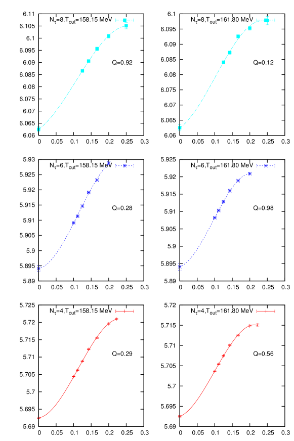
Figure 2: Pseudo transition couplings from maxima of the Polyakov loop susceptibility.

In our simulations we accommodate both layers in the SU(3) scaling region, so that (4) holds, which starts slightly below $\beta^{g}=5.65$. With our smallest $N_{\tau}=4$ temporal extension this sets the lower limit on $\beta^{g}_{\rm out}$. To work with round numbers we decided to start $N_{\tau}=4$ simulations at $\beta^{g}_{\rm out}=5.65$ and $\beta^{g}_{\rm out}=5.66$. Translated into temperatures this corresponds to $T_{\rm out}=158.15\,{\rm MeV}$ and $T_{\rm out}=161.80\,{\rm MeV}$. For larger $N_{\tau}=6$ and $N_{\tau}=8$ lattice these numbers have to be translated back into coupling constant values, listed in table 1 where we give an overview of the performed runs. The accuracy of the given numerical precision of the $T_{\rm out}$ values reflects the SU(3) scaling relation when translating back and forth, but has no significance for the accuracy of the physical temperature.

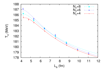
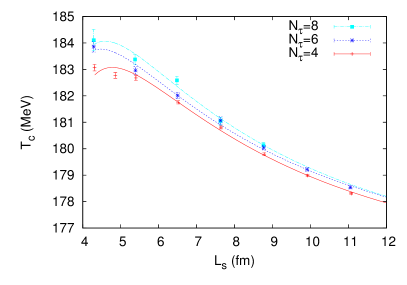
Figure 3: Pseudo transition temperatures versus volume edge length.

The small temperature difference between the confined phase and the infinite volume transition temperature makes it rather CPU time demanding to locate our deconfinment signals, the maxima of the Polyakov loop susceptibility. This is in essence overcome by brute force computer time. Relying on Fortran MPI code which is documented in [4], the bulk of our production was run at NERSC on their Cray XT4 and (more recently) Cray XE6, while code development and very limited production was done at FSU. All our runs used a statistics of $2^{13}$ sweeps for equilibration and $2^{21}$ sweeps for data production to overcome the statistical noise. Improved measurements techniques were tried, but did not result in major CPU time gains. Production on a $4\times 32^{3}$ DLT used 1,024 processors and took 5.7 hrs in real time. Approximate run times on other lattices can be scaled from this.

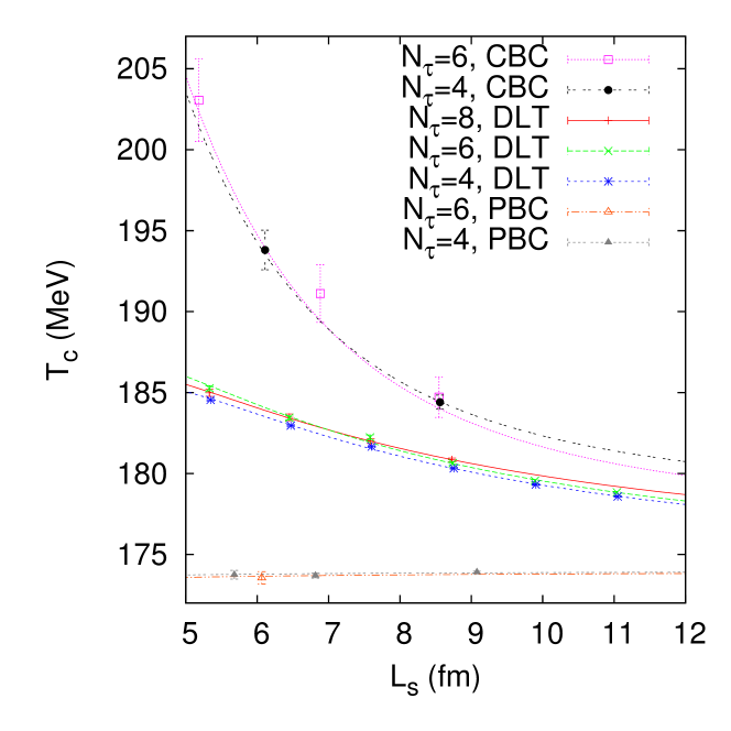
Figure 4: Pseudo transition temperatures versus volume edge length for CBC, DLT and PBC

Fig. 2 plots the raw data for pseudo transition couplings $\beta^{g}_{c}$ as determined from maxima of the Polyakov loop susceptibility and plotted versus the lattice ratio $N_{\tau}/N_{s}$ together with polynomial fits in $N_{\tau}/N_{s}$ up to order $(N_{\tau}/N_{s})^{3}$. For $N_{\tau}=4$ and $N_{\tau}=6$ we have excluded data from our smallest lattices, $N_{\tau}/N_{s}\leq 0.5$, because they suffer from peculiar finite size effects, which can be traced to the edges of the DLT layers. From down to up the lattices sizes are given by $N_{\tau}=4,\,6,\,8$. The corresponding $\beta^{g}$ ranges of pseudo transition temperatures shown in the figure increase from [5.69,5.725] ($N_{\tau}=4$) to [5.89,5.93] ($N_{\tau}=6$) to [6.06,6.11] ($N_{\tau}=8$). As seen in Fig. 3 the curves from these disconnected regions collapse into almost one curve when the SU(3) scaling relation (4) is applied to convert $\beta^{g}_{c}$ to $T_{c}$ in units of MeV, which we plot versus the volume edge length in fermi.

Our final Fig. 4 presents $T_{c}$ results for outside temperature $T_{\rm out}=158.15\,{\rm MeV}$ together with those of CBC from [2], where the strong coupling limit $\beta^{g}\to 0$ was used as BC. Even with our present high outside temperature the correction to the infinite volume critical temperature turns out to be remarkably large. So, this effect warrants further investigation. Instead of using a DLT one may incorporate cold boundaries by a surrounding region and, in particular, one may be interested in the inclusion of quarks in such calculations.

4 Summary and conclusions

• Even with a large outside temperature of about 160 MeV finite size correction of the SU(3) deconfining temperature due to small volumes are clearly visible.

• Our estimates of (pseudo) transition temperatures show SU(3) scaling behavior when increasing the temperature extension of the lattice from $N_{\tau}=4$ to $N_{\tau}=6$ and $N_{\tau}=8$.

• Small volumes increase the SU(3) transition temperature, while quark effects decrease it. If the increase holds also with quarks included, previous lattice calculations would underestimate the transition temperatures at RHIC.

Acknowledgments: We thank Alexei Bazavov for useful discussions. This work has in part been supported by DOE grant DE-FG02-97ER-41022. Most MCMC data were produced at NERSC under grant ERCAP 84105.

References

- [1] See the talk by Ludmila Levkova in these proceedings.
- [2] A. Bazavov and B.A. Berg, Phys. Rev. D 76, 014502 (2007).
- [3] C. Spieles, H. Stocker and C. Greiner, Phys. Rev. C 57, 908 (1998); A. Gopie and M.C. Ogilvie, Phys. Rev. D 59, 034009 (1999); J. Braun, B. Klein, H.J. Pirner and A.H. Rezaeian, Phys. Rev. D 73, 074010 (2006); L.M. Abreu, M. Gomes and A.J. da Silva, Phys. Lett. B 642, 551 (2006); N. Yamamoto and T. Kanazawa, Phys. Rev. Lett. 103, 032001 (2009); L.F. Palhares, E.S. Fraga and T. Kodam, J. Phys. G 37, 094031 (2010) and references therein.
- [4] B.A. Berg, arXiv:0904.0642; B.A. Berg and Hao Wu, arXiv:0904.1179.
- [5] B.A. Berg, A. Bazavov and Hao Wu, POS (LAT2009) 164.
- [6] G. Arnold, T. Lippert, T. Neuhaus and K. Schilling, Nucl. Phys. B (Proc. Suppl.) 94, 651 (2001) [hep-lat/0011058].
- [7] G. Boyd, J. Engels, F. Karsch, E. Laermann, C. Legeland, M. Lütgemeier and B. Peterson, Nucl. Phys. B 469 (1996) 419.
- [8] A. Bazavov, B.A. Berg and A. Velytsky, Phys. Rev. D 74 (2006) 014501.
- [9] S. Necco and R. Sommer, Nucl. Phys. B 622 (2002) 328.