Nested BDDC for a saddle-point problem

Abstract

We propose a Nested BDDC for a class of saddle-point problems. The method solves for both flux and pressure variables. The fluxes are resolved in three-steps: the coarse solve is followed by subdomain solves, and last we look for a divergence-free flux correction and pressure variables using conjugate gradients with a Multilevel BDDC preconditioner. Because the coarse solve in the first step has the same structure as the original problem, we can use this procedure recursively and solve (a hierarchy of) coarse problems only approximately, utilizing the coarse problems known from the BDDC. The resulting algorithm thus first performs several upscaling steps, and then solves a hierarchy of problems that have the same structure but increase in size while sweeping down the levels, using the same components in the first and in the third step on each level, and also reusing the components from the higher levels. Because the coarsening can be quite aggressive, the number of levels can be kept small and the additional computational cost is significantly reduced due to the reuse of the components. We also provide the condition number bound and numerical experiments confirming the theory.

1 Introduction

The Balancing Domain Decomposition by Constraints (BDDC), proposed independently by Cros Cros-2003-PSC , Dohrmann Dohrmann-2003-PSC , and Fragakis and Papadrakakis Fragakis-2003-MHP , is along with the Finite Element Tearing and Interconnecting - Dual, Primal (FETI-DP) method by Farhat et al. Farhat-2001-FDP ; Farhat-2000-SDP currently one of the most advanced and popular methods of iterative substructuring. These methods have been derived by modifications of the BDD method by Mandel Mandel-1993-BDD , and of the FETI method by Farhat and Roux Farhat-1991-MFE , respectively. The relations between these two families of methods have been studied extensively by many analysts in the substructuring field cf., e.g., Brenner-2007-BFW ; Li-2006-FBB ; Mandel-2005-ATP ; Mandel-2007-BFM , and also Sousedik-2008-CDD . The methods have been also extended to multiple levels: one can find multilevel extensions of the BDDC in Mandel-2008-MMB ; Sousedik-2010-AMB-thesis ; Sousedik-2011-AMB ; Tu-2007-TBT3D ; Tu-2007-TBT and of FETI in Klawonn-2009-HA3 . Here, we will be interested in extensions to saddle-point problems, such as to the Stokes problem Li-2006-BAI ; Pavarino-2002-BNI ; Sistek-2011-APB and in particular to the flow in porous media. One of the first domain decomposition methods for mixed finite element problems were proposed by Glowinski and Wheeler Glowinski-1988-DDM . Their Method II has been preconditioned using BDD by Cowsar et al. Cowsar-1995-BDD and using BDDC by Tu Tu-2007-BAF . This approach is sometimes regarded as hybrid because the method iterates on a system of dual variables (as Lagrange multipliers) enforcing the continuity of flux variables across the substructure interfaces. However, in order to simplify a multilevel extension, we would like to retain the original primal variables, and therefore we find the recent work of Tu Tu-2005-BAM ; Tu-2011-TBA to be more relevant for our approach.

In this paper, we propose a Nested BDDC method, which is a generalization of the Multilevel BDDC into a larger algorithmic framework suited for a class of saddle-point problems. Our starting point is the algorithm of Ewing and Wang Ewing-1992-ASA , see also Mathew Mathew-1993-SAIa . The basic idea is to solve for flux variables in three-steps: first we perform a coarse solve which is followed by independent subdomain solves with zero boundary conditions in the second step. In the third step, we look for a flux correction and pressures. Due to the design of the algorithm, the flux correction is divergence-free, and we can use conjugate gradients (CG, resp. PCG) with a preconditioner that preserves all of the iterates in the divergence-free subspace. To this end we adapt the Multilevel BDDC preconditioner from Mandel-2008-MMB to saddle-point problems. Applications of the two-, resp. three-level BDDC in the third step of this algorithm have been studied by Tu in Tu-2005-BAM ; Tu-2011-TBA . Also, one has to make a careful decision in the design of the coarse solve for the first step. A straightforward idea is to use the same, but “coarse” finite element discretization and a natural (linear) interpolation between the two meshes as considered in Mathew-1993-SAIa ; Tu-2005-BAM . Alternatively, the coarse solve has been obtained by an action of the BDDC preconditioner on a carefully chosen vector by Tu in Tu-2006-BDD ; Tu-2011-TBA and she has also numerically observed a very similar performance of the two choices (Tu-2006-BDD, , Section 4.8). Obviously, we favor here the second idea. Next, noting that the coarse solve in the first step has the same structure as the original problem, we can use the algorithm recursively, and solve a hierarchy of coarse solves only approximately. The resulting algorithm of the Nested BDDC thus first creates a hierarchy of (coarse) problems with similar structure scaling-up through the levels. Then this hierarchy is solved, while sweeping down the levels in a loop of outer iterations, using the same components in the first and the third step on each level, and also reusing the components from all of the previous (higher) levels. Because the coarsening can be quite aggressive, the number of levels can be kept small and the additional computational cost is significantly reduced due to the reusing of components. From this perspective our method can be viewed as a way of numerical upscaling via the coarse basis functions known from the BDDC. Therefore, unlike some of the previous works, we do not use the global partially assembled matrices neither the change of variables.

It is important to note that for the solution of closely related Stokes problem, the algorithm is reduced to step three because the solution itself is divergence-free. We also remark that the present approach is limited by a special choice of finite elements. In particular, we will work with the lowest-order Raviart-Thomas (RT0) elements that have piecewise constant basis functions for pressure variables. This is not the case when, e.g., Taylor-Hood elements are used and the BDDC preconditioned operator is no longer invariant on the divergence-free subspace Sistek-2011-APB . Finally, we note that our framework allows for irregular mesh decompositions, heterogeneous coefficients possibly utilizing the adaptive approach as in Mandel-2007-ASF ; Sousedik-2010-AMB-thesis , and also allows for a relatively straightforward extension into 3D. However, such extensions will be studied elsewhere.

The paper is organized as follows. In Section 2 we introduce the model problem, in Section 3 we introduce its mixed finite element discretization and recall the original algorithm of Ewing and Wang. In Section 4 we derive the two-level version of this algorithm using the BDDC components. In Section 5 we formulate the Nested BDDC method. In Section 6 we derive the condition number bound for the model problem, and finally in Section 7 we report on numerical experiments with a particular application to flow in porous media.

Throughout the paper we find it more convenient to work with abstract finite-dimensional spaces and linear operators between them instead of the space $\mathbb{R}^{n}$ and matrices. The results can be easily converted to the matrix language by choosing a finite element basis. For a symmetric positive definite bilinear form$~{}a$, we will denote the energy norm by $\left\|u\right\|_{a}=\sqrt{a\left(u,u\right)}$.

2 Model problem

Let $\Omega$ be a bounded polygonal domain in $\mathbb{R}^{n}$, $n=2$. Let us consider the following scalar, second-order, elliptic problem given as

$$-\nabla\cdot k\nabla p=f,\quad\text{in }\Omega,$$ (1)

where $k$ is a symmetric, uniformly positive definite matrix with bounded coefficients, the right-hand side $f\in L^{2}\left(\Omega\right)$, subject to sufficiently smooth boundary data on $\partial\Omega=\overline{\Gamma}_{E}\cup\overline{\Gamma}_{N}$. Equation (1) describes, e.g., a pressure field in an aquifer and therefore the variable $p$ will be called pressure. However, in reservoir simulations we are often interested in computing $-k\nabla p$ directly.

Introducing the so-called flux variable

$$\mathbf{u}=-k\nabla p,$$ (2)

we may rewrite (1) as a first-order system, generally known as Darcy’s problem,

$$k^{-1}\mathbf{u}+\nabla p =0,\quad\text{in }\Omega,$$

$$\nabla\cdot\mathbf{u} =f,\quad\text{in }\Omega,$$

$$p =g_{N},\quad\text{on }\Gamma_{N},$$

$$\mathbf{u}\cdot\mathbf{n} =g_{E},\quad\text{on }\Gamma_{E},$$

where $\mathbf{n}$ is the unit outward normal of $\Omega$, and for the boundary conditions it holds that $g_{N}\in H^{1/2}\left(\Gamma_{N}\right)$,  and $g_{E}\in H_{00}^{-1/2}\left(\Gamma_{E}\right)$. Without loss of generality, we will consider $\Gamma_{N}=\emptyset$. This case requires a compatibility condition

$$\int_{\Omega}f\,dx+\int_{\partial\Omega}g_{E}\,ds=0,$$ (3)

and the pressure $p$ will be determined uniquely up to an additive constant. Let us also for simplicity assume that $g_{E}=0$, and let us define a space

$$\mathbf{H}_{0}(\Omega;\operatorname{div})=\left\{\mathbf{v:v}\in L^{2}(\Omega);\nabla\cdot\mathbf{v}\in L^{2}(\Omega)\mathbf{\quad}\text{and}\mathbf{\quad v}\cdot\mathbf{n}=0\;\text{on }\partial\Omega\right\},$$ (4)

equipped with the norm

$$\left\|v\right\|_{\mathbf{H}_{0}(\Omega;\operatorname{div})}^{2}=\left\|\mathbf{v}\right\|_{L^{2}(\Omega)}^{2}+H_{\Omega}^{2}\left\|\nabla\cdot\mathbf{v}\right\|_{L^{2}(\Omega)}^{2},$$

where $H_{\Omega}$ denotes the characteristic size of $\Omega$, and the space

$$L_{0}^{2}(\Omega)=\left\{q:q\in L^{2}(\Omega)\mathbf{\quad}\text{and}\mathbf{\quad}\int_{\Omega}q\,dx=0\right\}.$$

The weak form of the Darcy’s problem, we would like to solve, is

$$\int_{\Omega}k^{-1}\mathbf{u}\cdot\mathbf{v}\,dx-\int_{\Omega}p\nabla\cdot\mathbf{v}\,dx =0,\quad\forall\mathbf{v}\in\mathbf{H}_{0}(\Omega;\operatorname{div}),$$ (5)

$$-\int_{\Omega}\nabla\cdot\mathbf{u}q\,dx =-\int_{\Omega}fq\,dx,\quad\forall q\in L_{0}^{2}\left(\Omega\right).$$ (6)

We refer to the monographs Brezzi-1991-MHF ; Toselli-2005-DDM for additional details.

3 Mixed finite elements and basic algorithm

Let $U$ be the lowest order Raviart-Thomas finite element space with a zero normal component on $\partial\Omega$ and $Q$ be a space of piecewise constants with a zero mean on $\Omega$. These two spaces, defined on the triangulation $\mathcal{T}_{h}$ of $\Omega$ where $h$ denotes the mesh size, are finite-dimensional subspaces of $\mathbf{H}_{0}(\Omega;\operatorname{div})$ and $L_{0}^{2}(\Omega)$, respectively, and they satisfy a uniform inf-sup condition, see Brezzi-1991-MHF .

Let us define the bilinear forms and the right-hand side by

$$a\left(u,v\right) =\int_{\Omega}k^{-1}\mathbf{u}\cdot\mathbf{v}\,dx,$$ (7)

$$b\left(u,q\right) =-\int_{\Omega}\nabla\cdot\mathbf{u}q\,dx,$$ (8)

$$\left\langle f,q\right\rangle =-\int_{\Omega}fq\,dx.$$ (9)

In the mixed variational formulation of the Darcy’s problem, eq. (5)-(6), we would like to find a pair $\left(u,p\right)\in\left(U,Q\right)$ such that

$$a\left(u,v\right)+b\left(v,p\right) =0,\qquad\forall v\in U,$$ (10)

$$b\left(u,q\right) =\left\langle f,q\right\rangle,\qquad\forall q\in Q.$$ (11)

Let us split the domain $\Omega$ into non-overlapping subdomains $\Omega_{i}$, $i=1,\dots,N$, assuming further that they form a triangulation of$~{}\Omega$, e.g., for a moment as macroelements. Accordingly, let us split the solution spaces as

$$U =U_{0}+\left(\oplus_{i=1}^{N}U_{i}\right)+U_{\text{corr}},$$ (12)

$$Q =\oplus_{i=0}^{N}Q_{i}.$$ (13)

The spaces $U_{0}$, $Q_{0}$ are obtained by considering subdomains as macroelements. The spaces $U_{i}$, $Q_{i}$, for $i=1,\dots,N$, are obtained by a restriction from the global solution spaces $U$, $Q$. More specifically, because $U_{I}=\oplus_{i=1}^{N}U_{i}$, the functions from $U_{i}$ have vanishing normal components (i.e., zero fluxes) along the subdomain interfaces. Also, in order to determine the pressure $p$ uniquely, we will consider the component $p_{0}\in Q_{0}$, which is constant in each subdomain$~{}\Omega_{i}$, to have a zero average over the whole domain $\Omega$, and the components $p_{i}\in Q_{i}$ to have zero averages over the subdomain $\Omega_{i}$ and identically equal to zero in other subdomains. The introduction of the auxiliary space $U_{\text{corr}}=U$ is motivated by an observation that in general

$$U\neq U_{0}+\left(\oplus_{i=1}^{N}U_{i}\right),$$ (14)

because the fluxes on subdomain interfaces might not be constant. We note that we will take an advantage of this splitting, in particular because for all $u_{I}\in U_{I}$ and $q_{0}\in Q_{0}$, it holds, by the divergence theorem, that

$$b\left(u_{I},q_{0}\right)=-\int_{\Omega}\left(\nabla\cdot u_{I}\right)\,q_{0}\,dx=0.$$ (15)

The following algorithm is due to Ewing and Wang Ewing-1992-ASA , cf. also Mathew Mathew-1993-SAIa .

Algorithm 3.1 (Basic)

Find the pair $\left(u,p\right)\in\left(U,Q\right)$ that satisfies (10)-(11) as

$$u=u_{0}+\sum_{i=1}^{N}u_{i}+u_{\text{corr}},$$

in the following three steps: Compute

1. the coarse component $\left(u_{0},p_{0}\right)\in\left(U_{0},Q_{0}\right)$ by solving

   $$a\left(u_{0},v_{0}\right)+b\left(v_{0},p_{0}\right) =0,\qquad\forall v_{0}\in U_{0},$$ (16)

   $$b\left(u_{0},q_{0}\right) =\left\langle f,q_{0}\right\rangle,\qquad\forall q_{0}\in Q_{0}.$$ (17)

   Note that because $Q_{0}\varsubsetneq Q$, in general

   $$b\left(u_{0},q\right)\neq\left\langle f,q\right\rangle,\qquad\forall q\in Q.$$

2. the substructure components $\left(u_{i},p_{i}\right)\in\left(U_{i},Q_{i}\right)$ for $i=1,\dots,N$ from

   $$a\left(u_{i},v_{i}\right)+b\left(v_{i},p_{i}\right) =-a\left(u_{0},v_{i}\right),\qquad\forall v_{i}\in U_{i},$$

   $$b\left(u_{i},q_{i}\right) =\left\langle f,q_{i}\right\rangle-b\left(u_{0},q_{i}\right),\qquad\forall q_{i}\in Q_{i}.$$

   Add the computed solutions as

   $$u^{\ast}=u_{0}+\sum_{i=1}^{N}u_{i}.$$

   Due to the correction in the second step, and with respect to (13), we obtain

   $$b\left(u^{\ast},q\right)=\left\langle f,q\right\rangle,\qquad\forall q\in Q.$$ (18)

   On the other hand, from (14), in general $u^{\ast}\neq u$. Therefore, we also need

3. the correction $u_{\text{corr}}\in U_{\text{corr}}=U$. Considering

   $$u=u^{\ast}+u_{\text{corr}},$$

   substituting into (10)-(11) and using (18), compute $\left(u_{\text{corr}},p\right)\in\left(U,Q\right)$ from

   $$a\left(u_{\text{corr}},v\right)+b\left(v,p\right) =-a\left(u^{\ast},v\right),\qquad\forall v\in U,$$

   $$b\left(u_{\text{corr}},q\right) =0,\qquad\forall q\in Q.$$

Remark 1

We would like to accentuate the reduction effect of Algorithm 3.1: the structural difference between problem (10)-(11) and the problem in Step 3 of Algorithm 3.1 is that the right-hand side of the reduced problem has a vanishing second component, which corresponds to the divergence-free subspace. Also, because the pressure components $p_{0}$, $p_{I}$ computed in Step 1 and Step 2, resp., are tested only against proper subspaces of $U$, we simply disregard them.

The application of the BDDC preconditioner for the computation of $u_{\text{corr}}$ for the two-, resp. three-level BDDC method has been studied by Tu Tu-2005-BAM ; Tu-2011-TBA . However, comparing (16)-(17) with (10)-(11), we see that in fact we can use the same algorithm recursively, with multiple levels, to solve for both $u_{0}$ and $u_{\text{corr}}$. But first, let us reformulate the basic Algorithm 3.1 with BDDC components.

4 Basic algorithm with BDDC components

We begin by introducing the substructuring components. Let $\Omega$ be decomposed into nonoverlapping subdomains $\Omega_{i}$, $i=1,\ldots,N,$ also called substructures, forming a quasi-uniform triangulation of $\Omega$ with the characteristic subdomain size $H$. Each substructure is a union of the lowest order Raviart-Thomas (RT0) finite elements with a matching discretization across the substructure interfaces. Let $\Gamma_{i}=\partial\Omega_{i}\backslash\partial\Omega$ be the set of boundary degrees of freedom of the substructure$~{}\Omega_{i}$ shared with other substructures$~{}\Omega_{j}$, $j\neq i$, and let us define the interface by $\Gamma=\cup_{i=1}^{N}\Gamma_{i}$. Let us denote by $\mathcal{F}$ the set of all faces between substructures, i.e., in the present context the set of all intersections $\Gamma_{ij}=\Gamma_{i}\cap\Gamma_{j}$, $i\neq j$. Note that with respect to our discretization we define only faces, but no corners (nor edges in 3D) known from other types of substructuring. Let us also slightly generalize the settings by allowing for constant coefficients $k_{i}$ in each subdomain$~{}\Omega_{i}$ separately.

Let us consider, cf. eq. (13), the decomposition of the pressure space

$$Q=Q_{0}\oplus Q_{I}\text{,\quad and\quad}Q_{I}=Q_{1}\times\dots\times Q_{N},$$ (19)

where $Q_{0}$ consists of constant functions in each subdomain, such that

$$\int_{\Omega}q_{0}\,dx=0,\quad\forall q_{0}\in Q_{0},\quad\text{and}\quad\int_{\Omega_{i}}q_{i}\,dx=0,\quad\forall q_{i}\in Q_{i},\;i=1,\dots,N.$$

Again, the space $Q$ is a finite-dimensional subspace of $L^{2}_{0}\left(\Omega\right)$, and therefore the unique solvability of all subsequently considered mixed problems is guaranteed.

Next, let $W_{i}$ be the space of the flux finite element functions on a substructure $\Omega_{i}$ such that all of their degrees of freedom on $\partial\Omega_{i}\cap\partial\Omega$ are zero, and let

$$W=W_{1}\times\dots\times W_{N}.$$

Now $U\subset W$ can be viewed as the subspace of all functions from $W$ continuous across substructure interfaces. Define $U_{I}\subset U$ as the subspace of functions that are zero on the interface $\Gamma$, i.e., the space of “interior” functions and let us define a projection$~{}P:w\in W\longmapsto\left(u_{I},p_{I}\right)\in\left(U_{I},Q_{I}\right)$ such that

$$a\left(u_{I},v_{I}\right)+b\left(v_{I},p_{I}\right) =a\left(w,v_{I}\right),\quad\forall v_{I}\in U_{I},$$

$$b\left(u_{I},q_{I}\right) =b\left(w,q_{I}\right),\quad\forall q_{I}\in Q_{I}.$$

Let us also define a projection$~{}P_{a}:w\in W\longmapsto u_{I}\in U_{I}\$ such that

$$a\left(u_{I},v_{I}\right)=a\left(w,v_{I}\right),\quad\forall v_{I}\in U_{I}.$$

Functions from the nullspace of $P$ and $P_{a}$ will be called Stokes harmonic and discrete harmonic, respectively. The following comparison of their energies, cf. (Toselli-2005-DDM, , Lemma 9.10), will allow us to apply some arguments from the scallar elliptic theory in Mandel-2008-MMB to the saddle-point problem considered here.

Lemma 1

Let $w\in W$. Then,

$$c\left\|\left(I-P\right)w\right\|_{a}\leq\left\|\left(I-P_{a}\right)w\right\|_{a}\leq\left\|\left(I-P\right)w\right\|_{a}.$$

Next, let $\widehat{W}$ be the space of all Stokes harmonic functions that are continuous across substructure interfaces, and such that

$$U=U_{I}\oplus\widehat{W},\quad\text{and\quad}U_{I}\perp_{a}\widehat{W}.$$ (20)

The first step in substructuring is typically the reduction of the problem to the interfaces. In particular, let us consider Step 3 of Algorithm 3.1, which can be written a bit more generally as: find a pair $\left(u,p\right)\in\left(U,Q\right)$ such that

$$a\left(u,v\right)+b\left(v,p\right) =\left\langle f^{\ast},v\right\rangle,\quad\forall v\in U,$$ (21)

$$b\left(u,q\right) =0,\quad\forall q\in Q.$$ (22)

The problem (21)-(22) can be reduced to finding $\left(\widehat{w},p_{0}\right)\in\left(\widehat{W},Q_{0}\right)$ such that

$$a\left(\widehat{u},\widehat{v}\right)+b\left(\widehat{v},p_{0}\right) =\left\langle f^{\ast},\widehat{v}\right\rangle,\quad\forall\widehat{v}\in\widehat{W},$$ (23)

$$b\left(\widehat{u},q_{0}\right) =0,\quad\forall q_{0}\in Q_{0}.$$ (24)

Such “reduction” is in implementation achieved by elimination of the interiors, known also as static condensation, see, e.g., (Toselli-2005-DDM, , Section 9.4.2) for more details. Now, let us define a subspace of balanced functions as

$$\widehat{W}_{B}=\left\{\widehat{v}\in\widehat{W}:b\left(\widehat{v},q_{0}\right)=0,\quad\forall q_{0}\in Q_{0}\right\}.$$ (25)

The problem (23)-(24) is equivalent to the following positive definite problem

$$\widehat{u}\in\widehat{W}_{B}:\quad a\left(\widehat{u},\widehat{v}\right)=\left\langle f^{\ast},\widehat{v}\right\rangle,\quad\forall\widehat{v}\in\widehat{W}_{B}.$$ (26)

Note that the space $U_{I}$ is balanced due to (15). Then, using $\widehat{W}_{B}$ in the splitting (20) implies that $U$ is also balanced in the sense of the definition (25).

The BDDC method is a two-level preconditioner characterized by the selection of certain coarse degrees of freedom. In the present setting these will be flux averages over each face, and pressure averages over each substructure, cf. Assumption 5.3. In particular, the value of a coarse degree of freedom will be taken as an average of the fine scale degrees of freedom. Next, let $\widetilde{W}\subset W$ be the subspace of all functions such that the values of any flux coarse degrees of freedom have a common value over a face shared by a pair of adjacent substructures, and vanish on $\partial\Omega$. Next, define $\widetilde{W}_{\Pi}\subset\widetilde{W}$ as the subspace of all functions such that their flux coarse degrees of freedom between pairs of adjacent substructures coincide, and such that they are Stokes harmonic, and let us also define $\widetilde{W}_{\Delta}\subset W$ as the subspace of all functions such that their flux coarse degrees of freedom vanish. Clearly, functions in $\widetilde{W}_{\Pi}$ are uniquely determined by the values of their flux coarse degrees of freedom, and

$$\widetilde{W}=\widetilde{W}_{\Delta}\oplus\widetilde{W}_{\Pi}.$$ (27)

Let $E$ be a projection from $\widetilde{W}$ onto $U$, defined by taking some weighted average of corresponding degrees of freedom on substructure interfaces, cf. Remark 2.

Remark 2

The entries in the matrix corresponding to the averaging operator$~{}E$ are given by scaling weights corresponding to a degree of freedom $x\in\Omega_{i}$ as

$$e_{i}(x)=\begin{cases}\frac{k_{i}^{-\gamma}}{k_{i}^{-\gamma}+k_{j}^{-\gamma}}&\mbox{if }x\in\partial\Omega_{i}\cap\partial\Omega_{j},\\ 1&\mbox{if }x\in\Omega_{i}\backslash\Gamma.\end{cases}$$

The case $\gamma=1$ corresponds to the so-called $\rho-$scaling, $\gamma=0$, i.e. $e_{i}\left(x\right)$ is $1/2$ or $1,$ corresponds to the multiplicity scaling, cf. Klawonn-2008-AFA . We note that the $\rho-$scaling is the same as the stiffness scaling because each flux degree of freedom is shared by two elements shared by at most a pair of subdomains.

Next, observe that it is only required for $u^{\ast}$ to satisfy (18). In particular, we do not need the substructures to form the same discretization as on the finite element level. Instead, we can conveniently retain the algebraic framework of the BDDC method introduced above and use its coarse problem in place of the coarse solve in Step 1. Specifically, let us set $U_{0}=\widetilde{W}_{\Pi}$. We are now ready to take the second look at Algorithm 3.1 and formulate its first modification.

Algorithm 4.1 (Basic algorithm with BDDC components)

Find the solution $\left(u,p\right)\in\left(U,Q\right)$ of the problem (10)-(11) by computing:

1. the coarse component $u_{0}\in\widehat{W}:$ solving for $\left(\widetilde{w}_{0},p_{0}\right)\in\left(\widetilde{W}_{\Pi},Q_{0}\right)$ the system

   $$a\left(\widetilde{w}_{0},\widetilde{v}_{\Pi}\right)+b\left(\widetilde{v}_{\Pi},p_{0}\right) =0,\qquad\forall\widetilde{v}_{\Pi}\in\widetilde{W}_{\Pi},$$ (28)

   $$b\left(\widetilde{w}_{0},q_{0}\right) =\left\langle f,q_{0}\right\rangle,\qquad\forall q_{0}\in Q_{0},$$ (29)

   dropping $p_{0}$, and applying the projection

   $$u_{0}=E\widetilde{w}_{0}.$$

2. the substructure components $\left(u_{I},p_{I}\right)\in\left(U_{I},Q_{I}\right)$ solving

   $$a\left(u_{I},v_{I}\right)+b\left(v_{I},p_{I}\right) =-a\left(u_{0},v_{I}\right),\qquad\forall v_{I}\in U_{I},$$

   $$b\left(u_{I},q_{I}\right) =\left\langle f,q_{I}\right\rangle-b\left(u_{0},q_{I}\right),\qquad\forall q_{I}\in Q_{I},$$

   dropping $p_{I}$, and combining the solutions $u^{\ast}=u_{0}+u_{I}.$

3. the correction and the pressure $\left(u_{\text{corr}},p\right)\in\left(U,Q\right)$ from

   $$a\left(u_{\text{corr}},v\right)+b\left(v,p\right) =-a\left(u^{\ast},v\right),\qquad\forall v\in U,$$

   $$b\left(u_{\text{corr}},q\right) =0,\qquad\forall q\in Q.$$

   Specifically, use the PCG method with the two-level BDDC preconditioner defined in Algorithm 4.2, using the coarse problem (28)-(29).

Finally, combine the three solutions as

$$u=u_{0}+u_{I}+u_{\text{corr}}.$$

Note that we again disregard the pressures $p_{0}$ and $p_{I}$ from Steps 1 and 2 as in Algorithm 3.1. The algorithm of the two-level BDDC preconditioner used in Step 3 is closely related to the original version for elliptic problems, cf. (Mandel-2008-MMB, , Algorithm 11). For completeness its version for saddle-point problems follows.

Algorithm 4.2 (Two-level BDDC preconditioner)

Define the preconditioner $\left(r,0\right)\in\left(U^{\prime},Q^{\prime}\right)\longmapsto\left(u,p\right)\in\left(U,Q\right)$ as follows:

Compute the interior pre-correction $\left(u_{I},p_{I}\right)\in\left(U_{I},Q_{I}\right)$ from

$$a\left(u_{I},z_{I}\right)+b\left(z_{I},p_{I}\right) =\left\langle r,z_{I}\right\rangle,\qquad\forall z_{I}\in U_{I},$$

$$b\left(u_{I},q_{I}\right) =0,\qquad\forall q_{I}\in Q_{I}.$$

Set up the updated residual

$$r_{B}\in U^{\prime},\quad\left\langle r_{B},v\right\rangle=\left\langle r,v\right\rangle-\left[a\left(u_{I},v\right)+b\left(v,p_{I}\right)\right],\qquad\forall v\in U.$$

Compute the substructure correction $w_{\Delta}\in\widetilde{W}_{\Delta}$ from

$$a\left(w_{\Delta},z_{\Delta}\right)+b\left(z_{\Delta},p_{I\Delta}\right) =\left\langle r_{B},Ez_{\Delta}\right\rangle,\qquad\forall z_{\Delta}\in\widetilde{W}_{\Delta},$$

$$b\left(w_{\Delta},q_{I}\right) =0,\qquad\forall q_{I}\in Q_{I}.$$

Compute the coarse correction $\left(w_{\Pi},p_{0}\right)\in\left(\widetilde{W}_{\Pi},Q_{0}\right)$ from

$$a\left(w_{\Pi},z_{\Pi}\right)+b\left(z_{\Pi},p_{0}\right) =\left\langle r_{B},Ez_{\Pi}\right\rangle,\qquad\forall z_{\Pi}\in\widetilde{W}_{\Pi},$$

$$b\left(w_{\Pi},q_{0}\right) =0,\qquad\forall q_{0}\in Q_{0}.$$

Add the averaged corrections

$$u_{B}=E\left(w_{\Delta}+w_{\Pi}\right).$$

Compute the interior post-correction $\left(v_{I},q_{I}\right)\in\left(U_{I},Q_{I}\right)$ from

$$a\left(v_{I},z_{I}\right)+b\left(z_{I},q_{I}\right) =a\left(u_{B},z_{I}\right),\quad\forall z_{I}\in U_{I},$$

$$b\left(v_{I},\overline{q}_{I}\right) =b\left(u_{B},\overline{q}_{I}\right),\quad\forall\overline{q}_{I}\in Q_{I}.$$

Apply the combined corrections

$$u =u_{I}+u_{B}-v_{I},$$

$$p =p_{I}+p_{0}-q_{I}.$$

Remark 3

The solve in the space $\widetilde{W}_{\Delta}$ gives rise to independent problems on substructures and the global coarse problem in the space $\widetilde{W}_{\Pi}$ is exactly the same as the one used in Step 1 of Algorithm 4.1.

We could implement Step 3 of Algorithm 4.1 by performing first the static condensation, iteratively solving the problem in the spaces $\left(\widehat{W},Q_{0}\right)$, and recovering the interiors after the convergence. This would remove the interior pre-, and post-corrections from Algorithm 4.2, cf. (Mandel-2008-MMB, , Algorithms 7, 9, 11), but performance of these two versions would be the same, cf. (Mandel-2008-MMB, , Theorem 14). Such approach might be also more appealing from the practical point of view, because it allows for iterations on a much smaller, Schur complement, system of linear equations see, e.g., (Toselli-2005-DDM, , Sections 4.3 and 9.4.2) for details. For a proof that given a sufficient number of constraints, the PCG method with the two-level BDDC preconditioner is invariant on the space of balanced, resp. divergence-free functions see (Tu-2005-BAM, , Lemma 2) or Lemma 3 in the next section.

In order to provide the condition number bound, let us introduce a larger space of balanced functions defined as

$$\widetilde{W}_{B}=\left\{v\in\widetilde{W}:b\left(v,q_{0}\right)=0,\quad\forall q_{0}\in Q_{0}\right\},$$

i.e., $\widehat{W}_{B}\subset\widetilde{W}_{B}$, and for which we get, using (4) and (7), the equivalence

$$c\left\|v\right\|_{a}^{2}\leq\left\|v\right\|_{\mathbf{H}_{0}(\Omega;\operatorname{div})}^{2}\leq C\left\|v\right\|_{a}^{2},\quad\forall v\in\widetilde{W}_{B}.$$ (30)

Due to the equivalence of the problems (21)-(22), (23)-(24) and (26), and with respect to the equivalence of norms (30) and Lemma 1, we can conveniently use the $a-$norm in the following estimate, and the condition number bound known from the elliptic case cf., e.g., (Mandel-2007-BFM, , Theorem 4) carries over.

Theorem 4.3 ((Tu-2005-BAM, , Lemma 8, Theorem 1))

The condition number $\kappa$ of the two-level BDDC preconditioner from Algorithm 4.2 satisfies the bound

$$\kappa\leq\omega=\max\left\{{\sup_{w\in\widetilde{W}_{B}}\frac{\left\|\left(I-P\right)Ew\right\|_{a}^{2}}{\left\|w\right\|_{a}^{2}},1}\right\}\text{ }\leq C\left(1+\log\frac{H}{h}\right)^{2}{.}$$ (31)

Remark 4

In (Tu-2005-BAM, , Lemma 8), the supremum was taken over the space $\left(I-P\right)\widetilde{W}_{B}$ of Stokes harmonic balanced function. Nevertheless, the bound remains the same by considering the larger space $\widetilde{W}_{B}$, cf. also (Mandel-2008-MMB, , Remark 16).

In Algorithm 4.1, the coarse problem used in Steps 1 and 3 is solved exactly, and therefore becomes a bottleneck in the case of many substructures. In the next section we will suggest its further modification by using it recursively for Step 1, on a multiple of different levels leading to the Nested BDDC method.

5 Nested BDDC

We extend Algorithm 4.1 to multiple levels by using it recursively for Step 1, leading to a multilevel decomposition, and introducing thus a loop of outer iterations with the size given by the number of different decomposition levels.

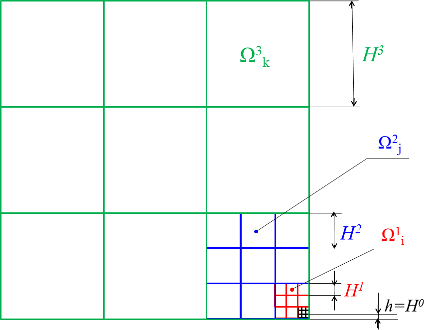
Figure 1: An example of a uniform decomposition for a four-level method with $H^{\ell}/H^{\ell-1}=3$.

$$\framebox{$\begin{array}[c]{ccccccccccccccc}&&Q&=&Q^{0}_{0}&&&&&&&&&&\\ &&\shortparallel&&&&&&&&&&&&\\ &&Q^{1}&=&Q^{1}_{0}&\oplus&Q^{1}_{I}&&&&&&&&\\ &&&&\shortparallel&&&&&&&&&&\\ &&&&Q^{2}&=&Q^{2}_{0}&\oplus&Q^{2}_{I}&&&&&&\\ &&&&&&\shortparallel&&&&&&&&\\ &&&&&&\vdots&&&&&&&&\\ &&&&&&\shortparallel&&&&&&&&\\ &&&&&&Q^{L-1}&=&Q^{L-1}_{0}&\oplus&Q^{L-1}_{I}&&&&\\ &&&&&&&&&&&&&&\\ &&U&=&\widetilde{W}_{\Pi}^{0}&&&&&&&&&&\\ &&\shortparallel&&&&&&&&&&&&\\ U_{I}^{1}&{\genfrac{}{}{0.0pt}{}{\genfrac{}{}{0.0pt}{}{P^{1}}{\leftarrow}}{\subset}}&U^{1}&{\genfrac{}{}{0.0pt}{}{\genfrac{}{}{0.0pt}{}{E^{1}}{\leftarrow}}{\subset}}&\widetilde{W}_{\Pi}^{1}&\oplus&\widetilde{W}_{\Delta}^{1}&=&\widetilde{W}^{1}&\subset&W^{1}&&&&\\ &&&&\shortparallel&&&&&&&&&&\\ &&U_{I}^{2}&{\genfrac{}{}{0.0pt}{}{\genfrac{}{}{0.0pt}{}{P^{2}}{\leftarrow}}{\subset}}&U^{2}&{\genfrac{}{}{0.0pt}{}{\genfrac{}{}{0.0pt}{}{E^{2}}{\leftarrow}}{\subset}}&\widetilde{W}_{\Pi}^{2}&\oplus&\widetilde{W}_{\Delta}^{2}&=&\widetilde{W}^{2}&\subset&W^{2}&&\\ &&&&{\scriptstyle\ \downarrow I^{2}}&&\shortparallel&&&&&&&&\\ &&&&\widetilde{U}^{2}&&\vdots&&&&&&&&\\ &&&&&&\shortparallel&&&&&&&&\\ &&&&U_{I}^{L-1}&{\genfrac{}{}{0.0pt}{}{\genfrac{}{}{0.0pt}{}{P^{L-1}}{\leftarrow}}{\subset}}&U^{L-1}&{\genfrac{}{}{0.0pt}{}{\genfrac{}{}{0.0pt}{}{E^{L-1}}{\leftarrow}}{\subset}}&\widetilde{W}_{\Pi}^{L-1}&\oplus&\widetilde{W}_{\Delta}^{L-1}&=&\widetilde{W}^{L-1}&\subset&W^{L-1}\\ &&&&&&{\scriptstyle\ \downarrow I^{L-1}}&&\shortparallel&&&&&&\\ &&&&&&\widetilde{U}^{L-1}&&U^{L}&&&&&&\\ &&&&&&&&{\scriptstyle\ \downarrow I^{L}}&&&&&&\\ &&&&&&&&\widetilde{U}^{L}&&&&&&\end{array}$}$$

Figure 2: Space decompositions, embeddings and projections in the Nested and Multilevel BDDC for a saddle-point problem described in Algorithm 5.1 and Algorithm 5.2, respectively. Note that the spaces $\widetilde{W}_{\Pi}^{\ell}$, $\ell=1,\dots,L-1$ in the Multilevel BDDC are by (42) also balanced. However in order to guarantee that the output of the Multilevel BDDC preconditioner is also balanced, resp. divergence-free in the sense of eq. (22), we need to satisfy Assumption 5.3.

The substructuring components from Section 4 will be denoted by an additional superscript ${}^{1},$ as $\Omega_{i}^{1},$ $i=1,\ldots N^{1}$, etc., and called level $1$. In particular, the problem (10)-(11) will be denoted as: find $\left(u^{1},p^{1}\right)\in\left(U^{1},Q^{1}\right)$ such that

$$a\left(u^{1},v^{1}\right)+b\left(v^{1},p^{1}\right) =0,\qquad\forall v^{1}\in U^{1},$$ (32)

$$b\left(u^{1},q^{1}\right) =\left\langle f^{1},q^{1}\right\rangle,\qquad\forall q^{1}\in Q^{1},$$ (33)

The level $1$ coarse problem solved in (28)-(29) will be called the level $2$ problem. It has the same finite element structure as the original problem (10)-(11) on level $1$, so we put $\widetilde{W}_{\Pi}^{1}=U^{2}$ and $Q_{0}^{1}=Q^{2}$. Level $1$ substructures are level $2$ elements and level $1$ coarse degrees of freedom are level $2$ degrees of freedom. Repeating this process recursively, level $\ell-1$ substructures become level $\ell$ elements, and the level $\ell$ substructures are agglomerates of level $\ell$ elements. An $L-$level method is thus given by nested decomposition levels $\ell=1,\dots,L-1$. Level $\ell$ substructures are denoted by $\Omega_{i}^{\ell},$ $i=1,\ldots,N^{\ell},$ and they are assumed to form a conforming triangulation with a characteristic substructure size $H^{\ell}$. An example of a decomposition is in Figure 1. For convenience, we denote by $\Omega_{i}^{0}$ the original finite elements and put $H^{0}=h$. The interface$~{}\Gamma^{\ell}$ on level$~{}\ell$ is defined as the union of all level$~{}\ell$ boundary degrees of freedom, i.e., degrees of freedom shared by at least two level$~{}\ell$ substructures, and we note that $\Gamma^{\ell}\subset\Gamma^{\ell-1}$. Level$~{}\ell-1$ coarse degrees of freedom become level$~{}\ell$ degrees of freedom. The shape functions on level $\ell$ are Stokes harmonic with respect to level $\ell-1$ shape functions, subject to the value of exactly one level$~{}\ell$ degree of freedom being one and others level$~{}\ell$ degrees of freedom being zero. We remark that as before the coarse degrees of freedom will be the flux averages over each face, and pressure averages over each substructure, cf. Assumption 5.3. The (Stokes harmonic) projection is performed on each level$~{}\ell$ element (level$~{}\ell-1$ substructure) separately, so the values of level$~{}\ell-1$ degrees of freedom are in general discontinuous between level$~{}\ell-1$ substructures, and only the values of level$~{}\ell$ degrees of freedom between neighboring level $\ell$ elements coincide.

The development of the spaces on level $\ell$ now parallels the finite element setting in Section 4, see also (Mandel-2008-MMB, , Section 6). First, let us consider similarly as before, cf. eq. (19), the recursive decomposition of the pressure spaces

$$Q^{\ell}=Q_{0}^{\ell}\oplus Q_{I}^{\ell}\text{,\quad and\quad}Q_{I}^{\ell}=Q_{1}^{\ell}\times\cdots\times Q_{N^{\ell}}^{\ell},\text{\qquad}\ell=1,\dots,L-1,$$ (34)

where $Q_{0}^{\ell}$ consists of constant functions in each level $\ell$ substructure, such that

$$\int_{\Omega^{\ell}}q_{0}^{\ell}\,dx=0,\quad\forall q_{0}^{\ell}\in Q_{0}^{\ell},\quad\text{and}\quad\int_{\Omega_{i}^{\ell}}q_{i}^{\ell}\,dx=0,\quad\forall q_{i}^{\ell}\in Q_{i}^{\ell},\;i=1,\dots,N^{\ell}.$$

Next, denote $U^{\ell}=\widetilde{W}_{\Pi}^{\ell-1}$. Let $W_{i}^{\ell}$ be the space of the flux functions on the substructure $\Omega_{i}^{\ell}$, such that all of their degrees of freedom on $\partial\Omega_{i}^{\ell}\cap\partial\Omega$ are zero, and on each decomposition level$~{}\ell=1,\dots,L-1,$ let

$$W^{\ell}=W_{1}^{\ell}\times\cdots\times W_{N^{\ell}}^{\ell}.$$

Now $U^{\ell}\subset W^{\ell}$ can be viewed as the subspace of all functions from$~{}W^{\ell}$ that are continuous across the interface $\Gamma^{\ell}$. Define $U_{I}^{\ell}\subset U^{\ell}$ as the subspace of functions that are zero on$~{}\Gamma^{\ell}$, i.e., the functions “interior” to the level$~{}\ell$ substructures. Define projections $P^{\ell}$:$w^{\ell}\in W^{\ell}\longmapsto\left(u_{I}^{\ell},p_{I}^{\ell}\right)\in\left(U_{I}^{\ell},Q_{I}^{\ell}\right)$ such that

$$a\left(u_{I}^{\ell},v_{I}^{\ell}\right)+b\left(v_{I}^{\ell},p_{I}^{\ell}\right) =a\left(w^{\ell},v_{I}^{\ell}\right),\quad\forall v_{I}^{\ell}\in U_{I}^{\ell}$$

$$b\left(u_{I}^{\ell},q_{I}^{\ell}\right) =b\left(w^{\ell},q_{I}^{\ell}\right),\quad\forall q_{I}^{\ell}\in Q_{I}^{\ell}.$$

Functions from the nullspace of $P^{\ell}$ will be called Stokes harmonic on level $\ell$. Next, let $\widehat{W}^{\ell}$ be the space of all Stokes harmonic functions that are continuous across substructure interfaces on level$~{}\ell$, and such that

$$U^{\ell}=U_{I}^{\ell}\oplus\widehat{W}^{\ell},\quad\text{and\quad}U_{I}^{\ell}\perp_{a}\widehat{W}^{\ell}.$$ (35)

Let $\widetilde{W}^{\ell}\subset W^{\ell}$ be the subspace of all functions such that the values of any flux coarse degrees of freedom on level$~{}\ell$ have a common value over a face shared by a pair of adjacent level$~{}\ell$ substructures and vanish on $\partial\Omega_{i}^{\ell}\cap\partial\Omega$. Define $\widetilde{W}_{\Pi}^{\ell}\subset\widetilde{W}^{\ell}$ as the subspace of all functions such that their level $\ell$ flux coarse degrees of freedom between adjacent substructures coincide, and such that they are Stokes harmonic, and let us also define $\widetilde{W}_{\Delta}^{\ell}\subset W^{\ell}$ as the subspace of all functions such that their level $\ell$ flux coarse degrees of freedom vanish. Clearly, functions in $\widetilde{W}_{\Pi}^{\ell}$ are uniquely determined by the values of their level$~{}\ell$ coarse degrees of freedom, and

$$\widetilde{W}^{\ell}=\widetilde{W}_{\Delta}^{\ell}\oplus\widetilde{W}_{\Pi}^{\ell}.$$ (36)

Let $E^{\ell}$ be a projection from $\widetilde{W}^{\ell}$ onto $U^{\ell}$, defined by taking some weighted average of corresponding coarse degrees of freedom on$~{}\Gamma^{\ell}$, cf. Remark 2.

These spaces and operators are used in both, Nested and Multilevel BDDC, algorithms described below. Their hierarchy is shown concisely in Figure 2. We are now ready to generalize the two-level Algorithm 4.1 to multiple levels.

Algorithm 5.1 (Nested BDDC)

Find the solution $\left(u^{1},p^{1}\right)\in\left(U^{1},Q^{1}\right)$ of the problem (32)-(33) in the following steps:

for $\ell=1,\ldots L-1$,

•

Step 1: formulate the coarse problem as: find $\left(w_{\Pi}^{\ell},p_{0}^{\ell}\right)\in\left(\widetilde{W}_{\Pi}^{\ell},Q_{0}^{\ell}\right)$ such that

$$a\left(w_{\Pi}^{\ell},z_{\Pi}^{\ell}\right)+b\left(z_{\Pi}^{\ell},p_{0}^{\ell}\right) =0,\qquad\forall z_{\Pi}^{\ell}\in\widetilde{W}_{\Pi}^{\ell},$$ (37)

$$b\left(w_{\Pi}^{\ell},q_{0}^{\ell}\right) =\left\langle f^{\ell},q_{0}^{\ell}\right\rangle,\qquad\forall q_{0}^{\ell}\in Q_{0}^{\ell},$$ (38)

•

If $\ell=L-1$, solve the coarse problem directly, drop $p_{0}^{\ell}$, and set $u_{0}^{L-1}=w_{\Pi}^{L-1}$.

•

Else, set $U^{\ell+1}=\widetilde{W}_{\Pi}^{\ell}$ and set up the right-hand side of (38) for level $\ell+1$,

$$f^{\ell+1}\in Q^{\ell+1\prime},\quad\left\langle f^{\ell+1},q^{\ell+1}\right\rangle=\left\langle f^{\ell},q^{\ell+1}\right\rangle,\qquad\forall q^{\ell+1}\in Q^{\ell+1},$$

end

for $\ell=L-1,\ldots 1$,

•

Step 2: find the substructure components $\left(u_{I}^{\ell},p_{I}^{\ell}\right)\in\left(U_{I}^{\ell},Q_{I}^{\ell}\right)$ from

$$a\left(u_{I}^{\ell},v_{I}^{\ell}\right)+b\left(v_{I}^{\ell},p_{I}^{\ell}\right) =-a\left(u_{0}^{\ell},v_{I}^{\ell}\right),\qquad\forall v_{I}^{\ell}\in U_{I}^{\ell},$$

$$b\left(u_{I}^{\ell},q_{I}^{\ell}\right) =\left\langle f^{\ell},q_{I}^{\ell}\right\rangle-b\left(u_{0}^{\ell},q_{I}^{\ell}\right),\qquad\forall q_{I}^{\ell}\in Q_{I}^{\ell},$$

drop $p_{I}^{\ell}$, and combine the two solutions

$$u^{\ast,\ell}=u_{0}^{\ell}+u_{I}^{\ell}.$$

•

Step 3: find the correction and the pressure $\left(u_{\text{corr}}^{\ell},p^{\ell}\right)\in\left(U^{\ell},Q^{\ell}\right)$ from

$$a\left(u_{\text{corr}}^{\ell},v^{\ell}\right)+b\left(v^{\ell},p^{\ell}\right) =-a\left(u_{0}^{\ast,\ell},v^{\ell}\right),\qquad\forall v^{\ell}\in U^{\ell},$$

$$b\left(u_{\text{corr}}^{\ell},q^{\ell}\right) =0,\qquad\forall q^{\ell}\in Q^{\ell}.$$

Specifically, use the PCG method with the Multilevel BDDC preconditioner defined in Algorithm 5.2, using the hierarchy of coarse problems (37)-(38).

•

Finally, combine the three solutions as

$$u^{\ell}=u_{0}^{\ell}+u_{I}^{\ell}+u_{\text{corr}}^{\ell}.$$

•

If $\ell>1$, drop $p^{\ell}$, and set $u_{0}^{\ell-1}=u^{\ell}$.

end

We note that the first loop provides a natural approach of scaling-up through the levels. The Multilevel BDDC preconditioner used in Step 3 of Algorithm 5.1 consists of recursive application of the two-level BDDC preconditioner for the approximate solution of the hierarchy of the coarse problems that were pre-computed in Step 1. Even though the preconditioner differs only little from its original version for elliptic problems described in (Mandel-2008-MMB, , Algorithm 17), we again include its saddle-point version here for completeness.

Algorithm 5.2 (Multilevel BDDC preconditioner)

Define the preconditioner $\left(r^{\ell},0\right)\in\left(U^{\ell\prime},Q^{\ell\prime}\right)\longmapsto\left(u^{\ell},p^{\ell}\right)\in\left(U^{\ell},Q^{\ell}\right)$ as follows:

for $k=\ell,\ldots,L-1$,

•

Compute the interior pre-correction $\left(u_{I}^{k},p_{I}^{k}\right)\in\left(U_{I}^{k},Q_{I}^{k}\right)$ from

$$a\left(u_{I}^{k},v_{I}^{k}\right)+b\left(v_{I}^{k},p_{I}^{k}\right) =\left\langle r^{k},v_{I}^{k}\right\rangle,\qquad\forall v_{I}^{k}\in U_{I}^{k},$$ (39)

$$b\left(u_{I}^{k},q_{I}^{k}\right) =0,\qquad\forall q_{I}^{k}\in Q_{I}^{k}.$$ (40)

•

Set up the updated residual

$$r_{B}^{k}\in U^{k\prime},\quad\left\langle r_{B}^{k},v^{k}\right\rangle=\left\langle r^{k},v^{k}\right\rangle-\left[a\left(u_{I}^{k},v^{k}\right)+b\left(v^{k},p_{I}^{k}\right)\right],\qquad\forall v^{k}\in U^{k}.$$

•

Compute the substructure correction $\left(w_{\Delta}^{k},p_{I\Delta}^{k}\right)\in\left(\widetilde{W}_{\Delta}^{k},Q_{I}^{k}\right)$ from

$$a\left(w_{\Delta}^{k},z_{\Delta}^{k}\right)+b\left(z_{\Delta}^{k},p_{I\Delta}^{k}\right) =\left\langle r_{B}^{k},E^{k}z_{\Delta}^{k}\right\rangle,\qquad\forall z_{\Delta}^{k}\in\widetilde{W}_{\Delta}^{k},$$

$$b\left(w_{\Delta}^{k},q_{I}^{k}\right) =0,\qquad\forall q_{I}^{k}\in Q_{I}^{k}.$$

•

Formulate the coarse problem as: find $\left(w_{\Pi}^{k},p_{0}^{k}\right)\in\left(\widetilde{W}_{\Pi}^{k},Q_{0}^{k}\right)$ such that

$$a\left(w_{\Pi}^{k},z_{\Pi}^{k}\right)+b\left(z_{\Pi}^{k},p_{0}^{k}\right) =\left\langle r_{B}^{k},E^{k}z_{\Pi}^{k}\right\rangle,\quad\forall z_{\Pi}^{k}\in\widetilde{W}_{\Pi}^{k},$$ (41)

$$b\left(w_{\Pi}^{k},q_{0}^{k}\right) =0,\quad\forall q_{0}^{k}\in Q_{0}^{k}.$$ (42)

•

If$\ k=L-1$, solve the coarse problem directly and set

$$u^{L} =w_{\Pi}^{L-1},$$

$$p^{L} =p_{0}^{L-1}.$$

•

Else, set $U^{k+1}=\widetilde{W}_{\Pi}^{k}$, set up the right-hand side $r^{k+1}$ of (39) for level$~{}k+1$,

$$r^{k+1}\in U^{k+1^{\prime}},\quad\left\langle r^{k+1},v^{k+1}\right\rangle=\left\langle r_{B}^{k},E^{k}v^{k+1}\right\rangle,\quad\forall v^{k+1}\in U^{k+1},$$

end

for $k=L-1,\ldots,\ell\mathbf{,}$ 

•

Average the approximate corrections,

$$u_{B}^{k} =E^{k}\left(w_{\Delta}^{k}+u^{k+1}\right),$$ (43)

$$p_{0}^{k} =p^{k+1}.$$ (44)

•

Compute the interior post-correction $\left(v_{I}^{k},q_{I}^{k}\right)\in\left(U_{I}^{k},Q_{I}^{k}\right)$ from

$$a\left(v_{I}^{k},z_{I}^{k}\right)+b\left(z_{I}^{k},q_{I}^{k}\right) =a\left(u_{B}^{k},z_{I}^{k}\right),\quad\forall z_{I}^{k}\in U_{I}^{k},$$ (45)

$$b\left(v_{I}^{k},\overline{q}_{I}^{k}\right) =b\left(u_{B}^{k},\overline{q}_{I}^{k}\right),\quad\forall\overline{q}_{I}^{k}\in Q_{I}^{k}.$$ (46)

•

Apply the combined corrections,

$$u^{k} =u_{I}^{k}+u_{B}^{k}-v_{I}^{k},$$ (47)

$$p^{k} =p_{I}^{k}+p_{0}^{k}-q_{I}^{k}.$$ (48)

end

In order to guarantee that the Multilevel BDDC preconditioner is invariant on the space of divergence-free functions, we will need the following:

Assumption 5.3

Suppose that the flux coarse degrees of freedom are prescribed as averages over every face on every decomposition level$~{}\ell$, $\ell=1,\dots,L-1$.

Lemma 2

Let Assumption 5.3 be satisfied. Then,

$$b\left(E^{\ell}w_{\Delta}^{\ell},q_{0}^{\ell}\right) =0,\quad\forall\left(w_{\Delta}^{\ell},q_{0}^{\ell}\right)\in\left(\widetilde{W}_{\Delta}^{\ell},Q_{0}^{\ell}\right),$$

$$b\left(E^{\ell}w_{\Pi}^{\ell},q_{0}^{\ell}\right) =b\left(w_{\Pi}^{\ell},q_{0}^{\ell}\right),\quad\forall\left(w_{\Pi}^{\ell},q_{0}^{\ell}\right)\in\left(\widetilde{W}_{\Pi}^{\ell},Q_{0}^{\ell}\right).$$

Proof

Note that with Assumption 5.3 satisfied, the values of coarse degrees of freedom of functions from the space $\widetilde{W}_{\Delta}^{\ell}$ are zero, i.e., the fine degrees of freedom have a zero average, and the values of coarse degrees of freedom for functions from the space $\widetilde{W}_{\Pi}^{\ell}$ for all (pairs of) adjacent substructures coincide. The claim now follows from the divergence theorem, because $q_{0}$ are piecewise constant in each level $\ell$ subdomain separately, cf. also (Tu-2005-BAM, , Lemma 2). ∎

Lemma 3

Let Assumption 5.3 be satisfied. Then the solution $u^{\ell}$ obtained from the Multilevel BDDC preconditioner in Algorithm 5.2 is divergence-free.

Proof

Let $\ell=1,\dots,L-1$ be fixed. Using (43), Lemma 2 and (42), we get

$$b\left(u_{B}^{\ell},q_{0}^{\ell}\right)=b\left(E^{\ell}w^{\ell},q_{0}^{\ell}\right)=b\left(w_{\Pi}^{\ell},q_{0}^{\ell}\right)=0,\quad\forall q_{0}^{\ell}\in Q_{0}^{\ell},$$ (49)

which also shows that $u_{B}^{\ell}\in\widehat{W}_{B}^{\ell}$. Next, using (47) and (34), we obtain

$$b\left(u^{\ell},q^{\ell}\right)=b\left(u_{I}^{\ell}+u_{B}^{\ell}-v_{I}^{\ell},q_{0}^{\ell}+q_{I}^{\ell}\right)=0,\quad\forall q^{\ell}\in Q^{\ell},$$

which follows using (15), (40), (46), and (49), i.e., $u^{\ell}$ is divergence-free. ∎

Thus with a careful choice of the initial solution, such that the residual corresponding to the substructure interiors and pressures is zero, the output of the Multilevel BDDC preconditioner is divergence-free and by induction all the PCG iterates, which are linear combinations of the initial error and the outputs of the preconditioner, stay in the divergence-free subspace.

In order to provide the condition number bound of the Multilevel BDDC for a saddle-point problem studied here, let us define, for levels $\ell=1,\dots,L-1$, a hierarchy of balanced spaces

$$\widetilde{W}_{B}^{\ell}=\left\{w^{\ell}\in\widetilde{W}^{\ell}:b\left(w^{\ell},q_{0}^{\ell}\right)=0,\quad\forall q_{0}^{\ell}\in Q_{0}^{\ell}\right\}.$$

The following condition number bound is a variant of (Mandel-2008-MMB, , Lemma 20).

Lemma 4

If for some $\omega^{\ell}\geq 1$,

$$\left\|(I-P^{\ell})E^{\ell}w^{\ell}\right\|_{a}^{2}\leq\omega^{\ell}\left\|w^{\ell}\right\|_{a}^{2},\quad\forall w^{\ell}\in\widetilde{W}_{B,}^{\ell}\quad\ell=1,\ldots,L-1,$$ (50)

then the Multilevel BDDC preconditioner (Algorithm 5.2) satisfies $\kappa\leq{\textstyle\prod_{\ell=1}^{L-1}}\omega^{\ell}.$

Proof

The bound was given for all $w^{\ell}\in$ $\widetilde{W}^{\ell}$ in the context of scalar elliptic problems in (Mandel-2008-MMB, , Lemma 20). Here, we need to show that for any $w^{\ell}\in\widetilde{W}_{B}^{\ell}$, the bilinear form $b$ will vanish also for the function on the left hand-side, i.e., that $\left(I-P^{\ell}\right)E^{\ell}w^{\ell}\in\widetilde{W}_{B}^{\ell}$. So, consider (36) and let $w^{\ell}=w_{\Delta}^{\ell}+w_{\Pi}^{\ell}$. Then

$$b\left(\left(I-P^{\ell}\right)E^{\ell}w^{\ell},q_{0}^{\ell}\right)=b\left(\left(I-P^{\ell}\right)w_{\Pi}^{\ell},q_{0}^{\ell}\right)=b\left(w_{\Pi}^{\ell},q_{0}^{\ell}\right)=0,$$

which follows from Lemma 2, definition of $P^{\ell}$ and (15), and from (42). ∎

6 Condition number bound for the model problem

We will now apply the methodology from Mandel-2008-MMB in order to derive a condition number bound for the model problem with the lowest order Raviart-Thomas dicretization. The key is the lower bound derived by Tu Tu-2011-TBA , which is limited to a geometric decomposition of the domain $\Omega$ on every decomposition level. In particular, let us make the following:

Assumption 6.1

Each subdomain $\Omega_{i}^{\ell},$ $\ell=0,\dots,L-1$ and $i=1,\dots,N^{\ell}$ is quadrilateral. The subdomains also form on every decomposition level $\ell$ a quasi-uniform coarse mesh of the domain $\Omega$ with a characteristic mesh size $H^{\ell}$.

First, note that by (42), on each level $\ell=0,\dots,L-1$, the coarse basis functions are balanced, i.e., for all $w_{\Pi}\in\widetilde{W}_{\Pi}^{\ell}$ we have that

$$b\left(w_{\Pi},q_{0}\right)=0,\qquad\forall q_{0}\in Q_{0}^{\ell},$$

and we can use the $a-$norm, which is also equivalent to $L^{2}-$norm, on the space $\widetilde{W}_{\Pi}^{\ell}$. So, let $\left\|w\right\|_{a(\Omega_{i}^{\ell})}$ be the energy norm of a function $w\in\widetilde{W}_{\Pi}^{\ell}$, $\ell=1,\ldots,L-1,$ restricted to subdomain$~{}\Omega_{i}^{\ell},$ $i=1,\ldots N^{\ell}$, and let $\left\|w\right\|_{a}$ be the norm obtained by piecewise integration over each $\Omega_{i}^{\ell}$. To apply Lemma 4 to our model problem, we need to generalize the polylogarithmic estimate from Theorem 4.3 to coarse levels. To this end, let $I^{\ell+1}:\widetilde{W}_{\Pi}^{\ell}\rightarrow\widetilde{U}^{\ell+1}$ be an interpolation from the level$~{}\ell$ coarse degrees of freedom (i.e., level $\ell+1$ degrees of freedom) to functions in another space $\widetilde{U}^{\ell+1}$ and assume that, for all levels $\ell=1,\ldots,L-1,$ and level $\ell$ subdomains $\Omega_{i}^{\ell}$, $i=1,\ldots,N^{\ell},$ the interpolation satisfies for all $w\in\widetilde{W}_{\Pi}^{\ell}$ and for all $\Omega_{i}^{\ell+1}$ the equivalence

$$c_{1}^{\ell}\left\|I^{\ell+1}w\right\|_{a(\Omega_{i}^{\ell+1})}^{2}\leq\left\|I^{\ell}w\right\|_{a(\Omega_{i}^{\ell+1})}^{2}\leq c_{2}^{\ell}\left\|I^{\ell+1}w\right\|_{a(\Omega_{i}^{\ell+1})}^{2},$$ (51)

with $c_{2}^{\ell}/c_{1}^{\ell}\leq\operatorname*{const}$ bounded independently of $H^{0},\ldots,H^{\ell+1}$.

Remark 5

Since $I^{1}=I$, the two norms are the same on $\widetilde{W}_{\Pi}^{0}=\widetilde{U}^{1}=U^{1}.$

For the three-level BDDC for saddle-point problems with the RT0 finite element discretization in two dimensions, the result of Tu (Tu-2011-TBA, , Lemma 5.5), can be written in our settings for all $w\in\widetilde{W}_{\Pi}^{1}$ and for all $\Omega_{i}^{2}$ as

$$c_{1}^{1}\left\|I^{2}w\right\|_{a(\Omega_{i}^{2})}^{2}\leq\left\|w\right\|_{a(\Omega_{i}^{2})}^{2}\leq c_{2}^{1}\left\|I^{2}w\right\|_{a(\Omega_{i}^{2})}^{2},$$ (52)

where $I^{2}$ is an interpolation from the coarse degrees of freedom given by the averages over substructure faces, and $c_{2}^{1}/c_{1}^{1}\leq\operatorname*{const}$ independently of $H/h$. We note that the level $2$ substructures are called subregions in Tu-2011-TBA and $I^{1}=I$.

The assumption (51) allows us to generalize the polylogarithmic estimate from Theorem 4.3 to coarse levels using the same approach as in (Mandel-2008-MMB, , Section 7).

Lemma 5

For all substructuring levels $\ell$ $=1,\ldots,L-1$,

$$\left\|(I-P^{\ell})E^{\ell}w^{\ell}\right\|_{a}^{2}\leq C_{\ell}\left(1+\log\frac{H^{\ell}}{H^{\ell-1}}\right)^{2}\left\|w^{\ell}\right\|_{a}^{2},\quad\forall w^{\ell}\in\widetilde{W}_{B}^{\ell}.$$ (53)

Remark 6

Variants of Lemma 5 can be found in two special cases corresponding to $\ell=1$ and $\ell=2$ in Tu-2011-TBA as Lemma 5.6 and Lemma 5.8, respectively.

Comparing Lemma 5 to Lemma 4 with $\omega^{\ell}=C_{\ell}\left(1+\log\frac{H^{\ell}}{H^{\ell-1}}\right)^{2}$ we get:

Theorem 6.2

Let Assumptions 5.3 and 6.1 be satisfied. Then the Multilevel BDDC peconditioner from Algorithm 5.2 for the model saddle-point problem in 2D with RT0 finite element discretization satisfies the condition number estimate

$$\kappa\leq{\textstyle\prod_{\ell=1}^{L-1}}C_{\ell}\left(1+\log\frac{H^{\ell}}{H^{\ell-1}}\right)^{2}.$$

Remark 7

For $L=3$ we recover the estimate by Tu (Tu-2011-TBA, , Theorem 6.2). We also note that the constants $C_{\ell}$ in the bound depend in general on the spatial variation of the coefficient $k$, cf. numerical experiments in Section 7.

Corollary 1

In the case of uniform coarsening, i.e. with $H^{\ell}/H^{\ell-1}=H/h$ and the same geometry of decomposition on all levels $\ell=1,\ldots L-1,$ we get

$$\kappa\leq C^{L-1}\left(1+\log H/h\right)^{2\left(L-1\right)}.$$ (54)

7 Numerical experiments

Numerical examples are presented for a Darcy’s problem on a square domain in 2D discretized by the lowest order quadrilateral Raviart-Thomas finite elements (RT0). A square domain was uniformly divided into substructures with fixed $H^{\ell}/H^{\ell-1}$ ratio on each level $\ell$. The boundary conditions did not allow any flux across the boundary. The right-hand side was given by a unit source and sink in two distant corners of the domain, so that the compatibility condition (3) was satisfied. The method has been implemented in Matlab and for the preconditioned gradients we have used zero initial guess and stopping criterion for a relative residual tolerance of $10^{-6}$. The results for different coarsening ratios $H^{\ell}/H^{\ell-1}$ (the relative subdomain size) and varying number of outer iterations given by the number of levels $L$, are reported in Table 1. For each $L$, there were $L-1$ outer iterations $\ell$, i.e., $\ell=1,\dots,L-1$, consisting of the three steps described in Algorithms 4.1 and 5.1. In the third step the flux correction was computed by PCG with the $(\ell+1)$-level BDDC preconditioner.

In the first set of experiments, the coefficient is set $k=1$. In this case, the two choices of scaling in the averaging operator $E$, cf. Remark 2, are exactly the same. From the results in Table 1 we can observe that with increasing number of levels, the growth of the condition number is consistent with the prediction of Theorem 6.2 and in particular with formula (54). Also, it appears that for a fixed number of levels the condition number grows only mildly with increasing relative subdomain size given by the $H^{\ell}/H^{\ell-1}$ ratio.

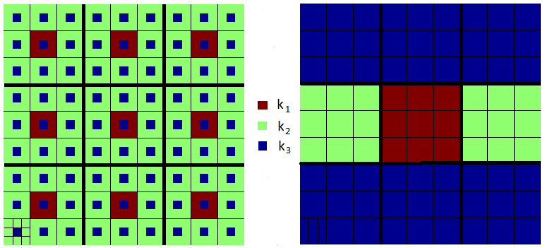
Figure 3: The setup for the two experiments with variations in coefficients $k_{1}$, $k_{2}$ and $k_{3}$. In both cases we have used the four-level method with $H^{\ell}/H^{\ell-1}=3$. The pictures show three levels of decomposition into subdomains with the first level decomposition shown only for one level $2$ subdomain, and the level of finite elements is not shown. The picture on the left shows the case when the coefficient variations are “interior” to the substructures on the top level, and the jumps in coefficients are aligned with the boundaries of substructures on lower levels. The picture on the right shows the case when the jumps in coefficients are aligned with the top level subdomain boundaries, and there are no “interior” variations.

In the second set of experiments, we have used the $\rho-$scaling and experimented with jumps in the coefficient$~{}k$. In particular we have performed two sets of experiments, both with the four level method and with $H^{\ell}/H^{\ell-1}=3$, $\ell=0,\dots,3$, see Figure 3. In the first experiment, the coefficient variations were “interior” to the substructures on the top level, and the jumps in coefficients were aligned with the substructure boundaries on lower levels. In the second experiment, the jumps in coefficients were aligned with the top level subdomain boundaries, and there were no “interior” coefficient variations. In both experiments we have kept the coefficient $k_{2}$ fixed as $k_{2}=1$, and varied $k_{1}$ up to $10^{2}$ and $k_{3}$ to as low as $10^{-2}$ in order to obtain a coefficient jump of maximum order$~{}10^{4}$. The iteration counts in all cases were nearly the same (with $2-3$ additional iterations) compared to those in Table 1. The results thus indicate that the convergence is independent of such jumps, which is also consistent (for the second setup) with the observations of Tu Tu-2011-TBA for the three-level BDDC method.

It thus appears that the Nested BDDC method can be also used for problems with variations of coefficients over multiple scales, if one is able to perform a somewhat special partitioning into subdomains. However, because we feel that this prevents a practical use of the proposed method for a realistic simulations with coefficient variations that might not be exactly aligned with the subdomain boundaries, we will address this issue in a separate study.

Table 1: The number of PCG iterations of the Multilevel BDDC preconditioner from Algorithm 5.1 for different relative subdomain sizes $H^{\ell}/H^{\ell-1}$, and different number of decomposition levels $L$ which determines the number of iterations of the Nested BDDC from Algorithm 5.2. For each decomposition level $\ell=1,\dots,L-1$, nsub is the number of subdomains, $n$ is the total number of degrees of freedom, $n_{\Gamma}$ is the number of degrees of freedom on the interfaces, iter is the number of PCG iterations with the $M$-level BDDC preconditioner where $M=L-\ell+1$. The stopping tolerance is $10^{-6}$, and cond is the condition number estimate from the Lánczos sequence in conjugate gradients.

$L$	$\ell$	$M$	nsub	$n$	$n_{\Gamma}$	iter	cond
$H_{\ell}/H_{\ell-1}=3$
2	1	2	9	261	36	4	1.22
3	2	2	9	225	36	3	1.14
	1	3	81	2241	432	8	2.07
4	3	2	9	225	36	3	1.14
	2	3	81	2133	432	7	1.84
	1	4	729	19,845	4212	11	3.48
5	4	2	9	225	36	3	1.14
	3	3	81	2133	432	7	1.83
	2	4	729	19,521	4212	10	3.09
	1	5	6561	177,633	38,880	14	5.98
$H_{\ell}/H_{\ell-1}=4$
2	1	2	16	800	96	6	1.94
3	2	2	16	736	96	5	1.73
	1	3	256	12,416	1920	10	3.45
4	3	2	16	736	96	5	1.72
	2	3	256	12,160	1920	9	3.11
	1	4	4096	197,120	32,256	14	6.62
$H_{\ell}/H_{\ell-1}=6$
2	1	2	36	3960	360	9	2.57
3	2	2	36	3816	360	9	2.30
	1	3	1296	140,400	15,120	13	5.60
$H_{\ell}/H_{\ell-1}=8$
2	1	2	64	12,416	896	10	3.00
3	2	2	64	12,160	896	10	2.72
	1	3	4096	787,456	64,512	17	7.46
$H_{\ell}/H_{\ell-1}=16$
2	1	2	256	197,120	7680	13	4.09
$H_{\ell}/H_{\ell-1}=32$
2	1	2	1024	3,147,776	63,488	15	5.25

References

• (1) Brenner, S.C., Sung, L.Y.: BDDC and FETI-DP without matrices or vectors. Comput. Methods Appl. Mech. Engrg. 196(8), 1429–1435 (2007)
• (2) Brezzi, F., Fortin, M.: Mixed and Hybrid Finite Element Methods. Springer-Verlag, New York – Berlin – Heidelberg (1991)
• (3) Cowsar, L.C., Mandel, J., Wheeler, M.F.: Balancing domain decomposition for mixed finite elements. Math. Comp. 64(211), 989–1015 (1995)
• (4) Cros, J.M.: A preconditioner for the Schur complement domain decomposition method. In: I. Herrera, D.E. Keyes, O.B. Widlund (eds.) Domain Decomposition Methods in Science and Engineering, pp. 373–380. National Autonomous University of Mexico (UNAM), México (2003). 14th International Conference on Domain Decomposition Methods, Cocoyoc, Mexico, January 6–12, 2002
• (5) Dohrmann, C.R.: A preconditioner for substructuring based on constrained energy minimization. SIAM J. Sci. Comput. 25(1), 246–258 (2003)
• (6) Ewing, R.E., Wang, J.: Analysis of the Schwarz algorithm for mixed finite element methods. RAIRO Mathematical Modelling and Numerical Analysis 26(6), 739–756 (1992)
• (7) Farhat, C., Lesoinne, M., Le Tallec, P., Pierson, K., Rixen, D.: FETI-DP: a dual-primal unified FETI method. I. A faster alternative to the two-level FETI method. Internat. J. Numer. Methods Engrg. 50(7), 1523–1544 (2001)
• (8) Farhat, C., Lesoinne, M., Pierson, K.: A scalable dual-primal domain decomposition method. Numer. Linear Algebra Appl. 7, 687–714 (2000)
• (9) Farhat, C., Roux, F.X.: A method of finite element tearing and interconnecting and its parallel solution algorithm. Internat. J. Numer. Methods Engrg. 32, 1205–1227 (1991)
• (10) Fragakis, Y., Papadrakakis, M.: The mosaic of high performance domain decomposition methods for structural mechanics: Formulation, interrelation and numerical efficiency of primal and dual methods. Comput. Methods Appl. Mech. Engrg. 192, 3799–3830 (2003)
• (11) Glowinski, R., Wheeler, M.F.: Domain decomposition and mixed finite element methods for elliptic problems. In: R. Glowinski, G.H. Golub, G.A. Meurant, J. Périaux (eds.) First International Symposium on Domain Decomposition Methods for Partial Differential Equations. SIAM, Philadelphia, PA (1988)
• (12) Klawonn, A., Rheinbach, O.: A hybrid approach to 3-level FETI. PAMM 8(1), 10,841–10,843 (2008). DOI 10.1002/pamm.200810841. 79th Annual Meeting of the International Association of Applied Mathematics and Mechanics (GAMM), Bremen 2008
• (13) Klawonn, A., Rheinbach, O., Widlund, O.B.: An analysis of a FETI-DP algorithm on irregular subdomains in the plane. SIAM J. Numer. Anal. 46(5), 2484–2504 (2008)
• (14) Li, J., Widlund, O.B.: BDDC algorithms for incompressible Stokes equations. SIAM J. Numer. Anal. 44(6), 2432–2455 (2006)
• (15) Li, J., Widlund, O.B.: FETI-DP, BDDC, and block Cholesky methods. Internat. J. Numer. Methods Engrg. 66(2), 250–271 (2006)
• (16) Mandel, J.: Balancing domain decomposition. Comm. Numer. Methods Engrg. 9(3), 233–241 (1993)
• (17) Mandel, J., Dohrmann, C.R., Tezaur, R.: An algebraic theory for primal and dual substructuring methods by constraints. Appl. Numer. Math. 54(2), 167–193 (2005)
• (18) Mandel, J., Sousedík, B.: Adaptive selection of face coarse degrees of freedom in the BDDC and the FETI-DP iterative substructuring methods. Comput. Methods Appl. Mech. Engrg. 196(8), 1389–1399 (2007)
• (19) Mandel, J., Sousedík, B.: BDDC and FETI-DP under minimalist assumptions. Computing 81, 269–280 (2007)
• (20) Mandel, J., Sousedík, B., Dohrmann, C.R.: Multispace and multilevel BDDC. Computing 83(2-3), 55–85 (2008)
• (21) Mathew, T.P.: Schwarz alternating and iterative refinement methods for mixed formulations of elliptic problems, part I: Algorithms and numerical results. Numer. Math. 65(4), 445–468 (1993)
• (22) Pavarino, L.F., Widlund, O.B.: Balancing Neumann-Neumann methods for incompressible Stokes equations. Comm. Pure Appl. Math. 55(3), 302–335 (2002)
• (23) Šístek, J., Sousedík, B., Burda, P., Mandel, J., Novotný, J.: Application of the parallel BDDC preconditioner to the Stokes flow. Comput. & Fluids 46, 429–435 (2011)
• (24) Sousedík, B.: Comparison of some domain decomposition methods. Ph.D. thesis, Czech Technical University in Prague, Faculty of Civil Engineering, Department of Mathematics (2008). http://mat.fsv.cvut.cz/doktorandi/files/BSthesisCZ.pdf
• (25) Sousedík, B.: Adaptive-Multilevel BDDC. Ph.D. thesis, University of Colorado Denver, Department of Mathematical and Statistical Sciences (2010). http://www.ucdenver.edu/academics/colleges/CLAS/Departments/math/students/alumni/Documents/Student%20Theses/Sousedik_Thesis.pdf
• (26) Sousedík, B., Mandel, J.: On Adaptive-Multilevel BDDC. In: Y. Huang, R. Kornhuber, O. Widlund, J. Xu (eds.) Domain Decomposition Methods in Science and Engineering XIX, Lecture Notes in Computational Science and Engineering 78, Part 1, pp. 39–50. Springer-Verlag (2011)
• (27) Toselli, A., Widlund, O.B.: Domain Decomposition Methods—Algorithms and Theory, Springer Series in Computational Mathematics, vol. 34. Springer-Verlag, Berlin (2005)
• (28) Tu, X.: A BDDC algorithm for mixed formulation of flow in porous media. Electron. Trans. Numer. Anal. 20, 164–179 (2005)
• (29) Tu, X.: BDDC domain decomposition algorithms: Methods with three levels and for flow in porous media. Ph.D. thesis, Department of Mathematics, New York University (2006). http://cs.nyu.edu/csweb/Research/TechReports/TR2005-879/TR2005-879.pdf
• (30) Tu, X.: A BDDC algorithm for flow in porous media with a hybrid finite element discretization. Electron. Trans. Numer. Anal. 26, 146–160 (2007)
• (31) Tu, X.: Three-level BDDC in three dimensions. SIAM J. Sci. Comput. 29(4), 1759–1780 (2007)
• (32) Tu, X.: Three-level BDDC in two dimensions. Internat. J. Numer. Methods Engrg. 69(1), 33–59 (2007)
• (33) Tu, X.: A three-level BDDC algorithm for a saddle point problem. Numerische Mathematik 119(1), 189–217 (2011)