The Variational Garrote

Abstract

In this paper, we present a new variational method for sparse regression using $L_{0}$ regularization. The variational parameters appear in the approximate model in a way that is similar to Breiman’s Garrote model. We refer to this method as the variational Garrote (VG). We show that the combination of the variational approximation and $L_{0}$ regularization has the effect of making the problem effectively of maximal rank even when the number of samples is small compared to the number of variables. The VG is compared numerically with the Lasso method, ridge regression and the recently introduced paired mean field method (PMF) titsias2012 . Numerical results show that the VG and PMF yield more accurate predictions and more accurately reconstruct the true model than the other methods. It is shown that the VG finds correct solutions when the Lasso solution is inconsistent due to large input correlations. Globally, VG is significantly faster than PMF and tends to perform better as the problems become denser and in problems with strongly correlated inputs. The naive implementation of the VG scales cubic with the number of features. By introducing Lagrange multipliers we obtain a dual formulation of the problem that scales cubic in the number of samples, but close to linear in the number of features.

1 Introduction

One of the most common problems in statistics is linear regression. Given $p$ samples of $n$-dimensional input data $x_{i}^{\mu},i=1,\ldots,n$ and 1-dimensional output data $y^{\mu}$, with $\mu=1,\ldots,p$, find weights $w_{i},w_{0}$ that best describe the relation

$$y^{\mu}=\sum_{i=1}^{n}w_{i}x_{i}^{\mu}+w_{0}+\xi^{\mu}$$ (1)

for all $\mu$. $\xi^{\mu}$ is zero-mean noise with inverse variance $\beta$.

The ordinary least square (OLS) solution is given by $\vec{w}=\chi^{-1}\vec{b}$ and $w_{0}=\bar{y}-\sum_{i}w_{i}\bar{x}_{i}$, where $\chi$ is the input covariance matrix $\vec{b}$ is the vector of input-output covariances and $\bar{x}_{i},\bar{y}$ are the mean values. There are several problems with the OLS approach. When $p$ is small, it typically has a low prediction accuracy due to over fitting. In particular, when $p<n$, $\chi$ is not of maximal rank and so its inverse is not uniquely defined. In addition, the OLS solution is not sparse: it will find a solution $w_{i}\neq 0$ for all $i$. Therefore, the interpretation of the OLS solution is often difficult.

These problems are well-known, and there exist a number of approaches to overcome these problems. The simplest approach is called ridge regression. It adds a regularization term $\frac{1}{2}\lambda\sum_{i}w_{i}^{2}$ with $\lambda>0$ to the OLS criterion. This has the effect that the input covariance matrix $\chi$ gets replaced by $\chi+\lambda I$ which is of maximal rank for all $p$. One optimizes $\lambda$ by cross validation. Ridge regression improves the prediction accuracy but not the interpretability of the solution.

Another approach is Lasso tibshirani96 . It solves the OLS problem under the linear constraint $\sum_{i}|w_{i}|\leq t$. This problem is equivalent to adding an $L_{1}$ regularization term $\lambda\sum_{i}|w_{i}|$ to the OLS criterion. The optimization of the quadratic error under linear constraints can be solved efficiently. See friedman2009 for a recent account. Again, $\lambda$ or $t$ may be found through cross validation. The advantage of the $L_{1}$ regularization is that the solution tends to be sparse. This improves both the prediction accuracy and the interpretability of the solution.

The $L_{1}$ or $L_{2}$ regularization terms are known as shrinkage priors because their effect is to shrink the size of $w_{i}$. The idea of shrinkage prior has been generalized by frank1993 to the form $\lambda\sum_{i}|w_{i}|^{q}$ with $q>0$ and $q=1,2$ corresponding to the Lasso and ridge case, respectively. Better solutions can be obtained for $q<1$, however the resulting optimization problem is no longer convex and therefore more difficult to solve.

An alternative Bayesian approach to obtain a sparse solution using an $L_{0}$ penalty was proposed by george1993 . They introduce $n$ variational selector variables $s_{i}$ such that the prior distribution over $w_{i}$ is a mixture of a narrow (spike) and wide (slab) Gaussian distribution, both centered on zero. The posterior distribution over $s_{i}$ indicates whether the input feature $i$ is included in the model or not. Since the number of subsets of features is exponential in $n$, for large $n$ one cannot compute the solution exactly. In addition, the posterior is a complex high dimensional distribution of the $w_{i}$ and the other (hyper) parameters of the model. The computation of the posterior requires thus the use of MCMC sampling george1993 or a variational Bayesian approximation titsias2012 ; logsdon2010 ; Yoshida ; lobato .

Although Bayesian approaches tend to over fit less than a maximum likelihood or maximum a posteriori method (MAP approach), they also tend to be relatively slow. Here we propose a partial Bayesian approach, where we apply a variational approximation to integrate out the binary (selector) variables in combination with a MAP approach for the remaining parameters. For clarity, we analyse this idea in its most simple form, in the absence of (hierarchical) priors. Instead, we infer the sparsity prior through cross validation. As we will motivate below, we call the method the Variational Garrote (VG).

The paper is organized as follows. In section 2 we introduce the model and we derive the variational approximation. We show that the combination of the variational approximation and $L_{0}$ regularization has the effect of making the problem effectively of maximal rank by introducing a ’variational ridge term’. As a result, the solution is well defined even when $p<n$ as long as the number of predictive features is less than $p$ (which is controlled by the sparsity prior).

To gain further insight, in section 3 we study the case when the design matrix is orthogonal. In this case the solution can be computed exactly in closed form with no need to resort to approximations. In the variational approximation, we show for the uni-variate case that the solution is either unique or has two solutions, depending on the input-output correlations, the number of samples $p$ and on the sparsity prior $\gamma$. We derive a phase plot and show that the solution is unique, when the sparsity prior is not too strong or when the input-output correlation is not too large. The input-output behavior of the VG is shown to be close to optimal as a smoothed version of hard feature selection. We argue that this behavior also holds in the multi-variate case.

In section 4 we compare the VG with a number of other MAP methods, such as Lasso and ridge regression and with the paired mean field method (PMF) titsias2012 , a recently proposed variational bayesian method. We show that the VG and PMF significantly outperform the Lasso and ridge regression on a large number of different examples both in terms of the accuracy of the solution, as well as in prediction error. In addition, we show that the VG do not suffer from the inconsistency of the Lasso method when the input correlations are large. We show in detail how all methods compare as a function of the level of noise, the sparsity of the target solution, the number of samples and the number of irrelevant predictors. Globally, VG is significantly faster than PMF and tends to perform better as the problems become denser and in problems with strongly correlated inputs.

2 The variational approximation

Consider the regression model of the form

$$y^{\mu}=\sum_{i=1}^{n}w_{i}s_{i}x^{\mu}_{i}+\xi^{\mu}\qquad\sum_{i=1}^{n}s_{i}\leq t$$ (2)

with $s_{i}=0,1$. The bits $s_{i}=1$ will identify the predictive inputs $i$. Using a Bayesian description, and denoting the data by $D:\{\vec{x}^{\mu},y^{\mu}\},\mu=1,\ldots,p$, the likelihood term is given by

$$p(y|\vec{x},\vec{s},\vec{w},\beta) =\sqrt{\frac{\beta}{2\pi}}\exp\left(-\frac{\beta}{2}\left(y-\sum_{i=1}^{n}w_{i}s_{i}x_{i}\right)^{2}\right)$$

$$p(D|\vec{s},\vec{w},\beta) =\prod_{\mu}p(y^{\mu}|\vec{x}^{\mu},\vec{s},\vec{w},\beta)$$

$$=\left(\frac{\beta}{2\pi}\right)^{p/2}\exp\left(-\frac{\beta p}{2}\left(\sum_{i,j=1}^{n}s_{i}s_{j}w_{i}w_{j}\chi_{ij}-2\sum_{i=1}^{n}w_{i}s_{i}b_{i}+\sigma_{y}^{2}\right)\right)$$ (3)

with $b_{i}=\frac{1}{p}\sum_{\mu}x_{i}^{\mu}y^{\mu},\sigma_{y}^{2}=\frac{1}{p}\sum_{\mu}(y^{\mu})^{2},\chi_{ij}=\frac{1}{p}\sum_{\mu}x_{i}^{\mu}x_{j}^{\mu}$.

We should also specify prior distributions over $\vec{s},\vec{w},\beta$. For concreteness, we assume that the prior over $\vec{s}$ is factorized over the individual $s_{i}$, each with identical prior probability:

$$p(\vec{s}|\gamma) =\prod_{i=1}^{n}p(s_{i}|\gamma) p(s_{i}|\gamma) =\frac{\exp\left(\gamma s_{i}\right)}{1+\exp(\gamma)}$$ (4)

with $\gamma$ given which specifies the sparsity of the solution. We denote by $p(\vec{w},\beta)$ the prior over the inverse noise variance $\beta$ and the feature weights $\vec{w}$. We will leave this prior unspecified since its choice does not affect the variational approximation.

The posterior becomes

$$p(\vec{s},\vec{w},\beta|D,\gamma)=\frac{p(\vec{w},\beta)p(\vec{s}|\gamma)p(D|\vec{s},\vec{w},\beta)}{p(D|\gamma)}$$ (5)

Computing the MAP estimate or computing statistics from the posterior is complex in particular due to the discrete nature or $\vec{s}$. We propose to compute a variational approximation to the marginal posterior $p(\vec{w},\beta|D,\gamma)=\sum_{\vec{s}}p(\vec{s},\vec{w},\beta|D,\gamma)$ and computing the MAP solution with respect to $\vec{w},\beta$. Since $p(D|\gamma)$ does not depend on $\vec{w},\beta$ we can ignore it.

The posterior distribution Eq. 5 for given $\vec{w},\beta$ is a typical Boltzmann distribution involving terms linear and quadratic in $s_{i}$. It is well-known that when the effective couplings $w_{i}w_{j}\chi_{ij}$ are small, one can obtain good approximations using methods that originated in the statistical physics community and where $s_{i}$ denote binary spins. Most prominently, one can use the mean field or variational approximation jordan1998 , the TAP approximation kap99e or belief propagation (BP) murphy99 . For introductions into these methods also see opper2001a ; wainwright2008 . Here, we will develop a solution based on the simplest possible variational approximation and leave the possible improvements using BP or structured mean field approximations to the future.

We approximate the sum by the variational bound using Jensen’s inequality.

$$\log\sum_{\vec{s}}p(\vec{s}|\gamma)p(D|\vec{s},\vec{w},\beta) \geq-\sum_{\vec{s}}q(\vec{s})\log\frac{q(\vec{s})}{p(\vec{s}|\gamma)p(D|\vec{s},\vec{w},\beta)}$$

$$=-F(q,\vec{w},\beta)$$ (6)

$q(\vec{s})$ is called the variational approximation and can be any positive probability distribution on $\vec{s}$ and $F(q,\vec{w},\beta)$ is called the variational free energy. The optimal $q(\vec{s})$ is found by minimizing $F(q,\vec{w},\beta)$ with respect to $q(\vec{s})$ so that the tightest bound - best approximation - is obtained.

In order to be able to compute the variational free energy efficiently, $q(\vec{s})$ must be a tractable probability distribution, such as a chain or a tree with limited tree-width barber98b . Here we consider the simplest case where $q(\vec{s})$ is a fully factorized distribution: $q(\vec{s})=\prod_{i=1}^{n}q_{i}(s_{i})$ with $q_{i}(s_{i})=m_{i}s_{i}+(1-m_{i})(1-s_{i})$, so that $q$ is fully specified by the expected values $m_{i}=q_{i}(s_{i}=1)$, which we collectively denote by $\vec{m}$. The expectation values with respect to $q$ can now be easily evaluated and the result is

$$F =\frac{\beta p}{2}\left(\sum_{i,j}^{n}m_{i}m_{j}w_{i}w_{j}\chi_{ij}+\sum_{i}m_{i}(1-m_{i})w_{i}^{2}\chi_{ii}-2\sum_{i=1}^{n}m_{i}w_{i}b_{i}+\sigma_{y}^{2}\right)$$

$$-\gamma\sum_{i=1}^{n}m_{i}+\sum_{i=1}^{n}\left(m_{i}\log m_{i}+(1-m_{i})\log(1-m_{i})\right)-\frac{p}{2}\log\frac{\beta}{2\pi}$$ (7)

where we have omitted terms independent of $m,\beta,w$. The first line is due to the likelihood term, the second line is due to the prior on $\vec{s}$ and the entropy of $q(\vec{s})$. The approximate marginal posterior is then

$$p(\vec{w},\beta|D,\gamma) \propto p(\vec{w},\beta)\sum_{\vec{s}}p(\vec{s}|\gamma)p(D|\vec{s},\vec{w},\beta)$$

$$\approx p(\vec{w},\beta)\exp(-F(\vec{m},\vec{w},\beta,\gamma))$$

We can compute the variational approximation $\vec{m}$ for given $\vec{w},\beta,\gamma$ by minimizing $F$ with respect to $\vec{m}$. In addition, $p(\vec{w},\beta|D,\gamma)$ needs to be maximized with respect to $\vec{w},\beta$. Note, that the variational approximation only depends on the likelihood term and the prior on $\gamma$, since these are the only terms that depend on $\vec{s}$. Thus, for given $\vec{w}$, the variational approximation does not depend on the particular choices for the prior $p(\vec{w},\beta)$. For concreteness, we assume a flat prior $p(\vec{w},\beta)\propto 1$. We set the derivatives of $F$ with respect $\vec{m},\vec{w},\beta$ equal to zero. This gives the following set of fixed point equations:

$$m_{i} = \sigma\left(\gamma+\frac{\beta p}{2}w_{i}^{2}\chi_{ii}\right)$$ (8)

$$\vec{w} = (\chi^{\prime})^{-1}\vec{b}\qquad\chi^{\prime}_{ij}=\chi_{ij}m_{j}+(1-m_{j})\chi_{jj}\delta_{ij}$$ (9)

$$\frac{1}{\beta} = \sigma_{y}^{2}-\sum_{i=1}^{n}m_{i}w_{i}b_{i}$$ (10)

with $\sigma(x)=(1+\exp(-x))^{-1}$ and where in Eq. 10 we have used Eq. 9. Eqs. 8-10 provide the final solution. They can be solved by fixed point iteration as outlined in Algorithm 1: Initialize $\vec{m}$ at random. Compute $\vec{w}$ by solving the linear system Eq. 9 and $\beta$ from Eq. 10. Compute a new solution for $\vec{m}$ from Eq.8.

Within the variational/MAP approximation the predictive model is given by

$$y = \sum_{i}m_{i}w_{i}x_{i}+\xi$$ (11)

with $\left<\xi^{2}\right>=1/\beta$ and $\vec{m},\vec{w},\beta$ as estimated by the above procedure. Eq. 11 has some similarity with Breiman’s non-negative Garrote method breiman93 . It computes the solution in a two step approach: it computes first $w_{i}$ using OLS and then finds $m_{i}$ by minimizing

$$\sum_{\mu}\left(y^{\mu}-\sum_{i=1}^{n}x_{i}^{\mu}w_{i}m_{i}\right)^{2}\quad\mathrm{subject~{}to}\quad m_{i}\geq 0\quad\sum_{i}m_{i}\leq t$$

Because of this similarity, we refer to our method as the variational Garrote (VG). Note, that because of the OLS step the non-negative garrote requires that $p\geq n$. Instead, the variational solution Eqs. 8-10 computes the entire solution in one step (and as we will see does not require $p\geq n$).

Let us pause to make some observations about this solution. One might naively expect that the variational approximation would simply consist of replacing $w_{i}s_{i}$ in Eq. 2 by its variational expectation $w_{i}m_{i}$. If this were the case, $\vec{m}$ would disappear entirely from the equations and one would expect in Eq. 9 the OLS solution with the normal input covariance matrix $\chi$ instead of the new matrix $\chi^{\prime}$ (note, that in the special case that $m_{i}=1$ for all $i$, $\chi^{\prime}=\chi$ and Eq. 9 does reduce to the OLS solution). Instead, $\vec{m}$ and $\vec{w}$ are both to be optimized, giving in general a different solution than the OLS solution .

When $m_{i}<1$, $\chi^{\prime}$ differs from $\chi$ by rescaling with $m_{i}$ and adding a positive diagonal to it, a ’variational ridge’. This is similar to the mechanism of ridge regression, but with the important difference that the diagonal term depends on $i$ and is dynamically adjusted depending on the solution for $\vec{m}$. Thus, the sparsity prior together with variational approximation provides a mechanism that solves the rank problem. When all $m_{i}<1$, $\chi^{\prime}$ is of maximal rank. Each $m_{i}$ that approaches 1, reduces the rank by one. Thus, if $\chi$ has rank $p<n$, $\chi^{\prime}$ can be still of rank $n$ when no more than $p$ of the $m_{i}=1$, the remaining $n-p$ of the $m_{i}<1$ making up for the rank deficiency. Note, that the size of $m_{i}$ (and thus the rank of $\chi^{\prime}$) is controlled by $\gamma$ through Eq. 8.

In the above procedure, we compute the VG solution for fixed $\gamma$ and choose its optimal value through cross validation on independent data mitchell1988 . This has the advantage that our result is independent of our (possibly incorrect) prior belief.

But another important advantage of varying $\gamma$ manually is that it helps to avoid local minima. When we increase $\gamma$ from a negative value $\gamma_{\mathrm{min}}$ to a maximal value $\gamma_{\mathrm{max}}$ in small steps, we obtain a sequence of solutions with decreasing sparseness. These solutions will better fit the data and as a result $\beta$ increases with $\gamma$. Thus, increasing $\gamma$ implements an annealing mechanism where we sequentially obtain solutions at lower noise levels. We found empirically that this approach is effective to reduce the problem of local minima. To further deal with the effect of hysteresis (see section 3) we recompute the solution from $\gamma_{\mathrm{max}}$ down to $\gamma_{\mathrm{min}}$ and choose the solution with lowest free energy.

The minimal value of $\gamma$ is chosen as the largest value such that $m_{i}=\epsilon$, with $\epsilon$ small. We find from Eqs. 8-10 that

$$\gamma_{\mathrm{min}}=-\frac{pb_{i}^{2}\chi_{ii}}{2\sigma_{y}^{2}}+\sigma^{-1}(\epsilon)+{\cal O}(\epsilon)$$ (12)

with $\sigma^{-1}(x)=\log(x/(1-x))$. We heuristically set the maximal value of $\gamma$ as well as the step size.

In appendix B we provide an alternative fixed point iteration scheme that is more efficient in the large $n$ small $p$ limit. Whereas Eqs. 8-10 require the repeated solution of a $n$-dimensional linear system, the dual formulation, Eqs. (8),(21),(24)-(27), requires the repeated solution of a $p$ dimensional linear system. Algorithm 1 summarizes the VG method.

input : Data $D:\{\vec{x}^{\mu},y^{\mu}\},\mu=1,\ldots,p$ ; $\epsilon$ and step-size $\Delta\gamma$

output : $\vec{w},\vec{m},\beta,\gamma$ solution with minimal cross validation error

1 Preprocess data such that $\sum_{\mu}x_{i}^{\mu}=\sum_{\mu}y^{\mu}=0$ and partition $D$ in $D^{\text{train}}$, $D^{\text{val}}$

2 Compute $b_{i}=\frac{1}{p}\sum_{\mu}x_{i}^{\mu}y^{\mu}$ and if $n<p$ compute $\chi_{ij}=\frac{1}{p}\sum_{\mu}x_{i}^{\mu}x_{j}^{\mu}$

3 Compute $\gamma_{\mathrm{min}}$ from $\epsilon$ and $\gamma_{\mathrm{max}}$ from $\gamma_{\mathrm{min}}$ and $\Delta\gamma$

4 for $\gamma=\gamma_{\mathrm{min}}:\Delta\gamma:\gamma_{\mathrm{max}}$ do // FORWARD PASS

      5 $\eta\leftarrow 1$

      6 while not converged do

            7 Compute $\vec{w},\beta$ from Eqs. (9)-(10) ($n<p$) or Eqs. (21), (24)-(27) ($n>p$);

            8Compute $\vec{m}^{\prime}$ using a smoothed version of Eq. (8): $m_{i}^{\prime}\leftarrow(1-\eta)m_{i}+\eta\sigma(\ldots)$

            9 if $\max_{i}|m_{i}^{\prime}-m_{i}|>0.1$ then

                  10 $\eta\leftarrow\eta/2$

            11 $\vec{m}\leftarrow\vec{m}^{\prime}$

            

      12 Store solution $(\vec{w}_{1},\vec{m}_{1},\beta_{1})_{\gamma}$ and $F_{1}(\gamma)\leftarrow F((\vec{w}_{1},\vec{m}_{1},\beta_{1})_{\gamma})$ from Eq. (2)

      

13 for $\gamma=\gamma_{\mathrm{max}}:-\Delta\gamma:\gamma_{\mathrm{min}}$ do // BACKWARD PASS

      14 As $\mathbf{5}-\mathbf{11}$

      15 Store solution $(\vec{w}_{2},\vec{m}_{2},\beta_{2})_{\gamma}$ and $F_{2}(\gamma)\leftarrow F((\vec{w}_{2},\vec{m}_{2},\beta_{2})_{\gamma})$ from Eq. (2)

      

16 for $\gamma=\gamma_{\mathrm{min}}:\Delta\gamma:\gamma_{\mathrm{max}}$ do

      17 Choose solution $(\vec{w},\vec{m},\beta)_{\gamma}$ that has minimal $F_{1,2}(\gamma)$

      18 Compute cross validation error on $D^{\text{val}}$ using Eq. (11)

      

19 Select $\vec{w},\vec{m},\beta,\gamma$ with minimal cross validation error

Algorithm 1 The Variational Garrote algorithm.

3 Orthogonal and uni-variate case

In order to obtain further insight in the solution, consider the case in which the inputs are uncorrelated: $\chi_{ij}=\delta_{ij}$. In this case, we can derive the MAP solution of Eq. 5 exactly, without the need to resort to the variational approximation. Eq. 5 reduces to a distribution that factorizes over $i$ with log probability proportional to

$$L=\frac{p}{2}\log\beta-\frac{\beta p}{2}\left(\sum_{i=1}^{n}s_{i}(w_{i}^{2}-2w_{i}b_{i})+\sigma_{y}^{2}\right)+\gamma\sum_{i=1}^{n}s_{i}$$

Maximizing wrt $w_{i},\beta$ yields $w_{i}=b_{i}$, $\beta^{-1}=\sigma_{y}^{2}-\sum_{i=1}^{n}s_{i}b_{i}^{2}$ and

$$L=\frac{p}{2}\log\beta+\sum_{i=1}^{n}s_{i}\left(\frac{\beta p}{2}b_{i}^{2}+\gamma\right)-\frac{\beta p}{2}\sigma_{y}^{2}$$

Assume without loss of generality that $b_{i}^{2}$ are sorted in decreasing order. $L$ is maximized by setting $s_{i}=1$ when $\frac{\beta p}{2}b_{i}^{2}+\gamma>0$ and $s_{i}=0$ otherwise. Thus, the optimal solution is $s_{1:k}=1,s_{k+1:n}=0$, $\beta^{-1}=\sigma_{y}^{2}-\sum_{i=1}^{k}b_{i}^{2}$ with $k$ the smallest integer such that

$$\frac{\beta p}{2}b_{k+1}^{2}+\gamma<0$$ (13)

By varying $\gamma$ from small to large, we find a sequence of solutions with decreasing sparsity.

In the variational approximation the solution is very similar but not identical. Eq. 9 gives the same solution $w_{i}=b_{i}$. Eqs. 8 and 10 become

$$m_{i} = \sigma\left(\gamma+\frac{\beta p}{2}b_{i}^{2}\right)$$

$$1/\beta = \sigma_{y}^{2}-\sum_{i}b_{i}^{2}m_{i}$$

which we can interpret as the variational approximations of Eq. 13, with $m_{1:k}\approx 1$ and $m_{k+1:n}\approx 0$. The term $\sum_{i}b_{i}^{2}m_{i}$ is the explained variance and is subtracted from the total output variance to give an estimate of the noise variance $1/\beta$.

Note that the posterior is factorized in $s_{i}$, the variational approximation is not identical to the exact map solution Eq. 13, although the results are very similar. The relation is $s_{i}=0\Leftrightarrow m_{i}<0.5$ and $s_{i}=1\Leftrightarrow m_{i}>0.5$.

In order to further analyze the variational solution, we consider the $1$-dimensional case. The variational equations become

$$m = \sigma\left(\gamma+\frac{p}{2}\frac{\rho}{1-\rho m}\right)=f(m)$$ (14)

$$\frac{1}{\beta} = \sigma^{2}_{y}(1-m\rho)$$ (15)

with $\rho=b^{2}/\sigma_{y}^{2}$ the squared correlation coefficient.

In Eq. 14, we have eliminated $\beta$ and we must find a solution for $m$ for this non-linear equation. We see that it depends on the input-output correlation $\rho$, the number of samples $p$ and the sparsity $\gamma$. For $p=100$, the solution for different $\rho,\gamma$ is illustrated in figure 10 (see appendix A).

Figure 1: Phase plot $\rho,\gamma$ for $p=100$ giving the different solutions for $m$. Dashed and dot-dashed lines for $\rho>\rho^{*}=0.28$ are from Eq. 18 where two solutions for $m$ exist. Solid line for $\rho<\rho^{*}$ is the solution for $\gamma$ when $m=1/2$, to indicate the transition from the unique solution $m\approx 0$ to the unique solution $m\approx 1$. Dotted line is the exact transition from $s=0$ to $s=1$ from Eq. 13. Insets indicate solutions for $m$ versus $\rho$ for $\gamma=-10,p=100$ (top-right) and for $\gamma=-40,p=100$ (bottom-left). In the lower left corner of the insets, the unique solution $m\approx 0$ is found. In the top right corner, the unique solution $m\approx 1$ is found. Between the dot-dashed and the dashed line, the two variational solutions $m\approx 0$ and $m\approx 1$ co-exist.

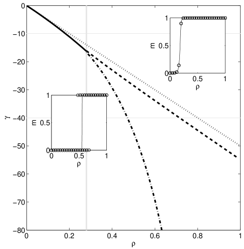
Eq. 14 has one or three solutions for $m$, depending on the values of $\gamma,\rho,p$. The three solutions correspond to two local minima and one local maximum of the free energy $F$. For $\gamma=-40$ and $\gamma=-10$, we plot the stable solution(s) for different values of $\rho$ in the inserts in fig. 1. The best variational solution for $m$ is given by the solution with the lowest free energy, indicated by the solid lines in the inserts in fig. 1.

Fig. 1 further shows the phase plot of $\gamma,\rho$ that indicates that the variational solution is unique for $\gamma>\gamma^{*}$ or for $\rho<\rho^{*}$. The solid line for $0<\rho<\rho^{*}$ in fig. 1 indicates a smooth (second order) phase transition from $m=0$ to $m=1$. For $\rho>\rho^{*}$, the transition from $m=0$ to $m=1$ is discontinuous: for each $\rho$ there is a range of values of $\gamma$ where two variational solutions $m\approx 0$ and $m\approx 1$ co-exist. For comparison, we also show the line $\gamma=-p\rho/2$ that separates the solution $s=0$ and $s=1$ according the the exact (non-variational) solution Eq. 13.

The multi-valued variational solution results in a hysteresis effect. When the solution is computed for increasing $\gamma$, the $m\approx 0$ solution is obtained until it no longer exists. If the sequence of solutions is computed for decreasing $\gamma$ the $m\approx 1$ solution is obtained for values of $\gamma$ where previously the $m\approx 0$ solution was obtained.

From this simple one-dimensional case we may infer that the variational approximation is relatively easy to compute in the uni-modal region (small $\rho$ or $\gamma$ not too negative) and becomes more inaccurate in the region where multiple minima exist (region between the dot-dashed and dashed lines in fig. 1) .

It is interesting to compare the uni-variate solution of the variational garrote with ridge regression, Lasso or Breiman’s Garrote, which was previously done for the latter three methods in tibshirani96 . Suppose that data are generated from the model $y=wx+\xi$ with $\left<\xi^{2}\right>=\left<x^{2}\right>=1$. We compare the solutions as a function of $w$. The OLS solution is approximately given by $w_{\mathrm{ols}}\approx\left<xy\right>=w$, where we ignore the statistical deviations of order $1/p$ due to the finite data set size. Similarly, the ridge regression solution is given by $w_{\mathrm{ridge}}\approx\lambda w$, with $0<\lambda<1$ depending on the ridge prior. The Lasso solution (for non-negative $w$) is given by $w_{\mathrm{lasso}}=(w-\gamma)^{+}$ tibshirani96 , with $\gamma$ depending on the $L_{1}$ constraint. Breiman’s Garrote solution is given by $w_{\mathrm{garrote}}=(1-\frac{\gamma}{w^{2}})^{+}w$ tibshirani96 , with $\gamma$ depending on the $L_{1}$ constraint. The VG solution is given by $w_{\mathrm{vg}}=mw$, with $m$ the solution of Eq. 14. Note, that the VG solution depends, in addition to $w,\gamma$, on the unexplained variance $\sigma_{y}^{2}$ and the number of samples $p$, whereas the other methods do not.

The qualitative difference of the solutions is shown in fig. 2.

Figure 2: Uni-variate solution for different regression methods. All methods yield a shrinked solution (deviation from diagonal line). Variational Garrote (VG) with $\gamma=-10,p=100$ and $\sigma_{y}^{2}=1$. Ridge regression with $\lambda=0.5$. Garrote with $\gamma=1/4$. Lasso with $\gamma=1/2$.

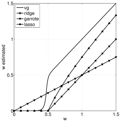
The ridge regression solution is off by a constant multiplicative factor. The Lasso solution is zero for small $w$ and for larger $w$ gives a solution that is shifted downwards by a constant factor. Breiman’s Garrote is identical to the Lasso for small $w$ and shrinks less for larger $w$. The VG gives an almost ideal behavior and can be interpreted as a soft version of variable selection: For small $w$ the solution is close to zero and the variable is ignored, and above a threshold it is identical to the OLS solution.

The qualitative nature of the phase plot fig. 1 and the input-output behavior fig. 2 extends to the multi-variate orthogonal case. The symmetry breaking of feature $i$ is independent of all other features, except for the term $\delta=\sum_{j\neq i}b_{j}^{2}m_{j}$ that enters through $\beta$. If we increase $\gamma$, $\delta$ increases in steps each time that one of the features $j$ switches from $m_{j}\approx 0$ to $m_{j}\approx 1$. Thus $\delta$ is constant almost always, except at the step points. Since the critical values of $\rho$ and $\gamma$ depend in a simple way on $\delta$, the phase plot for the multivariate orthogonal case is qualitatively the same as for the uni-variate case.

4 Numerical examples

In the following examples, we compare the VG with Lasso, ridge regression and in some cases, with the paired mean field approach (PMF) titsias2012 .

For most of the examples, we generate a training set, a validation set and a test set. Inputs are generated from a zero mean multi-variate Gaussian distribution with specified covariance structure. We generate outputs $y^{\mu}=\sum_{i}\hat{w}_{i}x_{i}^{\mu}+d\xi^{\mu}$ with $d\xi^{\mu}\in{\cal N}(0,\hat{\sigma})$ and $\hat{w}_{i}$ depending on the problem.

For VG, ridge regression and Lasso, we optimize the model parameters on the training set and, when necessary, optimize the hyper parameters ($\gamma$ in the case of VG, $\lambda$ in the case of ridge regression and Lasso) that minimize the quadratic error on the validation set. For the Lasso, we used the method described in friedman2009 .

Comparison with PMF is performed using the software available online for the regression case with one-dimensional output . Since PMF optimizes hyperparameters as well, we merge both training and validation sets and the resulting dataset is used as input for the PMF method. This ensures that all methods use the same data for parameter estimation.

We define the solution vector for a given method as $\vec{v}$. For VG, the components are $v_{i}\equiv m_{i}w_{i}$. In the case of PMF, $m_{i}$ corresponds to the spike-and-slab variational posterior and $w_{i}$ to the variational mean for the weights . For Ridge and Lasso $v_{i}\equiv w_{i}$.

4.1 Small Example 1

In the first example, we take independent inputs $x_{i}^{\mu}\in{\cal N}(0,1)$ and a teacher weight vector with only one non-zero entry: $\hat{w}=(1,0,\ldots,0)$, $n=100$ and $\hat{\sigma}=1$. The training set size $p=50$, validation set size $p_{v}=50$ and test set size $p_{t}=400$.

Figure 3: Top left (a): Minimal variational free energy versus $\gamma$. The two curves correspond to warm start solution from small to large $\gamma$ (’forward’) and from large to small $\gamma$ (’backward’) (see also Algorithm 1). Top right (b): Training and validation error versus $\gamma$. The optimal $\gamma$ minimizes the validation error. Bottom left (c): Solution $v_{1}=m_{1}w_{1}$ and $\max_{i=2:n}|m_{i}w_{i}|$. The correct solution is found in the range $\gamma\approx-20$ to $\gamma\approx-5$. Bottom right (d): Optimal solution $v_{i}=w_{i}m_{i}$ versus $i$.

We choose $\epsilon=0.001$ in Eq. 12, $\gamma_{\mathrm{max}}=0.02\gamma_{\mathrm{min}},\Delta\gamma=-0.02\gamma_{\mathrm{min}}$ (see Algorithm 1 for details).

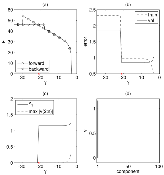
Results for a single run of the VG are shown in fig. 3. In fig. 3a, we plot the minimal variational free energy $F$ versus $\gamma$ for both the forward and backward run. Note, the hysteresis effect due to the local minima. For each $\gamma$, we use the solution with the lowest $F$. In fig. 3b, we plot the training error and validation error versus $\gamma$. The optimal $\gamma\approx-21$ is denoted by a star and the corresponding $\sigma=1/\sqrt{\beta}=1.05$. In fig. 3c, we plot the non-zero component $v_{1}=m_{1}w_{1}$ and the maximum absolute value of the remaining components versus $\gamma$. Note the robustness of the VG solution in the sense of the large range of $\gamma$ values for which the correct solution is found. In fig. 3d, we plot the optimal solution $v_{i}=m_{i}w_{i}$ versus $i$.

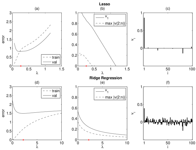
In fig. 4 we show the Lasso (top row) and ridge regression (bottom row) results for the same data set. The optimal value for $\lambda$ minimizes the validation error (star). In fig. 4b,c we see that the Lasso selects a number of incorrect features as well. Fig.  4b also shows that the Lasso solution with a larger $\lambda$ in the range $0.45<\lambda<0.95$ could select the single correct feature, but would then estimate $\hat{w}_{1}$ too small due to the large shrinkage effect. Ridge regression gives very bad results. The non-zero feature is too small and the remaining features have large values. Note from fig. 4e, that ridge regression yields a non-sparse solution for all values of $\lambda$.

Figure 4: Regression solution for Lasso and ridge regression for same data set as in fig. 3. Top row (a,b,c): Lasso. Bottom row (d,e,f): Ridge regression. Left column (a,d): training and validation errors versus $\lambda$. Middle column (b,e): Solution for the non-zero feature $v_{1}$ and the zero-features $\max_{i=2:n}|v_{i}|$. Right column (c,f): Optimal Lasso and ridge regression solution $v_{i}$ versus $i$.

	Train	Val	Test	# non-zero	$\|\delta\vec{v}\|_{1}$
Ridge	$0.60\pm 0.43$	$1.72\pm 0.39$	$1.80\pm 0.12$	$-$	$3.97\pm 1.23$
Lasso	$0.78\pm 0.26$	$1.07\pm 0.20$	$1.17\pm 0.20$	$8.65\pm 6.75$	$0.80\pm 0.57$
PMF	$-$	$-$	$1.02\pm 0.10$	$1.5\pm 1.19$	$0.33\pm 0.37$
VG	$0.85\pm 0.22$	$0.96\pm 0.17$	$1.01\pm 0.10$	$1.20\pm 0.52$	$0.31\pm 0.30$
True	$0.93\pm 0.14$	$0.87\pm 0.20$	$0.98\pm 0.04$	$1$	$0$

Table 1: Results for Example 1 averaged over 20 instances. Train is mean squared error (MSE) on the training set. Val is MSE on the validation set. Test is MSE on the test set. # non-zero is the number of non-zero elements in the Lasso solution and $\sum_{i=1}^{n}(m_{i}>0.5)$ for VG and PMF. $\|\delta\vec{v}\|_{1}=\sum_{i=1}^{n}|v_{i}-\hat{w}_{i}|$.

Table 1 shows that the VG significantly outperforms the Lasso method and ridge regression both in terms of prediction error, the accuracy of the estimation of the parameters and the number of non-zero parameters. In this simple example, there is no significant difference in the prediction error of Lasso, PMF and VG, but the Lasso solution is significantly less sparse. There is no significant difference between the solutions found by PMF and VG.

4.2 Small Example 2

In the second example, we consider the effect of correlations in the input distribution. Following tibshirani96 we generate input data from a multi-variate Gaussian distribution with covariance matrix $\chi_{ij}=\zeta^{|i-j|}$, with $\zeta=0.5$. In addition, we choose multiple features non-zero: $\hat{w}_{i}=1,i=1,2,5,10,50$ and all other $\hat{w}_{i}=0$. We use $n=100,\hat{\sigma}=1$ and $p/p_{v}/p_{t}=50/50/400$. In table 2 we compare the performance of the VG, Lasso, ridge regression and PMF on 20 random instances.

	Train	Val	Test	# non-zero	$\|\delta\vec{v}\|_{1}$
Ridge	$0.32\pm 0.27$	$3.30\pm 0.67$	$3.46\pm 0.31$	$-$	$11.09\pm 0.93$
Lasso	$0.75\pm 0.37$	$1.39\pm 0.37$	$1.48\pm 0.29$	$16.30\pm 6.60$	$2.08\pm 0.87$
PMF	$-$	$-$	$1.06\pm 0.11$	$5.15\pm 0.49$	$0.67\pm 0.35$
VG	$0.80\pm 0.25$	$1.13\pm 0.31$	$1.15\pm 0.21$	$5.05\pm 0.51$	$0.83\pm 0.54$
True	$0.93\pm 0.14$	$0.87\pm 0.20$	$0.98\pm 0.04$	5	0

Table 2: Results for Example 2. For definitions see caption of Table 1 above.

We see that the VG and PMF significantly outperform the Lasso method and ridge regression both in terms of prediction error and accuracy of the estimation of the parameters. Again, there is no significant difference between PMF and VG.

4.3 Effect of the noise

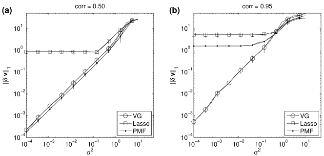
In this subsection we show the accuracy VG, Lasso and PMF as a function of the noise $\hat{\sigma}^{2}$. We generate data with $n=100,p=100,p_{v}=20$ and $\hat{w}_{i}=1$ for $20$ randomly chosen components $i$. We vary $\hat{\sigma}^{2}$ in the range $10^{-4}$ to $10$ for for two values of the correlation strength in the inputs $\zeta=0.5,0.95$.

For weakly correlated inputs, Fig. 5a., we distinguish three noise domains: for large noise all methods produce errors of ${\cal O}(1)$ and fail to find the predictive features. For intermediate and low noise levels, VG and PMF are significantly better than Lasso. In the limit of zero noise, the error of VG and PMF keeps on decreasing whereas the Lasso error saturates to a constant value.

For strongly correlated inputs, Fig. 5b., we observe that whereas the error of VG scales approximately as before, PMF gets stuck in local minima in some instances, yielding worse average performance than VG. See section 5 for a further discussion of this point.

Figure 5: Accuracy of VG, Lasso and PMF as a function of the noise. Errorbars of $\parallel\delta\vec{v}\parallel_{1}$ for $10$ different random instances. Data is generated using $n=100,p=100,p_{v}=20$ and $\hat{w}_{i}=1$ for $20$ randomly chosen components $i$. We consider two values of the correlation strength in the inputs: (a) weakly correlated inputs $\zeta=0.5$ and (b) strongly correlated inputs $\zeta=0.95$. For PMF we choose the best solution (the one with highest value of the bound) for $10$ different random initializations for each of the $10$ instances.

4.4 Analysis of consistency: VG vs Lasso

It is well-known that the Lasso method may yield inconsistent results when input variables are correlated. In Zhao:2006:MSC:1248547.1248637 , necessary and sufficient conditions for consistency are derived. In addition, they give a number of examples where Lasso gives inconsistent results. Their simplest example has three input variables, $x_{1},x_{2},x_{3}$. $x_{1},x_{2},\xi,e$ are independent and Normal distributed random variables, $x_{3}=2/3x_{1}+2/3x_{2}+\xi$ and $y=\sum_{i=1}^{3}\hat{w}_{i}x_{i}+e$, $p=1000$. When $\hat{w}=(-2,3,0)$ (Example b) this example is consistent, but when $\hat{w}=(2,3,0)$ (Example a) this example violates the consistency condition. The Lasso and VG solution for Example a for different values of $\lambda$ and $\gamma$ are shown in fig. 6a,b, respectively. The VG solution $v_{i}=m_{i}w_{i}$ in terms of $m_{i}$ and $w_{i}$ is shown in fig. 6c,d.

Figure 6: (Color online) Lasso and VG solution for the inconsistent Example a of Zhao:2006:MSC:1248547.1248637 . Top left: Lasso solution versus $\lambda$ is called inconsistent because it does not contain a $\lambda$ for which the correct sparsity ($w_{1,2}\neq 0,w_{3}=0$) is obtained. Top right: the VG solution for $\vec{v}$ versus $\gamma$ contains large range of $\gamma$ for which the correct solution is obtained. Bottom left: VG solution for $\vec{m}$ (curves for $m_{1,2}$ are identical). Bottom right: VG solution for $\vec{w}$.

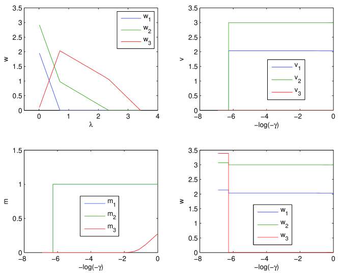
The average results over 100 instances for Example a and Example b are shown in table 3.

	Example a		Example b
	$\|\delta\vec{v}\|_{1}$	$\max(|v_{3}|)$	$\|\delta\vec{v}\|_{1}$	$\max(|v_{3}|)$
Ridge	$0.64\pm 0.18$	$0.48$	$0.02\pm 0.02$	$0.27$
Lasso	$0.19\pm 0.14$	$0.30$	$0.00\pm 0.00$	$0.00$
VG	$0.05\pm 0.03$	$0.00$	$0.00\pm 0.00$	$0.00$

Table 3: Accuracy of Ridge, Lasso and VG for Example 1a,b from Zhao:2006:MSC:1248547.1248637 . $p=p_{v}=1000$. Parameters $\lambda$ (Ridge and Lasso) and $\gamma$ (VG) optimized through cross validation. $\|\delta\vec{v}\|_{1}$ as before, $\max(|v_{3}|)$ is maximum over $100$ trials of the absolute value of $v_{3}$. Example a is inconsistent for Lasso and yields much larger errors than the VG. Example b is consistent and the quality of the Lasso and VG are similar. Ridge regression is bad for both examples.

We see that the VG does not suffer from inconsistency and always finds the correct solution. This is remarkable as one might have feared that the non-convexity of the VG would result in sub-optimal local minima.

4.5 Boston-housing dataset: VG vs PMF

We now focus on comparing in more detail the performance of VG with PMF. In titsias2012 , the Boston-housing dataset is used to test the accuracy of the PMF approximation.

This is a linear regression problem that consists of $456$ training examples with one-dimensional response variable $y$ and $13$ predictors that include housing values. We use here the same setup as in titsias2012 to compare VG with PMF. For PMF, hyperparameters were fixed to values $\sigma=0.1\times\text{var}(y),\pi=0.25,\sigma_{w}=1$ where var(y) denotes the output variance. For the VG, we use $\beta=1/\sigma^{2}$, $\gamma=\log(\pi/(1-\pi))$ and hyperparameter $\sigma_{w}$ is implicitly equal to $\infty$ in the VG (see Appendix C for details of how both models compare). Since $\gamma$ and $\beta$ are given, the VG algorithm reduces to iterate eqs. (8) and (9) starting from a random $\vec{m}$. Similarly, the PMF reduces to perform an E-step given the fixed hyperparameter values.

As in titsias2012 , we use random initial values for the variational parameters between $0$ and $1$ (soft initialization) and random values equal to $0$ or $1$ (hard initialization). We considered as ground truth $\hat{w}\equiv\vec{w}^{\text{tr}}$ the result of the efficient paired Gibbs sampler developed in titsias2012 .

	soft-error	extreme-error
PMF titsias2012	0.208 [0.002, 0.454]	0.204 [0.002, 0.454]
PMF	0.237 [0.001, 0.454]	0.209 [0.001, 0.454]
VG	0.006 [0.006, 0.006]	0.006 [0.006, 0.006]

Table 4: Comparison of VG and PMF in the Boston-housing dataset in terms of approximating the ground-truth $\hat{w}$. Average errors $\|\delta\vec{v}\|_{1}=\sum_{i=1}^{n}|v_{i}-\hat{w}_{i}|$ , with $v_{i}$ the approximation of VG or PMF, together with $95\%$ confidence intervals (given by percentiles) obtained after $300$ random initializations for both soft and extreme initializations.

Table 4 shows the results. The first and second rows show the errors reported in titsias2012 and the errors that we obtain using their software, respectively. We observe a small discrepancy in the average errors. However, if we consider the percentiles, the results are consistent. In practice, what we observe is that PMF finds two local optima depending on the initialization: one is the correct solution (error $\approx 10^{-3}$) whereas the other has error $0.454$. These two solutions are found equally often for both soft or hard initializations, showing no dependence on the type of initialization, in agreement with titsias2012 .

The results of VG are shown on the third row. Contrary to PMF, the VG shows no dependence on the initialization and always finds a solution with an error of order $10^{-3}$. These results give evidence that the combined variational/MAP approach of VG can be better than PMF avoiding local minima.

4.6 Dependence on the Number of Samples

We now analyze the performance of all considered methods as a function of the proportion of samples available. We first analyze the case when inputs are not correlated and then consider correlations of practical relevance that appear in genetic datasets.

For these experiments, we generate the data for dimension $n=500$ and noise level $\beta=1$. We explore two scenarios: very sparse problems with only $10\%$ of active predictors and denser problems with $25\%$ of active predictors. The weights of the active predictors are set to $1$.

4.6.1 Uncorrelated Case

Figure 7: Uncorrelated case: Performance as a function of number of training samples $p$ for two levels of sparsity ($10\%$ and $25\%$ of non-zero entries). For each value averages over $20$ runs are plotted. Top: area under the ROC curves (see text for definition). Middle: reconstruction error, defined as $\|\delta\vec{v}\|_{1}=\sum_{i=1}^{n}|v_{i}-\hat{w}_{i}|$. Bottom: generalization error, defined as the MSE in the test set. For all methods except for PMF, train set size is $p$ and validation sets size $p_{v}=p/30$. For PMF the training set has size $p+p_{v}$. Lowest curve shows theoretically optimal generalization error obtained by using the target weights from which the data is generated.

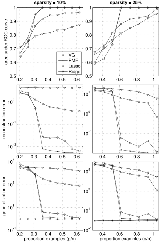
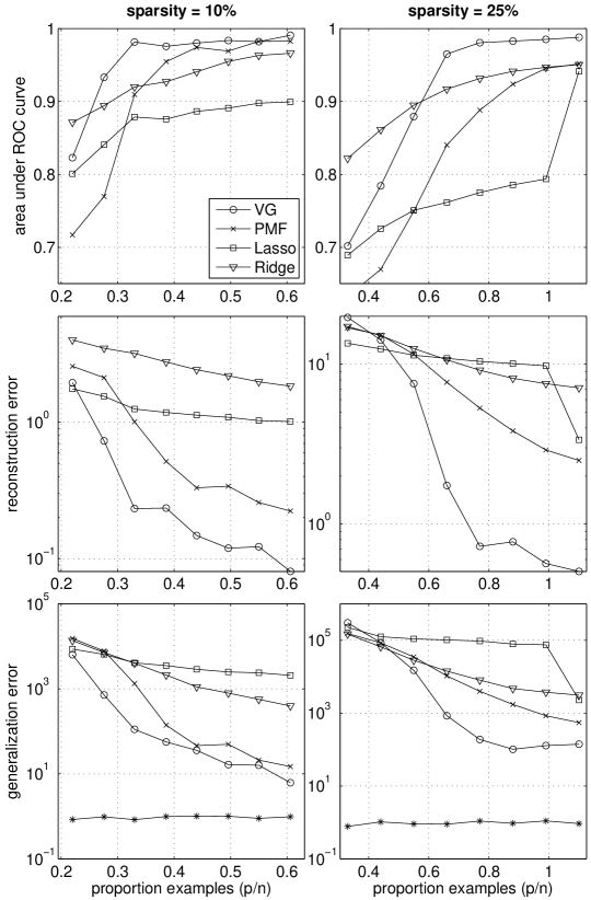
Figure 7 shows results of performance for uncorrelated inputs. Top plots show the area under the Receiver Operating Characteristic (ROC) curve. The ROC curve is calculated by thresholding the weight estimates. Those weights that lie above (below) the threshold are considered as active (inactive) predictors. The ROC curve plots the fraction of true positives versus the fraction of false positives for all threshold values. The area under the curve measures the ability of the method to correctly classify those predictors that are and are not active. A value of 1 for the area represents a perfect classification whereas 0.5 represents random classification. The ROC is plotted as a function of the fraction of samples relative to the number of inputs: $p/n$.

For both VG and PMF, we observe in all performance measures a transition from a regime where solutions are poor to a regime with almost perfect recovery. This transition, not noticeable in the other (convex) methods, occurs at around $35\%$ of examples for $10\%$ of sparsity (left column) and shifts to higher values for denser problems ($\approx 60\%$ for $25\%$ of sparsity, right column).

If we compare VG with PMF we see that in the regime where both methods perform well, PMF performs slightly better than VG in terms of reconstruction error but their performance is identical in terms of the area under the ROC curve. The difference between VG and PMF is slightly more pronounced for denser problems. We also see that Lasso performs better than Ridge regression, but the difference between both methods tends to be smaller for denser problems. Both Lasso and ridge regression are significantly worse than VG and PMF.

4.6.2 Correlated case: Genetic dataset

Figure 8: Correlated case: (LEFT) (Color online) Example of input correlation matrix. (RIGHT) Performance as a function of number of training samples $p$ for two levels of sparsity ($10\%$ and $25\%$ of non-zero entries). For each value averages over $20$ runs are plotted. Top: area under the ROC curves (see text for definition). Middle: reconstruction error, defined as $\|\delta\vec{v}\|_{1}=\sum_{i=1}^{n}|v_{i}-\hat{w}_{i}|$. Bottom: generalization error, defined as the MSE in the validation set. For all methods except for PMF, train set size is $p$ and validation sets size $p_{v}=p/10$. For PMF the training set has size $p+p_{v}$.

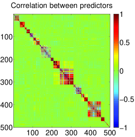
We now consider correlated inputs. We use input data obtained from a genetic domain, where inputs $x_{i}$ denote single nucleotide polymorphisms (SNPs) that have values $x_{i}=\{0,1,2\}$. SNPs typically show correlations structured in blocks, where nearby SNPs are highly correlated, but show no dependence on distant SNPs. An example of such correlation matrix can be seen in Figure 8 (left). The output data are generated as above.

Figure 8 (right) shows the results. Contrary to the uncorrelated case, the existence of strong correlations between some of the predictors prevents a clear distinction between solution regimes as a function of training set size. We observe, as before, that both VG and PMF are the preferable methods for sufficiently large training set size. In the three performance measures considered, VG performs better or comparable to PMF. Interestingly, the difference between VG and PMF becomes more significant for denser problems, when we expect more difficulty due to more presence of local minima.

4.7 Scaling with dimension $n$

Figure 9: Scaling with $n$: performance of VG, PMF and Lasso as a function of the number of features $n$. Data are generated as in Example 2. $p=100,p_{v}=100,\beta=2,\zeta=0$.

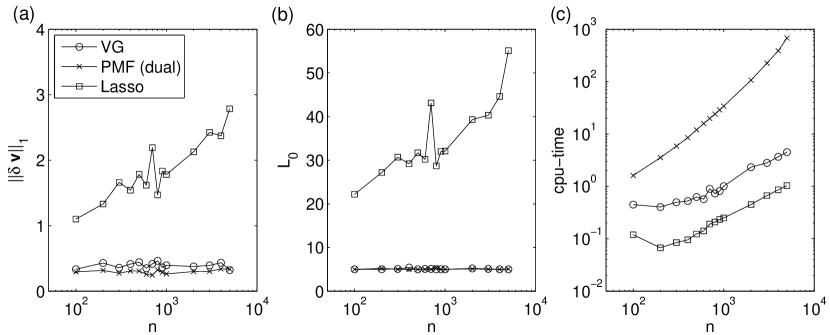
We conclude our empirical study by analyzing how the methods scale, both in terms of the quality of the solution as in terms of CPU times, as a function of the number of features $n$ for a constant number of samples. We use the data as in Example 2 above, with uncorrelated inputs.

Figure 9 shows the results for VG, PMF and Lasso. For the VG, we use the dual method described in the appendix B. Fig. 9a shows that the VG and PMF have constant quality in terms of the error $\|\delta\vec{v}\|_{1}$, whereas the quality of the Lasso deteriorates with $n$. Fig. 9b shows that the VG and PMF have close to optimal norms $L_{0}=5$ and that the $L_{0}$ norm of the Lasso deteriorates with $n$. Fig. 9c shows that the computation time of all methods scales approximately linear with $n$. Lasso is significantly faster than VG and PMF, and VG is significantly faster than PMF. Note, however that the VG and the PMF methods are implemented in Matlab whereas the Lasso method uses an optimized Fortran implementation.

5 Discussion

In this paper, we have introduced a new variational method for sparse regression using $L_{0}$ penalty. We have presented a minimal version of the model with no (hierarchical) prior distributions to highlight some important features: the variational ridge term that dynamically regularizes the regression; the input-output behavior as a smoothed version of hard feature selection; a phase plot that shows when the variational solution is unique in the orthogonal design case for different $p,\rho,\gamma$. We have also shown numerically that the VG is efficient and accurate and yields results that significantly outperform other considered methods.

The VG suffers from local minima as can be expected for any method that needs to solve a non-convex problem, like the PMF. From the numerical experiments we can conclude that VG is on average preferable to PMF in practical scenarios with strongly correlated inputs and/or moderately sparse problems, where the local minima problem is more severe. Although we have no principled solution for the local minima problem, we think that the combined variational/MAP approach together with the the annealing procedure that results from increasing $\gamma$, followed by a ”heating” phase to detect hysteresis works well in practice, helping to avoid local minima. Another obvious approach is to use multiple restarts or using more powerful approximations, such as structured mean field approximation or belief propagation. We remark that the PMF in the general setting titsias2012 includes an extra layer of flexibility that can be used to capture correlations between input variables. Such extensions can also be considered for VG.

We have not explored the use of different priors on $\vec{w}$ or on $\beta$. In addition, a prior could be imposed on $\gamma$. It is likely that for particular problems the use of a suitable prior could further improve the results.

We have seen that the performance of the VG is excellent in the zero noise limit. In this limit, the regression problem reduces to a compressed sensing problem candes2005 ; donoho2006 . The performance of compressed sensing with $L_{q}$ sparseness penalty was analyzed theoretically in kabashima2009 , showing the superiority of the $L_{1}$ penalty in comparison to the $L_{2}$ penalty and suggesting the optimality of the $L_{0}$ penalty. Our numerical result are in agreement with this finding.

Our implementation uses parallel updating of Eqs. 8-10, or Eqs. 8,21, 24-27 when using the dual formulation. One may consider also a sequential updating. This was done successfully for the Lasso based on the idea of the Gauss-Seidel algorithm friedman2009 . The advantage of such an approach is that each update is linear in both $n$ and $p$, since only the non-zero components need to be updated. However, the number of updates to converge will be larger. The proof of convergence for such a coordinate descend method for the VG is likely to be more complex than for the Lasso due to non-convexity. As a result, a smoothing parameter $\eta\neq 1$ (see Algorithm 1) may still be required.

Acknowledgments

We would like to thank M. Titsias for providing the code of PMF and specially the Boston Housing files. We also thank Kevin Sharp and Wim Wiegenrick for useful discussions and anonymous reviewers for helping on improving the manuscript.

Appendix A : Phase plot computation for the orthogonal case

In the uni-variate case, $f(m)$ in Eq. 14 is an increasing function of $m$ and crosses the line $m$ either 1 or three times, depending on the values of $p$ and $\gamma$ (see fig. 10). In the multivariate orthogonal case, this is still true, since the influence of other features is only through $\beta$. We can thus write $\beta^{-1}=\sigma_{y}^{2}(1-\rho m-\delta)$, where $0\leq\delta<1$ is a function of the variational parameters of the other features.

Figure 10: (Color online) $f(m)$ vs $m$. Left (a): $p=100,\gamma=-10$, different lines correspond to different values of $0<\rho<1$ (higher lines are higher $\rho$). The solution for $m$ is given by the intersection $f$ with the diagonal line. The solution for $m$ is unique and increases with increasing $\rho$. Right (b): Same as left, but with $p=100,\gamma=-30$. Depending on $\rho$, there are one or three solutions for $m$. The solutions close to $m\approx 0,1$ correspond to local minima of $F$. The intermediate solution corresponds to a local maximum of $F$.

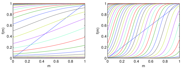
Thus, there are regions of parameter space $\gamma,p,\rho$ where the uni-variate solution is unique and others for which there are two stable solutions.

The transition between these two regions is when $f^{\prime}(m)=1$ and $f(m)=m$. These two equations imply

$$\left(1+\frac{p}{2}\right)\rho^{2}m^{2}-\left(2\rho(1-\delta)+\frac{p}{2}\rho^{2}\right)m+(1-\delta)^{2}=0$$ (16)

This quadratic equation in $m$ has either zero, one or two solutions, corresponding to no touching, touching once and touching twice, respectively. Denote $a=(1+\frac{p}{2})\rho^{2},b=2\rho(1-\delta)+\frac{p}{2}\rho^{2}$. The critical value for $\rho,p$ is when Eq. 16 has one solution for $m$, which occurs when

$$D = b^{2}-4a(1-\delta)^{2}=\frac{p}{2}\rho^{2}\left(\rho-\rho^{*}\right)\left(\frac{p}{2}\rho+2(1-\delta)+2(1-\delta)\sqrt{1+\frac{p}{2}}\right)=0$$

$$\rho^{*} = \frac{4}{p}(1-\delta)\left(\sqrt{1+\frac{p}{2}}-1\right)$$ (17)

Thus, $D$ is positive when $\rho>\rho^{*}$ and Eq. 16 has two solutions for $m$. We denote these solutions by $m_{1,2}=\frac{b\pm\sqrt{D}}{2a}$. Note, that the solutions in these critical points only depend on $\rho,p$. For each of these solutions we must find a $\gamma$ such that $f(m)=m$, which is given by

$$\gamma_{i} = \log\frac{m_{i}}{1-m_{i}}-\frac{p}{2}\frac{\rho}{1-\rho m_{i}}\qquad i=1,2$$ (18)

It is easy to see that the smallest of these solutions $m_{1}<m_{2}$ corresponds to a local maximum of the free energy and can be discarded. Thus, when $\rho>\rho^{*}$ and $\gamma_{2}<\gamma<\gamma_{1}$ two stable variational solutions $m\approx 0,1$ co-exist.

When $\rho<\rho^{*}$, Eq. 16 has no solutions for $m$. In this case the conditions $f^{\prime}(m)=1$ and $f(m)=m$ cannot be jointly satisfied and the variational solution is unique.

From Eq. 17 we see that $\rho^{*}$ is a decreasing function of $p$ and when $p\gg 1$, $\rho^{*}\approx 2\sqrt{\frac{2}{p}}$. In the critical point, where $\rho=\rho^{*}(p)$, $m=b/2a\approx\frac{1}{2}\left(1+\sqrt{\frac{2}{p}}\right)$ and

$$\gamma^{*}\approx-\sqrt{2p}(1-\delta)$$ (19)

When $\rho<\rho^{*}$ or $\gamma>\gamma^{*}$ the variational solution is unique. We illustrate the phase plot $\rho,\gamma$ for $p=100$ in fig. 1a.

Appendix B : Dual Formulation

The solution of the system of Eqs. 8-10 by fixed point iteration requires the repeated solution of the $n$ dimensional linear system $\chi^{\prime}\vec{w}=\vec{b}$. When $n>p$, we can obtain a more efficient method using a dual formulation.

We define new variables $z^{\mu}=\sum_{i}m_{i}w_{i}x_{i}^{\mu}$ and add Lagrange multipliers $\lambda^{\mu}$:

$$F = -\frac{p}{2}\log\frac{\beta}{2\pi}+\frac{\beta}{2}\sum_{\mu}^{p}(z^{\mu}-y^{\mu})^{2}+\frac{\beta p}{2}\sum_{i}m_{i}(1-m_{i})w_{i}^{2}\chi_{ii}$$ (20)

$$- \gamma\sum_{i=1}^{n}m_{i}+\sum_{i=1}^{n}\left(m_{i}\log m_{i}+(1-m_{i})\log(1-m_{i})\right)$$

$$+ \sum_{\mu}\lambda^{\mu}(z^{\mu}-\sum_{i}m_{i}w_{i}x_{i}^{\mu})$$

We compute the derivatives of Eq. 20:

$$\frac{\partial F}{\partial w_{i}} = m_{i}\left(\beta p(1-m_{i})\chi_{ii}w_{i}-\sum_{\mu}\lambda^{\mu}x_{i}^{\mu}\right)$$

$$\frac{\partial F}{\partial z^{\mu}} = \beta(z^{\mu}-y^{\mu})+\lambda^{\mu}$$

$$\frac{\partial F}{\partial\beta} = -\frac{p}{2\beta}+\frac{1}{2}\sum_{\mu}^{p}(z^{\mu}-y^{\mu})^{2}+\frac{p}{2}\sum_{i}m_{i}(1-m_{i})w_{i}^{2}\chi_{ii}$$

$$\frac{\partial F}{\partial m_{i}} = \frac{\beta p}{2}(1-2m_{i})w_{i}^{2}\chi_{ii}-\gamma+\sigma^{-1}(m_{i})-\sum_{\mu}\lambda_{\mu}w_{i}x_{i}^{\mu}$$

$$\frac{\partial F}{\partial\lambda^{\mu}} = z^{\mu}-\sum_{i}m_{i}w_{i}x_{i}^{\mu}$$

By setting $\frac{\partial F}{\partial w_{i}}=\frac{\partial F}{\partial z^{\mu}}=0$ we obtain

$$w_{i} = \frac{1}{\beta p\chi_{ii}}\frac{1}{1-m_{i}}\sum_{\mu}\lambda^{\mu}x_{i}^{\mu}$$ (21)

and $z^{\mu}=y^{\mu}-\frac{1}{\beta}\lambda^{\mu}$. Setting the remaining derivatives to zero, and eliminating $w_{i}$ and $z^{\mu}$ we obtain Eq. 8 and

$$\beta = \frac{1}{p}\sum_{\mu\nu}\lambda_{\mu}\lambda_{\nu}A_{\mu\nu}$$ (22)

$$\beta y^{\mu} = \sum_{\nu}A_{\mu\nu}\lambda^{\nu}$$ (23)

with $A_{\mu\nu}$ given by

$$A_{\mu\nu} = \delta_{\mu\nu}+\frac{1}{p}\sum_{i}\frac{m_{i}}{1-m_{i}}\frac{x_{i}^{\mu}x_{i}^{\nu}}{\chi_{ii}}$$ (24)

For given $A_{\mu\nu}$, let $\hat{y}$ denote the solution of

$$\sum_{\nu=1}^{p}A_{\mu\nu}\hat{y}^{\nu} = y^{\mu}$$ (25)

Then it is easy to verify that

$$\frac{1}{\beta} = \frac{1}{p}\sum_{\mu}\hat{y}^{\mu}y^{\mu}$$ (26)

$$\lambda^{\mu} = \beta\hat{y}^{\mu}$$ (27)

solve the system of Eqs. 22-23.

Appendix C : Relation with the Paired-Mean Field approximation

The VG shares many similarities with the recently proposed paired mean field (PMF) variational approach [1]. Here we relate both approaches in terms of three different aspects: the probabilistic model, the variational approximation and the optimization algorithm.

Model

: The model considered for the PMF variational approximation is defined for multiple outputs and considers a linear combination of basis functions governed by a Gaussian process. To relate this model to the one presented in this work, we consider the one-dimensional output without the extra input layer.

The spike and slab model [5] considers a linear regression model of the form:

$$y =\sum_{i=0}^{n}\hat{v}_{i}x_{i}+\xi$$

$$\hat{v}_{i} \sim\pi\mathcal{N}(\hat{v}_{i}|0,\sigma^{2}_{w})+(1-\pi)\delta_{0}(\hat{v}_{i}),\qquad\forall i.$$

That is, the prior over the weights is factorized, with each weight distributed according to a mixture distribution: with probability $\pi$, each $\hat{v}_{i}$ is drawn from a Gaussian centered at zero with variance $\sigma^{2}_{w}$, and with probability $1-\pi$, each $\hat{v}_{i}$ is zero. The sparsity of the solution is controlled by $\pi$, either directly or by specifying a prior over $\pi$.

Observe that we can equivalently write $\hat{v}_{i}$ as the product of a Bernoulli random variable $s_{i}\sim\pi^{s_{i}}(1-\pi)^{1-s_{i}}$ and a Gaussian random variable $w_{i}\sim\mathcal{N}(w_{i}|0,\sigma_{w}^{2})$, which is the reparameterization used in [1].

To relate the model used in the VG defined by Eqs. (2) and (4) to the previous one we make the following identifications:

• The prior on $w_{i}$ is flat, which corresponds to setting $\sigma_{w}=\infty$ in [1].

• $\gamma=\log(\pi/(1-\pi))$.

Thus, the spike and slab model [5] and the model considered by [1] are identical and both models are identical to the model considered in this paper when a Gaussian prior is placed over the weights.

Variational approximation

: The PMF variational distribution places each weight $w_{i}$ and bit $s_{i}$ in the same factor:

$$q(\vec{w},\vec{s}) =\prod_{i=1}^{n}q_{i}(w_{i},s_{i}).$$ (28)

On the contrary, the VG reduces to the classical factorized variational approach under the restriction that the posterior for the weight is a delta function.

Algorithm

: The optimization in [1] uses an EM algorithm that alternates between expected values of the latent variables $\vec{w},\vec{s}$ (E-Step) and optimization of hyperparameters $\{\sigma_{y}^{2},\sigma^{2}_{w},\pi\}$ (M-Step).

The VG method differs mainly in two points. The VG method:

• Computes expectation of $\vec{s}$ (denoted by $\vec{m}$) but finds MAP solution for $\vec{w}$.

• Searches the space of solutions using a forward and a backward sequential search over hyperparameter $\gamma$ using a validation set. For a given $\gamma$, the rest of the parameters are optimized using a training set and initialized with a ’warm’ solution from the previous step (see Algorithm 1).

References

- (1) M. Titsias and M. Lázaro-Gredilla. Spike and Slab Variational Inference for Multi-Task and Multiple Kernel Learning. In Advances in Neural Information Processing Systems 24, pages 2339–2347, 2011.
- (2) R. Tibshirani. Regression shrinkage and selection via the Lasso. Journal of the Royal Statistical Society B, 58(1):267–288, 1996.
- (3) J. H. Friedman, T. Hastie, and R. Tibshirani. Regularization paths for generalized linear models via coordinate descent. Journal of Statistical Software, 33(1):1–22, 2 2010.
- (4) I. E. Frank and J. H. Friedman. A statistical view of some chemometrics regression tools. Technometrics, 35(2):109–135, 1993.
- (5) E. I. George and R. E. McCulloch. Variable Selection Via Gibbs Sampling. Journal of the American Statistical Association, 88(423):881–889, 1993.
- (6) B. A. Logsdon, G. E. Hoffman, and J. G. Mezey. A variational Bayes algorithm for fast and accurate multiple locus genome-wide association analysis. BMC Bioinformatics, 11:58, 2010.
- (7) R. Yoshida and M. West. Bayesian learning in sparse graphical factor models via variational mean-field annealing. Journal of Machine Learning Research, 99(Aug):1771–1798, 2010.
- (8) D. Hernández-Lobato, J. M. Hernández-Lobato, T. Helleputte, and P. Dupont. Expectation propagation for bayesian multi-task feature selection. In Proceedings of the 2010 European conference on Machine learning and knowledge discovery in databases: Part I, pages 522–537. Springer-Verlag, 2010.
- (9) M. I. Jordan, Z. Ghahramani, T. S. Jaakkola, and L. K. Saul. An introduction to variational methods for graphical models. Machine Learning, 37(2):183–233, 1999.
- (10) H. J. Kappen and J. J. Spanjers. Mean field theory for asymmetric neural networks. Physical Review E, 61:5658–5663, 2000.
- (11) K. P. Murphy, Y. Weiss, and M. I. Jordan. Loopy Belief Propagation for approximate inference: An empirical study. In Proceedings of the 15th Annual Conference on Uncertainty in Artificial Intelligence, pages 467–475. Morgan Kaufmann Publishers, 1999.
- (12) M. Opper and D. Saad. Advanced Mean Field Methods: Theory and Practice. MIT press, 2001.
- (13) M. J. Wainwright and M. I. Jordan. Graphical models, exponential families, and variational inference. Foundations and Trends in Machine Learning, 1(1-2):1–305, 2008.
- (14) D. Barber and W. Wiegerinck. Tractable variational structures for approximating graphical models. In Advances in Neural Information Processing Systems II, pages 183–189. MIT Press, 1999.
- (15) L. Breiman. Better subset regression using the nonnegative garrote. Technometrics, 37(4):373–384, 1995.
- (16) T. J. Mitchell and J. J. Beauchamp. Bayesian variable selection in linear regression. Journal of the American Statistical Association, 83(404):pp. 1023–1032, 1988.
- (17) P. Zhao and B. Yu. On Model Selection Consistency of Lasso. Journal of Machine Learning Research, 7(Dec):2541–2563, 2006.
- (18) E. J. Candes and T. Tao. Decoding by linear programming. IEEE Transactions on Information Theory, 51(12):4203–4215, December 2005.
- (19) D. L. Donoho. Compressed sensing. IEEE Transactions on Information Theory, 52(4):1289–1306, 2006.
- (20) Y. Kabashima, T. Wadayama, and T. Tanaka. A typical reconstruction limit for compressed sensing based on -norm minimization. Journal of Statistical Mechanics: Theory and Experiment, 2009(09):L09003, 2009.