Maximizing the statistical diversity of an ensemble of bred vectors
by using the geometric norm

Abstract

We show that the choice of the norm has a great impact on the construction of ensembles of bred vectors. The geometric norm maximizes (in comparison with other norms like the Euclidean one) the statistical diversity of the ensemble while, at the same time, enhances the growth rate of the bred vector and its projection on the linearly most unstable direction, i.e. the Lyapunov vector. The geometric norm is also optimal in providing the least fluctuating ensemble dimension among all the spectrum of $q$-norms studied. We exemplify our results with numerical integrations of a toy model of the atmosphere (the Lorenz-96 model), but our findings are expected to be generic for spatially extended chaotic systems.

[J.Atmos.Sci.68,1507–1512(2011)]©Copyright July 2011 AMS

I Introduction

The ‘breeding method’ is a well-established and computationally inexpensive procedure for generating perturbations for ensemble integrations (Toth and Kalnay, 1993, 1997). Bred vectors (BVs) are finite perturbations periodically rescaled to a certain magnitude that have been prominently used in probabilistic weather forecasting with ensembles (Kalnay, 2002; Gneiting and Raftery, 2005). The breeding method and variants of it are applied in operative ensemble forecast systems, such as National Centers for Environmental Predictions (NCEP, USA), see e.g. Wei et al. (2008). Moreover, breeding continues to be a popular tool to study the predictability of a variety of systems such as the baroclinic rotating annulus (Young and Read, 2008) or the atmosphere of Mars (Newman et al., 2004).

Different initial BV perturbations all generally tend to become aligned with the fastest growing modes. If different BVs were globally quasi-orthogonal to each other (Toth and Kalnay, 1997), one might expect they would automatically provide a good sample of the different dominant growing error directions, without the need for additional computation. A closer inspection reveals that the BV perturbations are often locally rather similar in shape, differing only in sign and amplitude (Toth and Kalnay, 1997; Hallerberg et al., 2010). In fact, a major modification of the BV implementation at NCEP has recently been implemented by replacing the BVs given by the ensemble forecast with some ‘ensemble transform’ that orthogonalizes the ensemble with respect to the metric defined by the inverse covariance matrix (Bishop and Toth, 1999; Wang and Bishop, 2003; Wei et al., 2006, 2008). Other metrics can be used and lead to different ensembles of BVs (Keller et al., 2010). Orthogonalization with respect to a given metric generally enhances the statistical diversity of the ensemble by making the BV perturbations globally more dissimilar (Annan, 2004; Keller et al., 2010).

In this paper we show how the ensemble diversity can be enhanced by using the geometric norm with no further transforms or orthogonalizations needed. We first show that the BVs dynamics and the statistical properties of the ensemble strongly depend on the norm definition used to construct them. So far Euclidean-type norms are widely used in applications. However, our results demonstrate that, among a spectrum of studied norms, the geometric norm is the most convenient because it provides a greater statistical diversity of the ensemble, while it enhances the projection of the ensemble as a whole on the most unstable direction. With other norm choices, like the standard Euclidean one, a good projection on the leading Lyapunov vector (LV) is always associated with the collapse of all the BVs, i.e. the complete loss of the ensemble diversity.

II The model

We illustrate our study with numerical integrations of the well-known Lorenz-96 model (Lorenz, 1996) that has been used by various authors as a low order testbed for atmospheric prediction and assimilation studies (Lorenz and Emanuel, 1998; Anderson, 2001). This model is defined by the set of variables $\{u(x,t)\}_{x=1,\ldots,L}$ and evolves according to

$$\frac{d\,u(x,t)}{dt} = -u(x-1,t)\left[u(x-2,t)-u(x+1,t)\right]$$ (1)

$$- u(x,t)+F,\quad\mbox{with}\quad x=1,...,L.$$

with periodic boundary conditions in the discrete spatial variable $x$. Hereafter we adopt a system size of $L=128$ and a forcing constant $F=8$. For these values the system exhibits well developed chaos (Lorenz, 2006).

A good description of the chaotic dynamics can be achieved by understanding the behavior of initial infinitesimal perturbations, which are governed by the ‘tangent linear model’:

$$\frac{d\,\delta u(x,t)}{dt}=-\delta u(x-1,t)\left[u(x-2,t)-u(x+1,t)\right]$$

$$-u(x-1,t)\left[\delta u(x-2,t)-\delta u(x+1,t)\right]-\delta u(x,t).$$ (2)

After some transient any infinitesimal perturbation $\delta u(x,0)$ becomes permanently aligned along the most unstable direction. This direction defines, disregarding an arbitrary nonzero constant factor, the leading LV, and hereafter denoted $\mathbf{g}(t)=\{g(x,t)\}_{x=1,\ldots,L}$.

Obtaining the tangent linear (and adjoint) models can be however extremely difficult in operative weather models and one has to resort to analyzing finite perturbations, which are evolved with the full nonlinear model. This is for instance the situation at NCEP, where ensembles of BVs are used.

III Bred vectors

BVs are finite perturbations obtained after periodic rescaling, say at times $t_{m}=mT$ ($m\in\mathbb{Z}^{+}$). A control trajectory $\mathbf{u}$ and a perturbed one $\mathbf{u}^{\prime}$, are simultaneously integrated [via Eq. (1)] and at the scheduled times the difference between them is calculated

$$\mathbf{\Delta u}(t_{m})=\mathbf{u}^{\prime}(t_{m})-\mathbf{u}(t_{m})$$ (3)

and rescaled to a given amplitude $\varepsilon$, obtaining the BV

$$\mathbf{b}(t_{m})=\varepsilon\frac{\mathbf{\Delta u}(t_{m})}{\|\mathbf{\Delta u}(t_{m})\|}$$ (4)

This BV is then used to redefine the perturbed system:

$$\mathbf{u}^{\prime}(t_{m}^{+})=\mathbf{u}(t_{m})+\mathbf{b}(t_{m}).$$ (5)

with $t_{m}^{+}=\lim_{\nu\to 0}t_{m}+\nu$. The perturbed $\mathbf{u}^{\prime}$ and control $\mathbf{u}$ states are then evolved in time according to the model equations, Eq. (1), until the next scheduled rescaling. At the next scheduled time $t_{m+1}$ the breeding cycle, Eqs. (3)-(5), is repeated. After several breeding cycles, the perturbations generated by this procedure acquire a large growth rate, which makes them suitable for ensemble forecasting. Usually a set of BVs is evolved from different initial random perturbations and this constitutes the ensemble. Ideally a good ensemble of BVs should span the most unstable directions in phase space well enough to capture the main instabilities.

There are three basic ingredients in the definition of the BV: (i) the rescaling interval $T$, (ii) the perturbation amplitude $\varepsilon$, and (iii) the choice of the norm $\|\cdot\|$ used in Eq. (4).

The rescaling interval $T$ has a negligible influence in the results as long as it remains small —say, smaller than the doubling time, which is on the order of $0.4$ time units (t.u.) for the Lorenz-96 model. We have used $T=0.1$ t.u., which corresponds to $1/2$ day in the time scale assumed by Lorenz (1996).

The perturbation amplitude $\varepsilon$ controls the “finiteness” of the perturbations; a sufficiently small $\varepsilon$ makes the perturbation quasi-infinitesimal, and in the limit $\varepsilon\to 0$ the BV perfectly aligns with the leading LV of the system.

However, very little is known about the effect of the norm choice on the properties of the resulting ensemble and we discuss this issue in detail in the incoming sections.

IV Choice of a norm

The choice of the norm is probably the more obscure element determining the BVs’ nature. BVs have often been claimed to be insensitive to the choice of norm (Kalnay et al., 2002; Corazza et al., 2003). However, this belief is not actually based on any rigorous argument. Here we show that the effect of changing the norm type has a dramatic impact on BVs. We will show that different norms lead to different ensemble properties and it is not a mere change of the ‘ruler’ or metrics. There are intrinsic and genuine effects on the statistics of the BVs for each particular norm type.

Intuitively, for a homogeneous system like the Lorenz-96 model, any definition for the norm one wants to use should be homogeneous in the sense that it weights equally all sites. To see why this constraint is relevant let us consider a particularly illustrative example. Think of a norm arising from some scalar product $\|\mathbf{b}\|^{2}=\left<\mathbf{b},\mathbf{b}\right>=\mathbf{b}^{\rm T}\bm{\mathsf{M}}\mathbf{b}$ with a very “unbalanced” metric matrix $\bm{\mathsf{M}}$, e.g. $\bm{\mathsf{M}}=\rm{diag}(100,1,1,\ldots,1)$. This choice would result in very dissimilar BVs depending if the site $x=1$ is more or less unstable at a given time. For a given $\varepsilon$, at some times the vector dynamics could be infinitesimal-like while at other moments it would be clearly finite. For spatially homogeneous systems, it is reasonable to restrict ourselves to “homogeneous“ norms that produce a BV that is statistically equivalent up to a high degree at different times and we do so in our study.

In this work we compare the performance of $q$-norms, which are defined as

$$\|\mathbf{\Delta u}\|_{q}=\left[\frac{1}{L}\sum_{x=1}^{L}|{\Delta u}(x,t)|^{q}\right]^{1/q}$$ (6)

Note that for $q=2$ the norm is an energy-like norm, analogous to those used in atmospheric models. In the limit $q\to\infty$ the $q$-norm becomes the supremum norm:

$$\|\mathbf{\Delta u}\|_{q\to\infty}=\sup\{|{\Delta u}(x,t)|\}_{x=1,\ldots,L}.$$ (7)

Moreover, the geometric mean is obtained in the limit $q\to 0$:

$$\|\mathbf{\Delta u}\|_{0}=\prod_{x=1}^{L}\left|\Delta u(x,t)\right|^{1/L}$$ (8)

The use of the geometric norm yields the so-called logarithmic BVs (Primo et al., 2005, 2006, 2008; Pazó et al., 2010; Hallerberg et al., 2010). For clarity of presentation we will add the subscript $q$ to the notation (for the BV, $\mathbf{b}_{q}$, and the amplitude, $\varepsilon_{q}$) to emphasize which $q$-norm is being used. For all $q$-norms the BVs look like very similar to the naked eye is strongly localized in space, and are strongly localized in space for small $\varepsilon_{q}$. (see for instance Hallerberg et al. (2010) and Primo et al. (2008) for typical snapshots of BVs with $q=0$ and $q=2$).

Along this paper we shall be considering an ensemble of $k=10$ BV members, $\{\mathbf{b}_{q}^{(i)}\}_{i=1,\ldots,k}$. All members of the ensemble are simultaneously rescaled, and they are initiated with independent random initial conditions, which is expected to result in some degree of diversity in the ensemble of BVs (Kalnay et al., 2002).

V Results

We define ensemble diversity as the degree of linear independence or transversality among the ensemble members. Diversity can be quantified by calculating the ‘ensemble dimension’, which measures the effective dimension of the sub-space spanned by the ensemble. The higher the ensemble dimension the greater the statistical diversity. Higher ensemble dimension would imply larger dissimilarities among the ensemble members. Since BV perturbations tend to align with the fastest growing modes, a greater diversity indicates that the ensemble is able to actually sample not only the main LV but also other, less unstable, directions.

Our goal here is to show, by means of several numerical calculations with a simple model, that the 0-norm is more convenient than other norms for constructing ensembles of BVs as far as ensemble diversity enhancement is concerned. We arrive to this conclusion measuring the ensemble dimension and its temporal fluctuations, the average growth rate, and the alignment of the ensemble members with the main LV.

V.1 Ensemble dimension

In this subsection we will analyze the statistical diversity in an ensemble of $k$ BVs. Clearly, for all $q$ values, in the limit $\varepsilon_{q}\to 0$ all BVs become aligned with the leading LV and there is no diversity in the ensemble (other than a global sign for the orientation of the vectors). If $\varepsilon_{q}$ is finite some degree of transversality between ensemble members can be expected, and to measure this diversity of the ensemble we resort to the so-called ensemble dimension (Bretherton et al., 1999).

Figure 1: Average ensemble dimension as a function of the amplitude $\varepsilon_{q}$ for ensembles of $k=10$ BVs, with different $q$-norms.

The ensemble dimension (Oczkowki et al., 2005) or BV dimension (Patil et al., 2001) was proposed as a way to account for the number of effective degrees of freedom that explains most of the total ensemble variance (in the spirit of principal component analysis), see e.g. Bretherton et al. (1999) and references therein. To compute the ensemble dimension at a given time one computes the $k\times k$ covariance matrix $\bm{\mathsf{C}}$ with elements:

$$C_{ij}(t)=\frac{\left<\mathbf{b}_{q}^{(i)},\mathbf{b}_{q}^{(j)}\right>}{L\|\mathbf{b}_{q}^{(i)}\|_{2}\|\mathbf{b}_{q}^{(j)}\|_{2}}.$$ (9)

where the standard scalar product is used in the numerator $\left<\mathbf{b}_{q}^{(i)},\mathbf{b}_{q}^{(j)}\right>=\sum_{x}b_{q}^{(i)}(x,t)b_{q}^{(j)}(x,t)$. If we denote by $\{\mu_{i}(t)\}_{i=1,\ldots,k}$ the set of eigenvalues of $\bm{\mathsf{C}}$, the ensemble dimension is:

$$D_{\mathrm{en}}(t)=\frac{\left(\sum_{i=1}^{k}\sqrt{\mu_{i}}\right)^{2}}{\sum_{i=1}^{k}\mu_{i}}$$ (10)

where the denominator ($\sum_{i}\mu_{i}$) equals $k$ due to the normalizing terms in the denominator of (9). The statistic (10) typically returns a real number between two limit values: $D_{\mathrm{en}}=k$ (if all vectors are orthogonal) and $D_{\mathrm{en}}=1$ (if all vectors are aligned). Therefore $D_{\mathrm{en}}(t)$ measures the instantaneous degree of “transversality” of the ensemble.

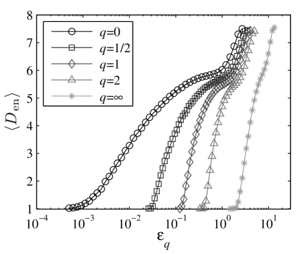
Figure 1 depicts the results of the time-average ensemble dimension $\left<D_{\mathrm{en}}\right>$ for different $q$-norms. Depending on the value of $q$ the amplitude $\varepsilon_{q}$ is varied in a different range. The largest value of $\varepsilon_{q}$ in each data set corresponds (approximately) to the value of the average distance (for the corresponding $q$-norm) between independent realizations of the model (i.e. random climatological values). In applications $\varepsilon_{q}$ is much smaller than this value (typically of the order of the analysis error). In the small $\varepsilon_{q}$ region of the plots, $\left<D_{\mathrm{en}}\right>$ becomes equal to 1 below a particular value of $\varepsilon_{q}$, though for the 0-norm the convergence to $1$ appears to be much less abrupt.

V.2 Fluctuations of the ensemble dimension

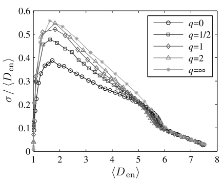
Figure 1 shows that all $q$-norms allow to obtain ensembles with a certain $\left<D_{\mathrm{en}}\right>$ after tuning $\varepsilon_{q}$ to a particular value. However the ensemble dimension is a time-fluctuating quantity and one should wish to minimize its fluctuations. Of course some degree of fluctuations is unavoidable due to (i) finiteness of the ensemble and (ii) intrinsic fluctuations in the state of the system (which progressively average out for large enough systems).

We characterize the fluctuations of $D_{\mathrm{en}}$ by means of the standard deviation $\sigma=\left<\left[D_{\mathrm{en}}(t)-\left<D_{\mathrm{en}}\right>\right]^{2}\right>^{1/2}$ where the brackets denote a temporal average. The results are depicted in Fig. 2, where we plot the relative fluctuations of the ensemble dimension versus $\left<D_{\mathrm{en}}\right>$ to better compare different $q$-norms. One can readily see that the 0-norm produces the ensemble with the smallest fluctuations for most $\left<D_{\mathrm{en}}\right>$ values.

Figure 2: Relative fluctuations of the ensemble dimension.

V.3 Alignment with the main Lyapunov vector

Ideally (i.e. disregarding limitations by numerical accuracy) the BVs become perfectly aligned with the main LV as $\varepsilon_{q}\to 0$. To determine quantitatively the degree of alignment with the LV, $\mathbf{g}(t)$, we have measured the instantaneous angle between each BV of the ensemble, $\mathbf{b}_{q}^{(i)}(t)$, and $\mathbf{g}(t)$ at breeding times $t=t_{m}$ as customary in a $L$-dimensional Euclidean space:

$$\phi^{(i)}(t)=\measuredangle\left(\mathbf{g}(t=t_{m}),\mathbf{b}_{q}^{(i)}(t=t_{m})\right)$$ (11)

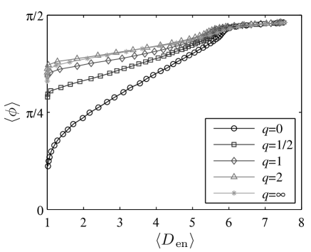
The ensemble and time average angle $\left<\phi\right>$ is shown in Fig. 3, and demonstrates that the logarithmic BVs ($q=0$) are able to achieve a considerable degree of alignment with the LV on average, while retaining some degree of diversity. One clearly sees that BVs constructed with norms $q>0$ become strongly aligned among themselves while still keep a high degree of transversality with the main LV, as reflected by the high average angle of the ensembles ($\left<\phi\right>>\pi/4$) in Fig. 3 for $\left<D_{\mathrm{en}}\right>=1$. In contrast, the ‘logarithmic ensemble’ ($q=0$) exhibits a lower angle with the main LV, even if the statistical diversity is high. We claim that the higher diversity and lower $\left<\phi\right>$ exhibited by the ensemble of logarithmic BVs ($q=0$), as compared with the ensembles with $q>0$, indicates that this ensemble is spanning a sub-space formed by a narrow hyper-cone around the main LV, while ensembles with $q>0$ tend to lie in a lower dimension subspace that is more transverse to the LV.

Figure 3: Average angle between the BVs and the main LV.

V.4 Average growth rate

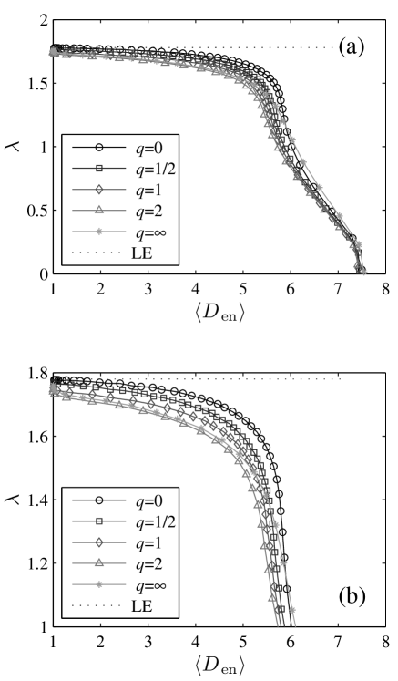
Also the growth rate of the ensemble members can be used to compare with that of the main LV, reflecting again the different behavior for different norm choices. The average exponential growth rate of the bred vectors is

$$\lambda=\frac{1}{T}\left<\ln\left(\frac{\|\mathbf{\Delta u}(t_{m}+T)\|_{2}}{\|\mathbf{b}_{q}(t_{m})\|_{2}}\right)\right>$$ (12)

Notice that, for the sake of clarity we are using the same norm type ($q=2$) to measure the exponential growth rate in all cases (nevertheless due to the long averaging the norm type is irrelevant).

Figure 4 shows the dependence of $\lambda$ on the ensemble dimension. One can see that the logarithmic BVs ($q=0$) exhibit the largest amplification rate for a given ensemble dimension, which is in agreement with the results discussed in the preceding subsections showing that the logarithmic ensemble ($q=0$), among all ensemble choices, exhibited the greatest projection on the LV. Conversely, given an exponential growth rate $\lambda$, using the $0$-norm will result in the most diverse ensemble.

Figure 4: (a) Average growth rate $\lambda$ as a function of the average ensemble dimension. The dotted line indicates the value of the Lyapunov exponent. (b) Zoom of panel (a).

VI Conclusions

We have studied the effect of different norms on the construction of ensembles of BVs. The geometric ($q=0$) norm outperforms other norms (like the Euclidean one, $q=2$) for constructing ensembles of BVs in spatially extended systems. The enhancement of performance (in terms of root-mean square error, ensemble spread, and calibration time) of ensembles of logarithmic ($q=0$) bred vectors with respect to standard “Euclidean” ($q=2$) bred vectors was already uncovered by Primo et al. (2008). In the present work we give a rationale behind those results. We show that an ensemble of logarithmic BVs (obtained with the 0-norm) exhibits greater diversity —larger ensemble dimension— while its members are more strongly projected on the leading LV and have growth rates that rapidly approach the leading Lyapunov exponent. In comparison, ensembles based on BVs with $q>0$ perform rather poorly. They tend to collapse in one single direction (i.e., $\left<D_{\mathrm{en}}\right>=1$) very abruptly as the BV amplitude is diminished and, even when all the statistical diversity is lost, they remain rather transverse to the leading LV as demonstrated by the angle with the main LV shown in Fig. 3. Moreover, the geometric norm also leads to the least fluctuating ensemble dimension among all the possible $q$-norms.

In the view of these results two prominent questions remain open. On the one hand, it would be very interesting to evaluate the performance of $0$-norm BVs in real applications. The study by Primo et al. (2008) of 0-norm BVs already showed promissing, albeit preliminary, results. Clearly, more research is needed in this direction. On the other hand, there is the problem of analyzing the potential advantages of ensemble Kalman filters based on $0$-norm BVs. Our results show that logarithmic BVs have very nice properties regarding statistical diversity, growth rates, and projection onto the main LV. Therefore, a natural question that arises is: to what extent can these features translate into a better performance of ensemble Kalman filtering methods?. We believe our results may serve as a basis for future research along these lines.

D.P. acknowledges support by CSIC under the Junta de Ampliación de Estudios Programme (JAE-Doc). Financial support from the Ministerio de Ciencia e Innovación (Spain) under Projects No. FIS2009-12964-C05-05 and No. CGL2010-21869/CLI is acknowledged.

References

- Anderson (2001) Anderson, J. L., 2001: An ensemble adjustment Kalman filter for data assimilation. Mon. Wea. Rev., 129, 2884–2903.
- Annan (2004) Annan, J. D., 2004: On the orthogonality of bred vectors. Mon. Wea. Rev., 132, 843–849.
- Bishop and Toth (1999) Bishop, C. H. and Z. Toth, 1999: Ensemble transformation and adaptive observations. J. Atmos. Sci., 56, 1748–1765.
- Bretherton et al. (1999) Bretherton, C. S., M. Widmann, V. P. Dymnikov, J. M. Wallace, and I. Bladé, 1999: The effective number of spatial degrees of freedom of a time-varying field. J. Climate, 12, 1990–2009.
- Corazza et al. (2003) Corazza, M., et al., 2003: Use of the breeding technique to estimate the estructure of the analysis ”errors of the day”. Nonlin. Processes Geophys., 10, 233–243.
- Gneiting and Raftery (2005) Gneiting, T. and A. E. Raftery, 2005: Weather forecasting with ensemble methods. Science, 310, 248–249.
- Hallerberg et al. (2010) Hallerberg, S., D. Pazó, J. M. López, and M. A. Rodríguez, 2010: Logarithmic bred vectors in spatiotemporal chaos: Structure and growth. Phys. Rev. E, 81, 066 204.
- Kalnay (2002) Kalnay, E., 2002: Atmospheric Modeling, Data Assimilation and Predictability. Cambridge University Press, Cambridge.
- Kalnay et al. (2002) Kalnay, E., M. Corazza, and M. Cai, 2002: Are bred vectors the same as Lyapunov vectors? AMS Sympos. on observations, data assimilation and probabilistic prediction, 173–177.
- Keller et al. (2010) Keller, J. D., A. Hense, L. Kornblueh, and A. Rhodin, 2010: On the orthogonalization of bred vectors. Wea. and Forecasting, 25, 1219–1234.
- Lorenz (1996) Lorenz, E. N., 1996: Predictability a problem partly solved. Proc. Seminar on Predictability Vol. I, T. Palmer, Ed., ECMWF, Reading, UK, ECWF Seminar, 1–18.
- Lorenz (2006) Lorenz, E. N., 2006: Regimes in simple systems. J. Atmos. Sci., 63, 2056–2073.
- Lorenz and Emanuel (1998) Lorenz, E. N. and K. A. Emanuel, 1998: Optimal sites for suplimentary weather observations: Simulations with a small model. J. Atmos. Sci., 55, 399–414.
- Newman et al. (2004) Newman, C. E., P. L. Read, and S. R. Lewis, 2004: Investigating atmospheric predictability on Mars using breeding vectors in a general-circulation model. Q. J. R. Meteorol. Soc., 130, 2971–2989.
- Oczkowki et al. (2005) Oczkowki, M., I. Szunyogh, and D. J. Patil, 2005: Mechanisms for the development of locally low-dimensional atmospheric dynamics. J. Atmos. Sci., 62, 1135–1156.
- Patil et al. (2001) Patil, D. J., B. R. Hunt, E. Kalnay, J. A. Yorke, and E. Ott, 2001: Local low dimensionality of atmospheric dynamics. Phys. Rev. Lett., 86, 5878–5881.
- Pazó et al. (2010) Pazó, D., M. A. Rodríguez, and J. M. López, 2010: Spatio-temporal evolution of perturbations in ensembles initialized by bred, Lyapunov and singular vectors. Tellus, 62A, 10–23.
- Primo et al. (2008) Primo, C., M. A. Rodríguez, and J. M. Gutiérrez, 2008: Logarithmic bred vectors. A new ensemble method with adjustable spread and calibration time. J. Geophys. Res., 113, D05 116.
- Primo et al. (2005) Primo, C., M. A. Rodríguez, J. M. López, and I. Szendro, 2005: Predictability, bred vectors, and generation of ensembles in space-time chaotic systems. Phys. Rev. E, 72, 015 201.
- Primo et al. (2006) Primo, C., I. G. Szendro, M. A. Rodríguez, and J. M. López, 2006: Dynamic scaling of bred vectors in spatially extended chaotic systems. Europhys. Lett., 76, 767–773.
- Toth and Kalnay (1993) Toth, Z. and E. Kalnay, 1993: Ensemble forecasting at NMC: the generation of perturbations. Bull. Amer. Meteor. Soc., 74, 2317–2330.
- Toth and Kalnay (1997) Toth, Z. and E. Kalnay, 1997: Ensemble forecasting at NCEP: the breeding method. Mon. Wea. Rev., 125, 3297–3318.
- Wang and Bishop (2003) Wang, X. and C. Bishop, 2003: A comparison of breeding and ensemble transform Kalman filter ensemble forecast schemes. J. Atmos. Sci., 60, 1140–1158.
- Wei et al. (2008) Wei, M., Z. Toth, R. Wobus, and Y. Zhu, 2008: Initial perturbations based on the ensemble transform (ET) technique in the NCEP global operational forecast system. Tellus, 60A, 62–79.
- Wei et al. (2006) Wei, M., Z. Toth, R. Wobus, Y. Zhu, C. Bishop, and X. Wang, 2006: Ensemble transform kalman filter-based ensemble perturbations in an operational global prediction system at ncep. Tellus, 58A, 1–28.
- Young and Read (2008) Young, R. M. B. and P. L. Read, 2008: Breeding and predictability in the baroclinic rotating annulus using a perfect model. Nonlin. Processes Geophys., 15, 469–487.