Bistable collective behavior of polymers tethered in a nanopore

Abstract

Polymer-coated pores play a crucial role in nucleo-cytoplasmic transport and in a number of biomimetic and nanotechnological applications. Here we present Monte Carlo and Density Functional Theory approaches to identify different collective phases of end-grafted polymers in a nanopore and to study their relative stability as a function of intermolecular interactions. Over a range of system parameters that is relevant for nuclear pore complexes, we observe two distinct phases: one with the bulk of the polymers condensed at the wall of the pore, and the other with the polymers condensed along its central axis. The relative stability of these two phases depends on the interpolymer interactions. The existence the two phases suggests a mechanism in which marginal changes in these interactions, possibly induced by nuclear transport receptors, cause the pore to transform between open and closed configurations, which will influence transport through the pore.

I Introduction

Physical modeling is a powerful tool to interpret the complexity arising from multiple interacting components in a biological system. One such system is the nuclear pore complex (NPC). This structure mediates all transport between the cell cytoplasm and the nucleus, and its operation is thought to depend on the properties of natively unfolded proteins, nucleoporins, that are end-grafted inside a $\sim$50 nm wide channel Peters (2009); Wente and Rout (2010); Jamali et al. (2011); Hoelz et al. (2011). Molecules larger than $\sim$6 nm can only pass through this nanopore if they are bound to nuclear transport receptors, which are known to interact with the nucleoporins. Though the composition, hydrodynamic size, and nanomechanical properties of single nucleoporins are known in great detail Hoelz et al. (2011); Yamada et al. (2010); Lim et al. (2006), their collective behavior in the NPC is still heavily disputed. This behavior has been studied using a variety of models, with nucleoporins in a one-dimensional geometry Zilman et al. (2007), grafted to a planar surface Miao and Schulten (2009) and constrained within a rectangular box Kustanovich and Rabin (2004). Only very recently has the cylindrical geometry of the pore been taken into account Peleg and Lim (2010); Moussavi-Baygi et al. (2011); Mincer and Simon (2011); Egorov et al. (2011).

More generally, there has been significant interest in polymer coatings in nanopores, since they can be used to tune the aperture of artificial and biomimetic nanopores and filters Iwata et al. (1998); Wanunu and Meller (2007); Yameen et al. (2009); Lim and Deng (2009); Jovanovic-Talisman et al. (2009); Kowalczyk et al. (2011). Polymers end-grafted in a cylindrical pore have been studied by molecular dynamics Adiga and Brenner (2005) and Monte Carlo Koutsioubas et al. (2009) simulations. Depending on solvent quality, pore diameter and polymer structure and dimensions, there can be a rich and complex phase diagram Dimitrov et al. (2006); Wang et al. (2010); Peleg et al. (2011).

In this paper, we investigate the effect of confinement on the possible conformations of polymers within a cylindrical channel. We have performed Monte Carlo simulations on a coarse-grained model of polymers end-grafted within a cylinder, and have furthermore developed an approach using density functional theory (DFT) to study the relative stability of competing morphologies. The DFT free energy is based on a reference case of a tethered freely jointed chain of point-like beads, a novel choice in this context, and its mean field variational optimization has been carried out using a highly efficient numerical procedure. The resulting well-founded free energy estimates enable us to construct a phase diagram indicating the relative stability of different polymer configurations and to speculate about transitions that might be induced between them.

Figure 1: (Color online) (a) Illustration of the polymer model where bead $n$ is constrained to lie on a circle such that the length of the bonds to beads $n-1$ and $n+1$ is unchanged. (b) Snapshot of a Monte Carlo simulation with 40 non-interacting polymers of contour length 100 nm, bead diameter $d=1$ nm and bond length $b=1$ nm, end-grafted to the thick dots in a cylindrical pore of 25 nm radius.

II Models of nucleoporin behavior

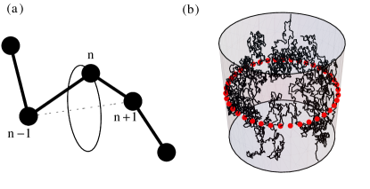
Nucleoporins in the NPC channel have been shown to separate into two distinct categories: those that form short globular conformations, and longer polymers that tend to be able to extend further away from their tethering point at the NPC rim Yamada et al. (2010). As cylindrical confinement will mostly affect those nucleoporins with contour length much greater than the pore radius, we focus on this latter category: polymers with  100 nm contour length, end-grafted on a ring around the inner wall of a long cylinder with a radius $R=25$ nm (Fig. 1). We model the polymers as freely jointed chains of beads of diameter $d=1$ nm, with a segment length $b=1$ nm. This implies a persistence length of 0.5 nm, in agreement with single-molecule pulling experiments on nucleoporin cNup153 Lim et al. (2006). Excluded-volume effects are modeled as a hard-sphere repulsion between the beads. They are supplemented by longer-ranged attractive interactions between the polymers, consistent with those that appear to operate in the NPC Peters (2009); Wente and Rout (2010); Jamali et al. (2011); Hoelz et al. (2011). The combined bead-bead pair potential therefore takes the form

$$\phi(\mathbf{r})=\begin{cases}\infty&|\mathbf{r}|<d\\ -\epsilon\exp[-(|\mathbf{r}|-d)/\lambda]&|\mathbf{r}|\geq d\,,\end{cases}$$ (1)

where $\mathbf{r}$ is the vector connecting the centers of the beads, and $\lambda$ and $\epsilon$ are range and strength parameters, respectively. A variety of interaction mechanisms might be represented by an appropriate choice of $d$, $\lambda$ and $\epsilon$ in Eq.  (1), including, for example, the hydrophobic interaction that is thought to play a significant role in these systems Israelachvili (2011).

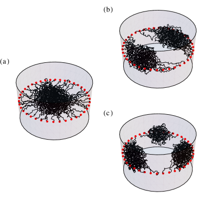
As a first approach to determine typical polymer configurations, we study the system by Monte Carlo (MC) simulations. We employ a straightforward Metropolis algorithm, in which single beads attempt moves on a circular path defined by the constant distance $b$ to their nearest neighbors, whilst remaining restricted to the inner volume of the cylinder as illustrated in Fig. 1. The first bead for each polymer, located on the cylinder inner surface, is fixed in position, whilst the last bead is free to move on the surface of the sphere of radius $b$ centered on the penultimate bead. The restriction of constant segment length simplifies the description of each MC move, but can slow down the exploration of configuration space. Nevertheless, all polymer conformations are accessible from one another. We perform simulations of 250000 attempted moves per bead. Relaxation to equilibrium is confirmed by noting convergence of the system energy, such that we use the second half of each simulation to generate mean bead profiles. The simulations indicate an interesting range of behavior, as can be seen in Fig. 2 for 40 polymers, each of length 100 beads, tethered uniformly around a ring. Different dominant configurations may be observed depending on the parameters chosen, though they can be roughly divided into two categories: conformations in which the density is peaked in the center, and those in which it is peaked closer to the wall. Sometimes profiles from both categories emerge even for the same parameter choice, depending on the starting configuration. This suggests that there exist thermodynamically stable and metastable states for a particular parameter set.

Figure 2: (Color online) Snapshots taken from converged Monte Carlo simulations as in Fig. 1, showing different results for polymers that are subject to the same excluded volume and attractive interactions, as defined by Eq. 1 with $\epsilon=0.1\,k_{B}T$ and $\lambda=1.0$ nm. (a): Condensation in the center. (b) and (c): Different numbers of clumps can be found when the polymers condense closer to the wall.

In order to categorize these phases more fully, and in particular to investigate the relative stability of wall and central configurations, a variational mean field density functional theory (DFT) of a many-polymer system has been developed. DFT provides a natural framework for evaluating the free energy of large numbers of interacting particles Evans (1979), though certain modifications are necessary for it to be suitable as a model of a system of polymers. It shares many of the features of a self-consistent statistical field theory of polymers Frederikson (2006), and has the capacity to include finite-range interactions, as expressed in the pair-potential $\phi(\mathbf{r})$. The polymer entropy is estimated by solving an equivalent Brownian motion problem, in contrast to other approaches that are also based on the minimization of a free energy functional but estimate the entropy by numerically generating a large set of sample configurations Peleg et al. (2011). Our model can be implemented using an efficient numerical algorithm that runs on a standard desktop PC. It can be used to explore the equilibrium behaviour of the system. Dynamical versions of DFT have been developed to include relaxational phenomena Marconi and Tarazona (1999); Marconi and Melchionna (2007), and our model has the potential to be extended in this direction.

The DFT model applied to a single chain of $N$ beads employs the Hamiltonian

$$H=\sum_{i=0}^{N-1}h(\mathbf{r}_{i+1},\mathbf{r}_{i})+\frac{1}{2}\sum_{j=0}^{N}\sum_{i\neq j}^{N}\phi(\mathbf{r}_{i}-\mathbf{r}_{j})\,,$$ (2)

where $\mathbf{r}_{i}$ is the position of bead $i$, $h$ is a function that constrains each segment of the polymer chain to take a fixed length $b$, and the potential $\phi$ acts between all pairs of beads. In the variational mean field approach, we introduce an additional potential $V$ such that $H=H_{0}+H_{1}$ with

$$H_{0} = \sum_{i=0}^{N-1}h(\mathbf{r}_{i+1},\mathbf{r}_{i})+\sum_{i=1}^{N}V(\mathbf{r}_{i})$$ (3)

$$H_{1} = \frac{1}{2}\sum_{j=0}^{N}\sum_{i\neq j}^{N}\phi(\mathbf{r}_{i}-\mathbf{r}_{j})-\sum_{i=1}^{N}V(\mathbf{r}_{i})\,.$$ (4)

$H_{0}$ describes a chain of $N$ point-like beads interacting with an external potential $V$, constrained by a requirement of constant segment length, and with the first bead coupled to a static tethering point at $\mathbf{r}_{0}$. This system has thermodynamic properties embodied in the free energy Frederikson (2006)

$$F_{0}=-\ln\left(\int G(\mathbf{r}_{0},\mathbf{r},N;[w])\mathrm{d}\mathbf{r}\right)\,,$$ (5)

in units of $k_{B}T$, where $G(\mathbf{r}_{0},\mathbf{r},N;[w])$ is the propagator of a Brownian motion with contour length $Nb$ from tether point $\mathbf{r_{0}}$ to point $\mathbf{r}$ inside the cylinder, evolving under the influence of a dimensionless external potential $w(\mathbf{r})=V(\mathbf{r})/k_{B}T$ acting as a sink; namely the Green’s function solution Doi and Edwards (1986) to the diffusive problem described by

$$\frac{\partial G(\mathbf{r}_{0},\mathbf{r},s;[w])}{\partial s}=\left(\frac{b^{2}}{6}\nabla^{2}-w(\mathbf{r})\right)G(\mathbf{r}_{0},\mathbf{r},s;[w])$$ (6)

with initial condition $G=\delta(\mathbf{r}-\mathbf{r}_{0})$ at $s=0$, and boundary conditions $G=0$ at the cylinder wall and zero radial gradient at the center. $\rho(\mathbf{r})$ is the single bead distribution function evaluated for the Hamiltonian $H_{0}$; it is a functional of $w$, and is given in terms of $G$ as Doi and Edwards (1986)

$$\!\rho(\mathbf{r})\!=\frac{\int_{0}^{N}\!\mathrm{d}s\int\!\mathrm{d}\mathbf{r^{\prime}}G(\mathbf{r}_{0},\mathbf{r},N-s;[w])G(\mathbf{r},\mathbf{r^{\prime}},s;[w])}{\int\mathrm{d}\mathbf{r^{\prime}}G(\mathbf{r}_{0},\mathbf{r^{\prime}},N;[w])}.$$ (7)

It is important to recognise that the mean field in DFT is a single-bead potential that is introduced to emulate the real polymer self-interactions as closely as possible. The reference Hamiltonian $H_{0}$ describes the behavior of $N$ freely jointed beads in the potential $V$, and the absence of additional bead-bead interactions simplifies its analysis considerably. The DFT-derived bead density profiles represent polymer configurations adopted in response to a mean field potential instead of the actual self-interactions. This can be a reasonable approximation if the mean field is optimized, as can be recognized through use of the Bogoliubov inequality. Within such an approach, the best description of the interacting polymer system can be obtained by minimizing the free energy

$$F_{{\rm mf}}\!=\!F_{0}-\!\int\!\!\rho(\mathbf{r})w(\mathbf{r})\mathrm{d}\mathbf{r}+F_{{\rm hc}}+\frac{1}{2}\!\int\!\!\rho(\mathbf{r})\rho(\mathbf{r^{\prime}})u(\mathbf{r}-\mathbf{r^{\prime}})\mathrm{d}\mathbf{r}\mathrm{d}\mathbf{r^{\prime}}$$ (8)

with respect to the mean field $w$, bearing in mind that $\rho$ depends on $w$. Both $F_{{\rm mf}}$ and $u$, the attractive part of the bead pair potential $\phi$, are expressed in units of $k_{B}T$. The contribution to the free energy arising from the attractive term is derived on the basis of a random phase approximation. The contribution from the repulsive interactions is modeled by a hard chain free energy $F_{{\rm hc}}$ described in the local density approximation, and in units of $k_{B}T$, by Wertheim (1987); Egorov (2008):

$$F_{{\rm hc}}= \int\rho(\mathbf{r})\left[\frac{4\eta(\mathbf{r})-3\eta(\mathbf{r})^{2}}{[1-\eta(\mathbf{r})]^{2}}-\right.$$ (9)

$$\left.\left(1-\frac{1}{N}\right)\ln\left(\frac{2-\eta(\mathbf{r})}{2[1-\eta(\mathbf{r})]^{3}}\right)\right]\,\mathrm{d}\mathbf{r}$$

where $\eta(\mathbf{r})$ is a bead packing fraction given by $\pi\rho(\mathbf{r})d^{3}/6$. The origin of Eq. (8) is described in detail in Appendix A.

The model so far has been constructed for a single polymer, but a system of $M$ polymers in a pore can be treated by multiplying $F_{0}$ by $M$, by interpreting $\rho$ in the remaining terms in Eq. (8) as the superposition of bead density profiles of the $M$ polymers attached to their separate tether points, and by regarding the entire free energy $F_{{\rm mf}}$ as a functional of a mean field $w$ that we assume, for simplicity, to exhibit the cylindrical symmetry of the pore.

Figure 3: (Color Online) Mean bead density profiles for Monte Carlo (MC) simulations (a) and DFT calculations (b) for 40 polymers, composed of 100 beads each, tethered within a cylinder, and interacting only through hard sphere interactions. The plots are given for a range of radial ($r$) and axial ($z$) coordinates. (c) and (d) show more detailed comparisons of the profiles as a function of, respectively, the radial direction in the plane of the tethering ring ($z=0$), and the axial direction at a radius $r=17.5$ nm. DFT results are given by the solid lines and the statistical uncertainty in the MC results is indicated with error bars.

We minimize the free energy functional (8) using a conjugate gradient method (Polak-Ribiere) Press (2007); Frederikson (2006), on the basis of gradient information obtained by evaluating the functional derivative $\delta F_{{\rm mf}}\left[\rho\right]/\delta\rho$. This has proved to be more efficient in this context than employing the gradient information within a steepest descent method: this is discussed in greater detail in Appendix A. The numerical scheme involves making an initial guess for $w(\mathbf{r})$, evaluating the bead density using Eq. (7), thereby obtaining the mean field free energy through Eq. (8) and using the conjugate gradient scheme to generate a new free energy, and hence a new mean field. The mean field and the bead density are defined numerically on a grid of points within the cylinder, fine enough such that the spacing does not affect the outcome of the calculations.

III Comparison between MC and DFT

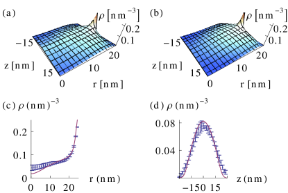
A key test of the DFT model, and of the numerical scheme, is to compare bead density profiles with those obtained by MC simulation. We look first at polymers interacting only through hard sphere repulsion, represented in the DFT by the contribution in Eq. (9). The comparison shown in Fig. 3 shows a good agreement between the two schemes, indicating that the DFT approach captures the essence of the excluded volume behavior.

Figure 4: (Color online) Converged polymer configurations and bead density profiles calculated for an attractive pair potential of depth $\epsilon=0.1\,k_{B}T$ and range $\lambda=1.0$ nm in a pore of 25 nm radius. The data in the left and right column correspond to initial conditions with the 40 polymers concentrated at the wall and at the center, respectively. (a-b) DFT results with parameters corresponding to the Monte Carlo simulations, as a function of radial ($r$) and axial ($z$) position. (c-d) Comparison of Monte Carlo (with error bars) and DFT (smooth curves) radial profiles for $z=0$, the plane of the tethering points. Axial profiles (e) for the wall phase at $r=22.5$ nm and (f) for the central phase at $r=2.5$ nm.

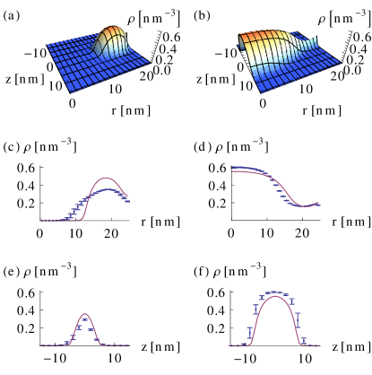
Next, we include long range interactions and make a similar comparison between DFT and MC results. This test is more challenging since there is now competition between polymer attraction and repulsion, giving rise to quite distinct configurations, as we saw earlier for the MC alone. Whilst the DFT can treat cases with different radial density profiles, it presently does not explicitly allow for azimuthal clumping. Fig. 4(a-b) illustrates two converged density profiles obtained from the DFT approach, arising from different choices for the initial mean field. They are the counterparts to the wall and central phases observed in Monte Carlo simulations seen in Fig. 2, and use the same set of interaction parameters, namely $\epsilon=0.1\,k_{B}T$ and $\lambda=1.0$ nm. A detailed comparison of the centrally peaked profiles with MC results in Figs. 4(d) and (f) suggests that the radial and axial spread of the polymers determined from each approach are consistent with one another. For the wall phase, the DFT and MC profiles do differ, as illustrated radially and axially in Figs. 4(c) and (e). The differences might be due to the angular symmetry breaking, or clumping, observed in the Monte Carlo simulations, but this would not be expected to affect the qualitative conclusions about the stability or metastability of the two phases that we now explore.

The great benefit of the DFT model is that it provides thermodynamic properties of the interacting polymers within the pore, not just the structural properties that are available using MC. It provides estimates of the free energy, such that it is possible to determine which phase, central or wall, is thermodynamically stable or metastable under a range of interaction conditions.

Figure 5: (Color online) Metastability diagram of the polymer phases as a function of strength $\epsilon$ and range $\lambda$ of the attractive interactions. $\Delta F_{\mathrm{p}}$ indicates the free energy difference per polymer between the wall and central phases, for parameters where they can both exist as a stable and metastable state. The coexistence conditions lie along the boundary between blue and red regions. In the green region, only one phase is found to be possible: the metastability of the other has been lost.

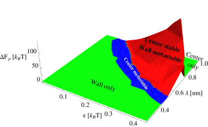
In Fig. 5 we plot the difference in free energy between wall and central profiles $\Delta F_{\mathrm{p}}$, per polymer and in units of $k_{B}T$, against interaction range $\lambda$ and strength $\epsilon$. The plot illustrates the free energy difference as a surface extending across regions where, respectively, the central phase (‘Center stable, wall metastable’) and the wall phase (‘Center metastable’) are thermodynamically stable and the other phase is metastable. The region in the foreground (‘Wall only’) denotes conditions where only the wall phase appears to exist. Similarly, there is a corresponding region where only the central phase exists towards the back of the diagram (‘Center only’). There is a binodal line, or phase boundary, where wall and central phase coexist, together with spinodals denoting the extremes of metastability of one of the phases with respect to the other. When we extend the range of $\epsilon$ to larger values, i.e. stronger attractions than those shown, we find that the phase boundary continues in such a manner such that a central phase is increasingly favored.

The metastability diagram demonstrates that central polymer condensation is a natural result of attractive interactions, provided that their range and strength are sufficiently large. This is in accord with intuition, which suggests that a central phase can be stabilized by a reduction in energy to balance the cost in entropy of extending the polymers away from the wall. A long range attractive potential will favor this by allowing polymers to interact with more of their counterparts across the other side of the pore. If the range were reduced, then the required strength of the attraction would have to be greater to produce the same effect. Repulsive interactions do not drive bistable phase behavior. Instead the polymer condensate becomes more homogeneous as the strength of the repulsion is increased: such behavior is equivalent to that of a good solvent.

Figure 6: Free energies of the central phases (solid) and wall phases (dashed) for systems with a range of bead number $N$, per polymer, for interaction range $\lambda=0.5$ nm, plotted as a function of interaction strength $\epsilon$. The phase with the lower free energy is thermodynamically stable. The limited extent of the curve of higher free energy, in some cases, is an illustration of the limits of the metastability of that phase, equivalent to spinodal behavior. As $N$ increases, the central phase becomes stable over a larger range of $\epsilon$.

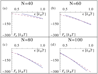
In addition to changing the strength and range of the polymer interactions, we can also explore the effect of a change in the number of beads $N$ in each polymer. For constant segment length $b$, this is equivalent to altering the length of the polymer. Reducing $N$ has the dual effect of increasing the entropic cost of stretching a polymer towards the center of the pore, and of decreasing the binding energy that can be experienced by each polymer. Both effects hinder central phase formation, and this is borne out in calculations of free energies for the two phases as a function of interaction strength $\epsilon$ for a range of $N$, as shown in Fig. 6 for $\lambda=0.5$ nm. Shortening the length of the polymers requires a stronger attractive potential for the polymers to condense towards the pore center, as is to be expected.

IV Discussion and Conclusions

On the basis of Monte Carlo and density functional theory calculations, we find that polymers tethered around a ring inside a cylindrical geometry can exhibit bistable behavior, switching between a wall- and a centrally condensed phase depending on the interaction parameters. Interestingly, this behavior is observed for a geometry and polymer structural properties that closely resemble the NPC Peters (2009); Wente and Rout (2010); Jamali et al. (2011); Hoelz et al. (2011), for entirely realistic ranges ($\lambda\lesssim 1$ nm) and strengths ($\epsilon\lesssim 1\,k_{B}T$) of intermolecular interactions Israelachvili (2011) within the NPC. The existence of a central polymer condensate is reminiscent of the central ‘plug’ or ‘transporter’ structure of nucleoporins that has been observed by cryo-electron microscopy of the nuclear pore complex (NPC) Hoelz et al. (2011); Yamada et al. (2010), though our model would need to be developed to treat a more realistic geometry if it were to be considered a proper representation. Nevertheless, our thermodynamic model suggests that a phase transition from the central to the wall phase occurs when the effective strength or range of the attraction between polymer segments is decreased. Equivalently, the transition might be induced by increasing the prevailing temperature. If we were to apply our model to the NPC, this feature would be in agreement with the experimentally observed dissolution of the central plug at higher temperature Stoffler et al. (2003). A similar effect has been seen upon incubation of the NPC with nuclear transport receptors Kramer et al. . A possible interpretation of this effect is that the nuclear transport receptors are responsible for a weakening of the nucleoporin self-attraction and that their influence on the polymer plug provides a mechanism for the differential permeability of the NPC. In this scenario, a sufficiently high concentration of nuclear transport receptors disturbs the thermodynamic stability of the central structure to the extent that the polymers withdraw towards the wall, leaving a free passage to be occupied and traversed by receptors and receptor-bound cargos. Such a mechanism, if it operates, could be exploited in the design of artificial nanopores that might perform similar differential transport of a variety of molecular species.

Appendix A Details of the free energy functional

We provide here some theoretical and numerical background, including a detailed specification of the bead density profile, the rationale for the variational principle employed, and the condition for minimizing the free energy using functional derivatives. We focus our interest on the statistical properties of a Hamiltonian $H_{0}$ for a freely jointed polymer of $N$ point-like beads at positions $\{\mathbf{r}_{i}\}$ in a dimensionless external potential $w$, given by $H_{0}=U\left(\left\{\mathbf{r}_{i}\right\}\right)+k_{B}T\sum_{i=1}^{N}w(\mathbf{r}_{i})$, where $U\left(\left\{\mathbf{r}_{i}\right\}\right)=\sum_{i}h(\mathbf{r}_{i+1},\mathbf{r}_{i})$ is a function that imposes the constraints on bond length. The bead at $\mathbf{r}_{1}$ is constrained with respect to the tether point at $\mathbf{r}_{0}$. The partition function of the system is

$$Z_{0}=\int\prod_{j=1}^{N}\mathrm{d}\mathbf{r}_{j}\exp\left[-U/k_{B}T-\sum_{i=1}^{N}w(\mathbf{r}_{i})\right].$$ (10)

The configuration-dependent bead density over continuous spatial position $\mathbf{r}$ is defined as $\hat{\rho}(\mathbf{r},\left\{\mathbf{r}_{k}\right\})=\sum_{i=1}^{N}\delta(\mathbf{r}-\mathbf{r}_{i})$, which allows us to write $Z_{0}$ as

$$Z_{0}[w]=\!\int[\mathrm{d}\mathbf{r}_{i}]\exp\left(-U/k_{B}T-\!\int\!\hat{\rho}(\mathbf{r})w(\mathbf{r})\mathrm{d}\mathbf{r}\right),$$ (11)

where $[\mathrm{d}\mathbf{r}_{i}]$ represents the integration over bead positions and we compress the notation of $\hat{\rho}$ for clarity.

The partition function is clearly a functional of the external potential $w$ and its functional derivative is:

$$\frac{\delta Z_{0}[w]}{\delta w(\mathbf{y})}=$$ (12)

$$\lim_{\epsilon\to 0}\frac{1}{\epsilon}\!\left[\int\![\mathrm{d}\mathbf{r}_{i}]\exp\!\left(\!-\frac{U}{k_{B}T}-\!\int\!\!\hat{\rho}(\mathbf{r})\!\left(w(\mathbf{r})\!+\!\epsilon\delta(\mathbf{r}-\mathbf{y})\right)\!\mathrm{d}\mathbf{r}\!\right)\right.$$

$$\left.-\int[\mathrm{d}\mathbf{r}_{i}]\exp\left(-\frac{U}{k_{B}T}-\int\hat{\rho}(\mathbf{r})w(\mathbf{r})\,\mathrm{d}\mathbf{r}\right)\right]$$

$$=-\int[\mathrm{d}\mathbf{r}_{i}]\hat{\rho}(\mathbf{y})\exp\left(-U/k_{B}T-\int\hat{\rho}(\mathbf{r})w(\mathbf{r})\,\mathrm{d}\mathbf{r}\right),$$

such that we can define $\rho(\mathbf{y})=\langle\hat{\rho}(\mathbf{y})\rangle$ to be the mean bead density for the system:

$$\rho(\mathbf{y}) =\frac{1}{Z_{0}}\int[\mathrm{d}\mathbf{r}_{i}]\hat{\rho}(\mathbf{y})\exp\left(-U/k_{B}T-\int\hat{\rho}(\mathbf{r})w(\mathbf{r})\,\mathrm{d}\mathbf{r}\right)$$ (13)

$$=-\frac{1}{Z_{0}[w]}\frac{\delta Z_{0}[w]}{\delta w(\mathbf{y})}=-\frac{\delta\ln Z_{0}[w]}{\delta w(\mathbf{y})},$$

which demonstrates that $\rho$ is a functional of $w$. The explicit functional dependence is given in Eq. (7).

Now we discuss a self-interacting polymer described by the Hamiltonian

$$H=U+\frac{1}{2}\sum_{j=1}^{N}\sum_{i\neq j}^{N}\phi(\mathbf{r}_{i}-\mathbf{r}_{j})\,,$$ (14)

incorporating a potential $\phi$ acting between all bead pairs. We write $H=H_{0}+H_{1}$ with

$$H_{1}=\frac{1}{2}\sum_{j=1}^{N}\sum_{i\neq j}^{N}\phi(\mathbf{r}_{i}-\mathbf{r}_{j})-k_{B}T\sum_{i=1}^{N}w(\mathbf{r}_{i})\,,$$ (15)

and employ the Bogoliubov inequality $F\leq F_{0}+\langle H_{1}\rangle$, where $F$ is the free energy of the system described by Hamiltonian $H$, and $F_{0}=-\ln Z_{0}$ is the free energy of the reference system described by $H_{0}$, in units of $k_{B}T$, and is given by Eq. (5) Frederikson (2006). As before, the brackets denote an average over the ensemble associated with $H_{0}$, and we write

$$\left\langle\sum_{i=1}^{N}w(\mathbf{r}_{i})\right\rangle=$$ (16)

$$\frac{1}{Z_{0}}\int[\mathrm{d}\mathbf{r}_{i}]\!\int\!\hat{\rho}(\mathbf{y})w(\mathbf{y})\,\mathrm{d}\mathbf{y}\exp\left(-\frac{U}{k_{B}T}-\!\int\!\hat{\rho}(\mathbf{r})w(\mathbf{r})\,\mathrm{d}\mathbf{r}\!\right)$$

$$=\int\rho(\mathbf{y})w(\mathbf{y})\,\mathrm{d}\mathbf{y}.$$

In a similar fashion the mean of the pairwise terms is

$$\!\!\left\langle\sum_{j=1}^{N}\sum_{i\neq j}^{N}\phi(\mathbf{r}_{i}-\mathbf{r}_{j})\right\rangle=$$ (17)

$$\!\frac{1}{Z_{0}}\!\int\![\mathrm{d}\mathbf{r}_{i}]\!\!\int\!\!\hat{\rho}_{2}(\mathbf{x},\mathbf{y},\left\{\mathbf{r}_{k}\right\})\phi(\mathbf{x}\!-\!\mathbf{y})\mathrm{\mathrm{d}\mathbf{x}d}\mathbf{y}$$

$$\!\!\times\!\exp\!\left(\!\!-\frac{U}{k_{B}T}-\!\!\int\!\!\hat{\rho}(\mathbf{r})w(\mathbf{r})\mathrm{d}\mathbf{r}\!\right)\!=\!\!\int\!\!\rho_{2}(\mathbf{x},\mathbf{y})\phi(\mathbf{x}-\mathbf{y})\mathrm{d}\mathbf{x}\mathrm{d}\mathbf{y},$$

where $\hat{\rho}_{2}(\mathbf{x},\mathbf{y},\left\{\mathbf{r}_{k}\right\})=\sum_{i\neq j}\delta(\mathbf{x}-\mathbf{r}_{i})\delta(\mathbf{y}-\mathbf{r}_{j})$ is the two-point configuration-dependent bead distribution and $\rho_{2}(\mathbf{x},\mathbf{y})=\langle\hat{\rho}_{2}(\mathbf{x},\mathbf{y},\left\{\mathbf{r}_{k}\right\})\rangle$ is its mean in the $H_{0}$ ensemble. For simplicity, we take a random phase approximation and represent $\rho_{2}(\mathbf{x},\mathbf{y})$ by $\rho(\mathbf{x})\rho(\mathbf{y})$. Thus the free energy of the self-interacting polymer is bounded by the inequality

$$F\!\leq\!-\ln Z_{0}[w]-\!\int\!\!\rho(\mathbf{y})w(\mathbf{y})\mathrm{d}\mathbf{y}+\frac{1}{2}\!\int\!\!\rho(\mathbf{x})\rho(\mathbf{y})\bar{\phi}(\mathbf{x}-\mathbf{y})\mathrm{d}\mathbf{x}\mathrm{d}\mathbf{y},$$ (18)

where $\bar{\phi}$ is the pair potential divided by $k_{B}T$, which can be separated into an attractive part $u(\mathbf{x}-\mathbf{y})$ and a repulsive part. The latter’s contribution to the right hand side may be represented by a functional $F_{{\rm hc}}[\rho]$ (Eq. (9)) that has been found to capture the thermodynamic properties of hard chains: freely jointed polymers of finite size hard spheres Wertheim (1987); Egorov (2008). The free energy then satisfies

$$F\leq F_{\mathrm{mf}}[w]=-\ln Z_{0}[w]+F_{{\rm hc}}[\rho]-\int\!\!\rho(\mathbf{y};[w])w(\mathbf{y})\,\mathrm{d}\mathbf{y}$$ (19)

$$+\frac{1}{2}\int\!\rho(\mathbf{x};[w])\rho(\mathbf{y};[w])u(\mathbf{x}-\mathbf{y})\,\mathrm{d}\mathbf{x}\mathrm{d}\mathbf{y},$$

where the functional dependence of $\rho$ on the mean field $w$ is explicitly noted.

The best estimate of $F$ is identified by functional minimization of the mean field formulation $F_{\mathrm{mf}}[w]$ over all possible $w$, to be achieved by setting the functional derivative $\delta F_{\mathrm{mf}}/\delta w(\mathbf{r})$ to zero. Several contributions to the derivative arise. We already have $\delta\ln Z_{0}/\delta w(\mathbf{r})=-\rho(\mathbf{r};[w])$ from Eq. (13), and furthermore, regarding $F_{{\rm hc}}$ as a functional of either $w$ or $\rho$,

$$\frac{\delta F_{{\rm hc}}[w]}{\delta w(\mathbf{r})}=\!\!\int\!\frac{\delta F_{{\rm hc}}[\rho]}{\delta\rho(\mathbf{y})}\frac{\delta\rho(\mathbf{y};[w])}{\delta w(\mathbf{r})}\mathrm{d}\mathbf{y}=\!\!\int\!\!\mu_{{\rm hc}}(\mathbf{y)}\frac{\delta\rho(\mathbf{y};[w])}{\delta w(\mathbf{r})}\mathrm{d}\mathbf{y},$$ (20)

where $\mu_{{\rm hc}}$ represents the functional derivative of $F_{{\rm hc}}$ with respect to $\rho$, together with

$$\frac{\delta}{\delta w(\mathbf{r})}\!\int\!\!\rho(\mathbf{y};[w])w(\mathbf{y})\mathrm{d}\mathbf{y}\!=\rho(\mathbf{r};[w])+\!\int\!\frac{\delta\rho(\mathbf{y};[w])}{\delta w(\mathbf{r})}w(\mathbf{y})\mathrm{d}\mathbf{y}$$ (21)

and

$$\frac{\delta}{\delta w(\mathbf{r})}\int\rho(\mathbf{x};[w])\rho(\mathbf{y};[w])u(\mathbf{x}-\mathbf{y})\mathrm{d}\mathbf{x}\mathrm{d}\mathbf{y}$$ (22)

$$=2\int\frac{\delta\rho(\mathbf{y};[w])}{\delta w(\mathbf{r})}\rho(\mathbf{x};[w])u(\mathbf{x}-\mathbf{y})\mathrm{d}\mathbf{x}\mathrm{d}\mathbf{y},$$

giving the minimization condition as:

$$\frac{\delta F_{\mathrm{mf}}[w]}{\delta w(\mathbf{r})}=-\!\int\!\frac{\delta\rho(\mathbf{y};[w])}{\delta w(\mathbf{r})}w(\mathbf{y})\mathrm{d}\mathbf{y}\!+\!\!\int\!\!\mu_{{\rm hc}}(\mathbf{y)}\frac{\delta\rho(\mathbf{y};[w])}{\delta w(\mathbf{r})}\mathrm{d}\mathbf{y}$$ (23)

$$+\int\frac{\delta\rho(\mathbf{y};[w])}{\delta w(\mathbf{r})}\rho(\mathbf{x};[w])u(\mathbf{x}-\mathbf{y})\,\mathrm{d}\mathbf{x}\mathrm{d}\mathbf{y}=0.$$

Since

$$\frac{\delta F_{\mathrm{mf}}[w]}{\delta w(\mathbf{r})}=\int\frac{\delta F_{\mathrm{mf}}[\rho]}{\delta\rho(\mathbf{y})}\frac{\delta\rho(\mathbf{y};[w])}{\delta w(\mathbf{r})}\,\mathrm{d}\mathbf{y},$$ (24)

this is equivalent to the condition

$$\frac{\delta F_{\mathrm{mf}}[\rho]}{\delta\rho(\mathbf{y})}=-w(\mathbf{y})+\mu_{{\rm hc}}(\mathbf{y)}+\!\int\!\rho(\mathbf{x})u(\mathbf{x}-\mathbf{y})\mathrm{d}\mathbf{x}=0,$$ (25)

which can be regarded as a requirement that the optimal mean field acting on each bead is a suitable embodiment of the pairwise interactions.

We now discuss algorithms to determine the optimal mean field $w$ and associated density $\rho$ that satisfy this condition. A steepest descent method could be employed such that $\rho$ is updated incrementally and repeatedly in a direction down the local slope of the $F_{\mathrm{mf}}[\rho]$ surface. This can be regarded as an evolution of $\rho$ in a fictitious time $t$ according to

$$\frac{\partial\rho(\mathbf{y},t)}{\partial t}=-\frac{\delta F_{\mathrm{mf}}[\rho]}{\delta\rho(\mathbf{y},t)},$$ (26)

until convergence at a time-independent density profile where the left hand side vanishes. But the right hand side of this equation requires $w$ as a functional of $\rho$, which is not readily available. It is easier to determine $\rho$ for a given $w$, through Eq. (7), and we might therefore consider a scheme

$$\frac{\partial w(\mathbf{r},t)}{\partial t}=-\frac{\delta F_{\mathrm{mf}}[w]}{\delta w(\mathbf{r},t)},$$ (27)

but the problem here is that the right hand side, given by Eq. (24), requires a specification of the functional derivative $\delta\rho(\mathbf{y};[w])/\delta w(\mathbf{r})$. Instead, we employ the following arguments to formulate a third scheme. From the definition of $\rho$, we can write

$$\frac{\delta\rho(\mathbf{y};[w])}{\delta w(\mathbf{r})}=-\frac{\delta}{\delta w(\mathbf{r})}\left[\frac{1}{Z_{0}[w]}\frac{\delta Z_{0}[w]}{\delta w(\mathbf{y})}\right]$$

$$=\frac{1}{\left(Z_{0}[w]\right)^{2}}\frac{\delta Z_{0}[w]}{\delta w(\mathbf{r})}\frac{\delta Z_{0}[w]}{\delta w(\mathbf{y})}-\frac{1}{Z_{0}[w]}\frac{\delta^{2}Z_{0}[w]}{\delta w(\mathbf{r})\delta w(\mathbf{y})},$$ (28)

and in view of Eqs. (12) and (13) this becomes

$$\frac{\delta\rho(\mathbf{y};[w])}{\delta w(\mathbf{r})}=\rho(\mathbf{r})\rho(\mathbf{y})-\left\langle\hat{\rho}(\mathbf{r})\hat{\rho}(\mathbf{y})\right\rangle.$$ (29)

Using the definitions of $\hat{\rho}$ and $\hat{\rho}_{2}$ this gives

$$\frac{\delta\rho(\mathbf{y};[w])}{\delta w(\mathbf{r})}=\rho(\mathbf{r})\rho(\mathbf{y})-\rho_{2}(\mathbf{r},\mathbf{y})-\left\langle\!\sum_{i}\!\delta(\mathbf{r}-\mathbf{r}_{i})\delta(\mathbf{y}-\mathbf{r}_{i})\!\right\rangle.$$ (30)

The random phase approximation that we have employed asserts that $\rho_{2}(\mathbf{r},\mathbf{y})=\rho(\mathbf{r})\rho(\mathbf{y})$, so we have

$$\frac{\delta\rho(\mathbf{y};[w])}{\delta w(\mathbf{r})}\approx-\left\langle\sum_{i}\delta(\mathbf{r}-\mathbf{r}_{i})\delta(\mathbf{y}-\mathbf{r}_{i})\right\rangle,$$ (31)

and we reach the important conclusion that, if viewed as a matrix, to this level of approximation the off-diagonal elements of $\delta\rho(\mathbf{y};[w])/\delta w(\mathbf{r})$ are zero, and the diagonal elements are never positive.

Now we define a functional $\mathcal{F}[w]$ that satisfies

$$\frac{\delta\mathcal{F}[w]}{\delta w(\mathbf{r})}=-\frac{\delta F_{\mathrm{mf}}[\rho]}{\delta\rho(\mathbf{r})},$$ (32)

and compare the variational properties of $\mathcal{F}$ with those of $F_{\mathrm{mf}}$. In view of Eq. (24), the mean field at a stationary point of $\mathcal{F}$, where $\delta\mathcal{F}[w]/\delta w(\mathbf{r})=0$, will minimize $F_{\mathrm{mf}}$. Next we establish that an increment in $w$ in the direction of steepest descent of the functional $\mathcal{F}$ gives rise to a decrease in the value of the functional $F_{{\rm mf}}$. We show this by evaluating the analog in function space of the dot product between two gradient vectors. We calculate, using Eqs. (31) and (32), the projection of the functional derivative of $F_{{\rm mf}}[w]$ along the direction in $w$ space of the functional derivative of ${\cal F}[w]$, namely the integral:

$$\!\int\frac{\delta\mathcal{F}[w]}{\delta w(\mathbf{r})}\frac{\delta F_{\mathrm{mf}}[w]}{\delta w(\mathbf{r})}\mathrm{d}\mathbf{r}=-\!\int\!\frac{\delta F_{\mathrm{mf}}[\rho]}{\delta\rho(\mathbf{r})}\frac{\delta F_{\mathrm{mf}}[\rho]}{\delta\rho(\mathbf{y})}\frac{\delta\rho(\mathbf{y})}{\delta w(\mathbf{r})}\mathrm{d}\mathbf{y}\mathrm{d}\mathbf{r}$$

$$\approx\left\langle\sum_{i=1}^{N}\frac{\delta F_{\mathrm{mf}}[\rho]}{\delta\rho(\mathbf{r}_{i})}\frac{\delta F_{\mathrm{mf}}[\rho]}{\delta\rho(\mathbf{r}_{i})}\right\rangle,$$ (33)

so that $\int[\delta\mathcal{F}[w]/\delta w(\mathbf{r})][\delta F_{\mathrm{mf}}[w]/\delta w(\mathbf{r})]\mathrm{d}\mathbf{r}\geq 0$ to this level of approximation. The functional $\mathcal{F}$ has a minimum at the mean field $w$ that minimizes $F_{{\rm mf}}$, and an infinitesimal move along a path of steepest descent of the $\mathcal{F}$ surface also takes us downhill on the $F_{{\rm mf}}$ surface.

All this provides support for an algorithm for identifying the optimal mean field and free energy based on solving the equation

$$\frac{\partial w(\mathbf{r},t)}{\partial t}=-\frac{\delta\mathcal{F}[w]}{\delta w(\mathbf{r},t)}=\frac{\delta F_{\mathrm{mf}}[\rho]}{\delta\rho(\mathbf{r},t)},$$ (34)

which is free of the above-mentioned problems of schemes (26) and (27).

Putting this scheme into practice, and using Eq. (25), we discretize the spatial variable and the time and employ a forward Euler numerical scheme with update rule

$$w^{n+1}(\mathbf{y}_{k})=w^{n}(\mathbf{y}_{k})+\Delta t\Bigl{[}-w^{n}(\mathbf{y}_{k})+\mu_{{\rm hc}}^{n}(\mathbf{y}_{k})$$ (35)

$$+\sum_{j}\rho^{n}(\mathbf{x}_{j})u(\mathbf{x}_{j}-\mathbf{y}_{k})\Delta\mathbf{x}\Bigr{]},$$

where $n$ labels discrete time and subscripts $j$ and $k$ label discrete spatial points, and $\Delta\mathbf{x}$ is the volume element. At each iteration starting with a mean field $w^{n}(\mathbf{y}_{k})$, we use Eqs. (6) and (7) to generate the reference system bead density profile $\rho^{n}(\mathbf{y}_{j})$ that is associated with this choice. Through Eq. (35) with a given timestep $\Delta t$ this gives us a new mean field $w^{n+1}(\mathbf{y}_{k})$ and the process is repeated until the change in mean field falls below a chosen tolerance. The converged field gives a minimized free energy $F_{\mathrm{mf}}$ which provides an upper limit to the actual free energy $F$ of the self-interacting polymer system.

In fact, it proves to be more efficient to conduct the minimization of $F_{{\rm mf}}[w]$ using a modified conjugate gradient scheme. It is well known that such a scheme normally takes the form of repeated line minimization of the functional along directions chosen in $w$ space that are selected according to the local gradient $\delta F_{\mathrm{mf}}/\delta w(\mathbf{r})$ and the direction of the preceding line search. We employ the Polak-Ribiere version of this scheme but our modification is to select directions based on the functional derivative $\delta\mathcal{F}/\delta w(\mathbf{r})$ instead. This is in the same spirit as the use of Eq. (34) instead of Eq. (27). The minimization of $F_{{\rm mf}}$ is performed numerically by stepping along the chosen direction in a space spanned by the discrete $w^{n}(\mathbf{y}_{k})$ until we encounter a change in sign of the difference $\Delta F_{{\rm mf}}$ with respect to the previous value. A new search direction is then established and the process repeated. The scheme appears to be numerically robust in practice, an indication that our consideration of the properties of the functionals $F_{{\rm mf}}$ and $\mathcal{F}$ is sound.

References

- Peters (2009) R. Peters, BioEssays 31, 466 (2009).
- Wente and Rout (2010) S. R. Wente and M. P. Rout, Cold Spring Harbor Perspect. Biol. 2 (2010).
- Jamali et al. (2011) T. Jamali, Y. Jamali, M. Mehrbod, and M. R. K. Mofrad, Int. Rev. Cell Mol. Biol. 287, 233 (2011).
- Hoelz et al. (2011) A. Hoelz, E. W. Debler, and G. Blobel, Annu. Rev. Biochem. 80, 613 (2011).
- Yamada et al. (2010) J. Yamada, J. L. Phillips, S. Patel, G. Goldfien, A. Calestagne-Morelli, H. Huang, R. Reza, J. Acheson, V. V. Krishnan, S. Newsam, A. Gopinathan, E. Y. Lau, M. E. Colvin, V. N. Uversky, and M. F. Rexach, Mol. Cell. Proteomics 9, 2205 (2010).
- Lim et al. (2006) R. Y. H. Lim, N.-P. Huang, J. Koser, J. Deng, K. H. A. Lau, K. Schwarz-Herion, B. Fahrenkrog, and U. Aebi, Proc. Natl. Acad. Sci. USA 103, 9512 (2006).
- Zilman et al. (2007) A. Zilman, S. Di Talia, B. T. Chait, M. P. Rout, and M. O. Magnasco, PLoS Comput. Biol. 3, e125 (2007).
- Miao and Schulten (2009) L. Miao and K. Schulten, Structure 17, 449 (2009).
- Kustanovich and Rabin (2004) T. Kustanovich and Y. Rabin, Biophys. J. 86, 2008 (2004).
- Peleg and Lim (2010) O. Peleg and R. Y. H. Lim, Biol. Chem. 391, 719 (2010).
- Moussavi-Baygi et al. (2011) R. Moussavi-Baygi, Y. Jamali, R. Karimi, and M. R. K. Mofrad, Biophys. J. 100, 1410 (2011).
- Mincer and Simon (2011) J. S. Mincer and S. M. Simon, Proc. Natl. Acad. Sci. USA 108, E351 (2011).
- Egorov et al. (2011) S. A. Egorov, A. Milchev, L. Klushin, and K. Binder, Soft Matter 7, 5669 (2011).
- Iwata et al. (1998) H. Iwata, I. Hirata, and Y. Ikada, Macromolecules 31, 3671 (1998).
- Wanunu and Meller (2007) M. Wanunu and A. Meller, Nano Lett. 7, 1580 (2007).
- Yameen et al. (2009) B. Yameen, M. Ali, R. Neumann, W. Ensinger, W. Knoll, and O. Azzaroni, Small 5, 1287 (2009).
- Lim and Deng (2009) R. Y. H. Lim and J. Deng, ACS Nano 3, 2911 (2009).
- Jovanovic-Talisman et al. (2009) T. Jovanovic-Talisman, J. Tetenbaum-Novatt, A. S. McKenney, A. Zilman, R. Peters, M. P. Rout, and B. T. Chait, Nature 457, 1023 (2009).
- Kowalczyk et al. (2011) S. W. Kowalczyk, L. Kapinos, T. R. Blosser, T. Magalhaes, P. van Nies, R. Y. H. Lim, and C. Dekker, Nat. Nanotechnol. 6, 433 (2011).
- Adiga and Brenner (2005) S. P. Adiga and D. W. Brenner, Nano. Lett. 5, 2509 (2005).
- Koutsioubas et al. (2009) A. G. Koutsioubas, N. Spiliopoulos, D. L. Anastassopoulos, A. A. Vradis, and C. Toprakcioglu, J. Chem. Phys. 131, 044901 (2009).
- Dimitrov et al. (2006) D. I. Dimitrov, A. Milchev, and K. Binder, J. Chem. Phys. 125, 034905 (2006).
- Wang et al. (2010) R. Wang, P. Virnau, and K. Binder, Macromol. Theory Simul. 19, 258 (2010).
- Peleg et al. (2011) O. Peleg, M. Tagliazucchi, M. Kröger, Y. Rabin, and I. Szleifer, ACS Nano 5, 4737 (2011).
- Israelachvili (2011) J. N. Israelachvili, Intermolecular and Surface Forces, 3rd ed. (Academic Press, 2011).
- Evans (1979) R. Evans, Adv. Phys. 28, 143 (1979).
- Frederikson (2006) G. H. Frederikson, The Equilibrium Theory of Inhomogenous Polymers, 1st ed. (Oxford University Press, 2006).
- Marconi and Tarazona (1999) U. M. B. Marconi and P. Tarazona, J. Chem. Phys. 110, 8032 (1999).
- Marconi and Melchionna (2007) U. M. B. Marconi and S. Melchionna, J. Chem. Phys. 126, 184109 (2007).
- Doi and Edwards (1986) M. Doi and S. F. Edwards, The Theory of Polymer Dynamics, 2nd ed. (Oxford University Press, 1986).
- Wertheim (1987) M. S. Wertheim, J. Chem. Phys. 87, 7323 (1987).
- Egorov (2008) S. A. Egorov, J. Chem. Phys. 129, 064901 (2008).
- Press (2007) W. H. Press, Numerical Recipes in C++: The Art of Scientific Computing, 3rd ed. (Cambridge University Press, 2007).
- Stoffler et al. (2003) D. Stoffler, B. Feja, B. Fahrenkrog, J. Walz, D. Typke, and U. Aebi, J. Mol. Biol. 328, 119 (2003).
- (35) A. Kramer, D. Osmanovic, J. Bailey, A. H. Harker, I. J. Ford, E. V. Orlova, G. Charras, A. Fassati, and B. W. Hoogenboom, in preparation.