Measurement of statistical nuclear spin polarization in a nanoscale GaAs sample

Abstract

We measure the statistical polarization of quadrupolar nuclear spins in a sub-micrometer ($0.6\ \mu\mathrm{m}^{3}$) particle of GaAs using magnetic resonance force microscopy. The crystalline sample is cut out of a GaAs wafer and attached to a micro-mechanical cantilever force sensor using a focused ion beam technique. Nuclear magnetic resonance is demonstrated on ensembles containing less than $5\times 10^{8}$ nuclear spins and occupying a volume of around $(300\text{ nm})^{3}$ in GaAs with reduced volumes possible in future experiments. We discuss how the further reduction of this detection volume will bring the spin ensemble into a regime where random spin fluctuations, rather than Boltzmann polarization, dominate its dynamics. The detection of statistical polarization in GaAs therefore represents an important first step toward 3D magnetic resonance imaging of III-V materials on the nanometer-scale.

I Introduction

Recent years have seen the development of a wide range of semi-conducting nanostructures including quantum wells (QWs), nanowires (NWs), and quantum dots (QDs). Researchers have devoted particular attention to making devices from III-V materials such as GaAs, whose high electron mobility and direct band gap make it a critical component of today’s semiconductor technology. III-V systems are extremely versatile in large part due to techniques such as molecular beam epitaxy (MBE) and metal-organic chemical vapor deposition (MOCVD), which enable the growth of complex heterostructures with nearly perfect crystalline interfaces. As a result, applications range from integrated circuits operating at microwave frequencies to light-emitting and laser diodes to quantum structures used for basic research.

While a variety of techniques exist to characterize and image these nanostructures, including scanning electron microscopy (SEM), tunneling electron microscopy (TEM), and x-ray crystallography, so far it has been impossible to measure single nano-structures using magnetic resonance imaging (MRI). In larger structures, MRI is a powerful technique allowing for the three-dimensional (3D), sub-surface imaging of the density of particular nuclear magnetic moments. However, conventional nuclear magnetic resonance (NMR) techniques, in which the spin signal is detected by an inductive pick-up coil, are limited to detection volumes of several $\mathrm{\SIUnitSymbolMicro}\mathrm{m}$ on a side or larger. Ciobanu:2002 A net polarization of at least $10^{12}$ nuclear spins is typically needed to generate a detectable signal; nanometer-scale samples simply do not contain enough spins to be detected. In the past few years, a more sensitive force-detected version of MRI has been demonstrated on nanometer-scale samples. Poggio:2010 Using magnetic resonance force microscopy (MRFM) to measure the statistical polarization of spin-1/2 ¹H, Degen et al. made 3D images of single virus particles with a resolution better than 10 $\mathrm{n}\mathrm{m}$. Degen:2009

Here we take a step toward applying this technique to quadrupolar (spin-3/2) nuclei, specifically Ga and As, in a nanometer-scale particle. We demonstrate the detection of statistical polarizations of ⁶⁹Ga, ⁷¹Ga, and ⁷⁵As in a 0.6 $\mathrm{\SIUnitSymbolMicro}\mathrm{m}^{3}$ particle of crystalline GaAs. The mechanical detection of NMR in GaAs was first demonstrated in 2002 by Verhagen et al. and Thurber et al. Verhagen:2002 ; Thurber:2002 The smallest reported detection volume of 600 µ m ³ contained more than $10^{12}$ nuclear moments. Thurber:2003 In 2004, Garner et al. reported forced-detected NMR signal from $10^{10}$ moments in a GaAs wafer. Garner:2004 Those experiments measured either the thermal equilibrium polarization or an optically enhanced polarization of Ga and As spins. Our experiment has a detection volume of about $0.03\ \mathrm{\SIUnitSymbolMicro}\mathrm{m}^{3}\approx(300\ \mathrm{n}\mathrm{m})^{3}$ equivalent to less than $5\times 10^{8}$ spins of any one of the constituent isotopes. Such a volume is far too tiny to detect via conventional, inductively-detected magnetic resonance, although the number of spins is not yet small enough that its polarization is dominated by statistical fluctuations. Future reductions in detection volume, however, will enter this regime and will require techniques like the one demonstrated here.

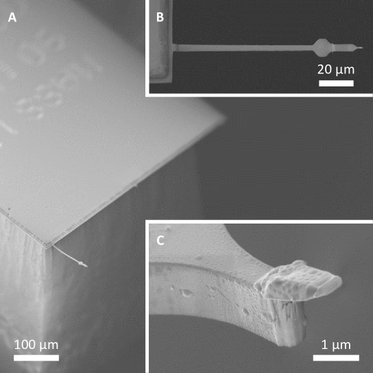
Figure 1: SEM micrograph of the Si cantilever with a GaAs sample attached. (A) shows the cantilever protruding from a Si chip. (B) clarifies the geometry showing the paddle and mass-loaded end of the cantilever, and (C) is a detailed view of the tip of the mass-loaded cantilever with the GaAs sample attached. A layer of Pt is visible at the very tip of the GaAs particle.

II Boltzmann vs. Statistical Polarization

Conventional magnetic resonance signals originate from the mean polarization of nuclear spins in an external magnetic field – the so-called Boltzmann polarization. Although this polarization is quite small, it dominates the spin signal for large ensembles of nuclear spins. As the size of the spin ensemble decreases, the amplitude of the polarization fluctuations eventually exceeds the mean polarization. Mamin:2003 This variance, sometimes called the statistical polarization, then becomes a more useful signal for MRI than the mean polarization.

Statistical polarization arises from the incomplete cancellation of randomly oriented spins. For any given direction, the net polarization can be either positive or negative and will fluctuate on a time scale that depends on the flip rate of the spins. Several MRFM experiments have detected statistical polarizations of spin-1/2 nuclear spins Mamin:2005 ; PoggioAPL:2007 ; Degen:2007 ; Degen:2008 ; Poggio:2009 ; Oosterkamp:2010 and demonstrated their use for nanometer-scale nuclear MRI. Degen:2009 ; Mamin:2009

In order to understand the regimes in which either Boltzmann or statistical polarization is important, consider an ensemble of $N$ spins with spin quantum number $I$. The Hamiltonian of a single spin in the presence of a magnetic field $B$ along the $\hat{z}$ is $\hat{H}=-\hat{\mu}_{z}B=-\hbar\gamma B\hat{I}_{z}$ where $\hat{\mu}_{z}$ is the magnetic dipole moment operator along $\hat{z}$, $\hbar$ is Planck’s constant, $\gamma$ is the gyromagnetic ratio, and $\hat{I}_{z}$ is the nuclear spin angular momentum operator along $\hat{z}$. Statistical mechanics predicts the equilibrium distribution at a temperature $T$ to be a Boltzmann distribution. The partition function $Z=Tr\{e^{-\frac{\hat{H}}{k_{B}T}}\}$ contains all the information about the nuclear spin polarization in the system. Slichter:1996 The density matrix $\hat{\rho}=\frac{1}{Z}e^{-\frac{\hat{H}}{k_{B}T}}$ of the spin system can be used to compute the mean $M_{z}=NTr\{\hat{\mu}_{z}\hat{\rho}\}$ and the variance $\sigma_{M_{z}}^{2}=N(Tr\{\hat{\mu}_{z}^{2}\hat{\rho}\}-(Tr\{\hat{\mu}_{z}\hat{\rho}\})^{2})$ of the ensemble’s magnetization along $\hat{z}$. Even at cryogenic temperatures ($T\sim 1$ K) and high magnetic fields ($B\sim 10$ T), $\hbar\gamma B\ll k_{B}T$. Therefore, keeping terms only up to first order in $\frac{\hbar\gamma B}{k_{B}T}$, we find:

$$M_{z} = N\frac{I(I+1)}{3}\hbar\gamma\left(\frac{\hbar\gamma B}{k_{B}T}\right),$$ (1)

$$\sigma_{M_{z}}^{2} = N\frac{I(I+1)}{3}\left(\hbar\gamma\right)^{2}.$$ (2)

Since $N\hbar\gamma I$ corresponds to $100\%$ spin polarization, one can define the statistical nuclear polarization as $SNP=\frac{\sigma_{M_{z}}}{N\hbar\gamma I}=\sqrt{\frac{I+1}{3I}\frac{1}{N}}$ and the Boltzmann nuclear polarization as $BNP=\frac{M_{z}}{N\hbar\gamma I}=\frac{I+1}{3}\frac{\hbar\gamma B}{k_{B}T}$. Statistical polarization dominates the system ($SNP>BNP$) when the number of spins in an ensemble is less than the critical number,

$$N_{c}=\frac{3}{I(I+1)}\left(\frac{k_{B}\,T}{\hbar\gamma B}\right)^{2}.$$ (3)

Equivalently, for a material with a nuclear spin density $na$, where $n$ is the number density of the nuclear element and $a$ is the natural abundance of the isotope of interest, one can define a critical volume $V_{c}=\frac{N_{c}}{na}$. For volumes smaller than $V_{c}$, magnetic resonance experiments should be designed to detect $SNP$ rather than $BNP$.

III MRFM Technique and Apparatus

We measure the presence of a particular nuclear isotope using an MRFM protocol which cyclically inverts statistical spin polarization. Mamin:2009 In a magnetic field $\mathbf{B_{\text{total}}}$, the frequency of a transverse RF magnetic field $\mathbf{B}_{1}$ is swept through the nuclear resonance condition, $f_{\text{RF}}=\frac{\gamma}{2\pi}B_{\text{total}}$. If done adiabatically, this sweep induces the nuclear spins to invert – a process known as adiabatic rapid passage. In the strong spatial magnetic field gradient near a magnetic tip, these inversions produce a time-dependent force. This force is in turn detected as the displacement of an ultrasensitive cantilever.

Our MRFM experiment is carried out in a sample-on-cantilever configuration in which the sample is affixed to the end of a single-crystal Si cantilever Chui:2003 as shown in Fig. 1. We arrange the cantilever in a “pendulum” geometry such that the sample is positioned above a FeCo magnetic tip, depicted in Fig. 2. The magnetic tip, which is mounted on a separate chip, is patterned on top of an Au microwire, which acts as an RF magnetic field source and is shown in Fig. 3. PoggioAPL:2007

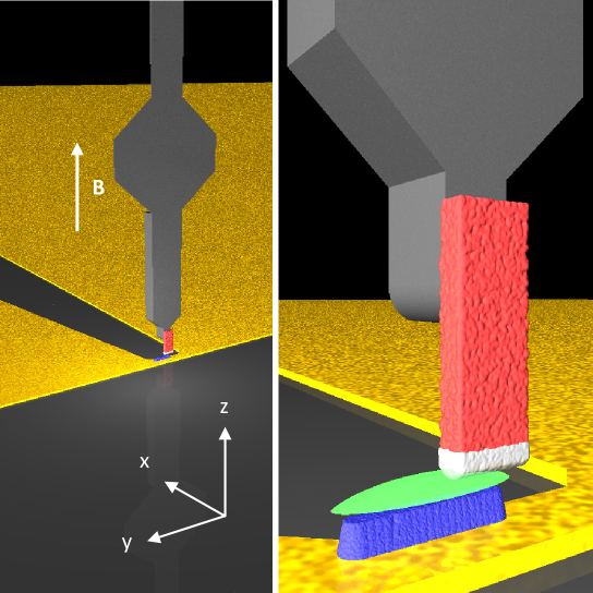
Figure 2: Representation of the MRFM apparatus at the bottom of the cryostat. The microwire is shown in yellow, the FeCo tip in blue, and the GaAs sample in red, with a Pt layer on its end in white. The green region above the FeCo tip depicts the resonant slice during measurement. $\mathbf{B}$, the cantilever shaft, and the magnetization of the FeCo tip are aligned along $\hat{z}$. Near the FeCo tip, current flows in the wire along $\hat{y}$, while the lever displacement and $\mathbf{B}_{1}$ at the position of the sample are directed along $\hat{x}$.

The cantilever measures $120\ \mathrm{\SIUnitSymbolMicro}\mathrm{m}\times 4\ \mathrm{\SIUnitSymbolMicro}\mathrm{m}\times 0.1\ \mathrm{\SIUnitSymbolMicro}\mathrm{m}$ and – loaded with the GaAs sample – has a mechanical resonance frequency $f_{c}=\omega_{c}/(2\pi)=3.7\ \mathrm{k}\mathrm{Hz}$ and an intrinsic quality factor $Q=4.0\times 10^{4}$ at $T$ = 1 K. By measuring the cantilever’s thermal motion, we determine its effective spring constant to be $k=120\ \mathrm{\SIUnitSymbolMicro}\mathrm{N}/\mathrm{m}$. The MRFM apparatus is isolated from vibrational noise and is mounted in a vacuum chamber with a pressure below $10^{-6}\ \mathrm{m}\bbar$ at the bottom of a ³He cryostat. The motion of the lever is detected using 100 nW of 1550 nm laser light focused onto a 12 $\mathrm{\SIUnitSymbolMicro}\mathrm{m}$-wide paddle and reflected back into an optical fiber interferometer. The microwire used to produce the transverse RF magnetic field is 2.5 $\mathrm{\SIUnitSymbolMicro}\mathrm{m}$-long, 1 $\mathrm{\SIUnitSymbolMicro}\mathrm{m}$-wide, and 0.2 $\mathrm{\SIUnitSymbolMicro}\mathrm{m}$-thick. The FeCo tip is shaped like a bar, sits on top of the microwire, and produces a spatially dependent field $\mathbf{B}_{\text{tip}}(\vec{r})$. It has a top width of 270 $\mathrm{n}\mathrm{m}$, a bottom width of 510 $\mathrm{n}\mathrm{m}$, a length of 1.2 $\mathrm{\SIUnitSymbolMicro}\mathrm{m}$, and a height of $265\ \mathrm{n}\mathrm{m}$ as shown in Fig. 3. To make sure that the FeCo tip is fully magnetized along the $\hat{z}$, an external magnetic field $\mathbf{B}=B\hat{z}$ is applied with $B=2.65$ T. During measurements, the distance between the FeCo tip and the closest point on the sample is typically 100 $\mathrm{n}\mathrm{m}$ such that the static magnetic field gradient $\frac{\partial B_{\text{total}}}{\partial x}$ relevant to MRFM is on the order of $5\times 10^{5}$ T/m, where $\mathbf{B}_{\text{total}}=\mathbf{B}+\mathbf{B}_{\text{tip}}$ and $\hat{x}$ is the direction of cantilever oscillation. The maximum $\left|\mathbf{B}_{\text{tip}}\right|$ for this spacing is about $0.1\ \mathrm{T}$. Smaller spacings can result is larger $\frac{\partial B_{\text{total}}}{\partial x}$ and $\left|\mathbf{B}_{\text{tip}}\right|$, although they also result in larger measurement noise. Interactions between the magnetic tip and the sample at such small gaps, known as non-contact friction, lead to mechanical dissipation in the cantilever. Stipe:2001 ; Kuehn:2006 In our experiments, these effects reduce the quality factor $Q$ of the cantilever to $1.0\times 10^{4}$. In addition, we damp $Q$ down to $\sim 400$ using active electronic feedback. Garbini:1996 Given the narrow natural bandwidth of our high-$Q$ cantilever, damping serves to increase the bandwidth of our force detection with out sacrificing signal-to-noise ratio (SNR). damping

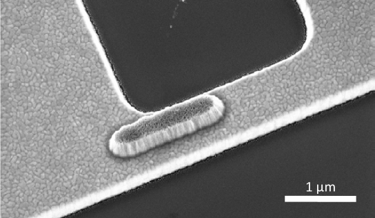
Figure 3: SEM micrograph of the Au microwire with integrated FeCo tip. The structure is patterned on a Si chip.

If the rate of the RF frequency sweeps used to invert the nuclear spins is slow enough and the amplitude of $B_{1}$ large enough, the initial population distribution among the nuclear spin energy levels is completely inverted. As a result, the net magnetization is made to flip along the $\hat{z}$. For spin-1/2 nuclei, the criterion for adiabatic inversion is given by $\alpha=2\pi\gamma^{2}B_{1}^{2}/(\omega_{c}\Omega_{\text{RF}})\gg 1$, where $\Omega_{\text{RF}}/(2\pi)$ is the amplitude of the frequency modulation around the center frequency $f_{\text{RF}}$ of the transverse RF field $B_{1}$. Slichter:1996 The criterion for quadrupolar nuclei, in general, is more complex. VanVeenendaal:1998 However, a complete inversion of the initial population distribution over the quadrupolar energy levels can be achieved in the limit of both $\alpha\gg 1$ and $\beta=\gamma B_{1}/\Omega_{\text{Q}}\gg 1$, where $\Omega_{\text{Q}}/(2\pi)$ is the quadrupolar frequency. The frequency sweeps used here are designed to meet these conditions and follow the form used in Poggio et al. PoggioAPL:2007 Therefore, by sweeping through $f_{\text{RF}}$ at a frequency $2f_{c}$, we are able to modulate the spin polarization at $f_{c}$. The resulting spin inversions produce a force that drives the cantilever at its resonance frequency. An ensemble of spins at position $\vec{r}$ with a statistical variance in its $z$-magnetization $\sigma_{M_{z}}^{2}$ produces a force on the cantilever with variance,

$$\sigma_{F}^{2}=\left(\frac{\partial B_{\text{total}}}{\partial x}(\vec{r})\right)^{2}\sigma_{M_{z}}^{2}.$$ (4)

Using our knowledge of the spring constant $k$, we determine $\sigma_{F}^{2}$ by measuring the variance of the cantilever’s oscillations on resonance. The correlation time $\tau_{m}$ of $\sigma_{F}^{2}$ is limited by the relaxation rate of the spins in the rotating frame.

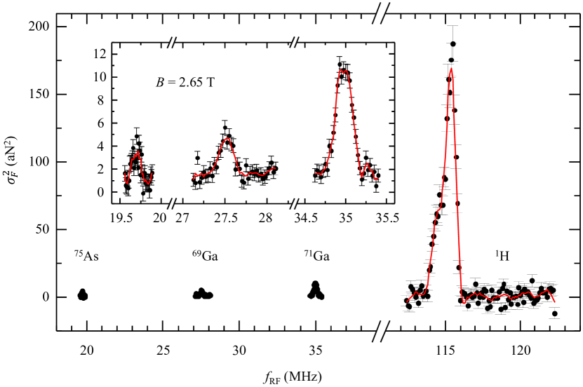
Figure 4: MRFM signal from the statistical polarization of ¹H, ⁶⁹Ga, ⁷¹Ga, and ⁷⁵As. Black dots show the resonant force variance $\sigma_{F}^{2}$ as a function of the center frequency $f_{\text{RF}}$. Solid red lines represent adjacent-averaging of the data as a guide to the eye. Inset is a zoomed-in view of the spin-3/2 nuclear resonances: ⁶⁹Ga, ⁷¹Ga, and ⁷⁵As. Error bars represent the standard error of $\sigma_{F}^{2}$ calculated as in Degen et al. Degen:2007 Data points represent 1400 s of averaging for ⁷⁵As, 600 s for ⁶⁹Ga, 600 s for ⁷¹Ga, and 300 s for ¹H.

IV Receptivity in MRFM of Statistically Polarized Ensembles

Due to differences in magnetic moment and statistical polarization, two ensembles containing the same number of nuclei but each of a different isotope, produce different magnetization variances. This difference is contained within the concept of receptivity. Receptivity is a value defined for the purpose of comparing the expected NMR signal magnitudes for equal numbers of different nuclear isotopes. For MRFM of statistically polarized ensembles, we define a receptivity, $R_{\text{N,MRFM}}\propto\gamma^{2}I(I+1)$, where $R_{\text{N,MRFM}}$ is normalized to 1 for ¹H. The factor $\gamma^{2}I(I+1)$ is proportional to the magnetization variance expected from an ensemble of spins as defined in (2). From (4) the variance, multiplied by the square of the magnetic field gradient, results in the resonant force variance measured in MRFM.

On the other hand, conventional NMR collects an inductive signal due to a Boltzmann polarization. In this case, receptivity can be defined as $R_{\text{N,conv}}\propto\gamma^{3}I(I+1)$, where $R_{\text{N,conv}}$ is similarly normalized to 1 for ¹H. Here the factor $\gamma^{2}I(I+1)$ is proportional to the Boltzmann polarization as defined in equation (1). The remaining factor of $\gamma$ results from the fact that conventional NMR measures the inductive response of a pick-up coil to magnetization precessing at a frequency proportional to $\gamma$. Callaghan:1991

As can be noted in Table 1, MRFM receptivity scales more favorably than conventional receptivity for low-$\gamma$ nuclei such as those found in GaAs. In real experiments, comparisons are often made between signals from two different isotopes contained in the same volume. In the comparison of volumes rather than number of nuclei, one must also take into account the number density $n$ of each element in the material and its natural isotopic abundance $a$. Volume receptivity therefore also includes the factors of $n$ and $a$: $R_{\text{V,MRFM}}\propto naR_{\text{N,MRFM}}$ and $R_{\text{V,conv}}\propto naR_{\text{N,conv}}$.

	1H	69Ga	71Ga	75As
	(hydrocarbon layer)	(GaAs)	(GaAs)	(GaAs)
$I$	1/2	3/2	3/2	3/2
$\frac{\gamma}{2\pi}$ (MHz/T)	42.57	10.3	13.0	7.3
$a$	1.000	0.601	0.399	1.000
$n\ (\mathrm{m}^{-3})$	$7\times 10^{28}$	$2.2\times 10^{28}$	$2.2\times 10^{28}$	$2.2\times 10^{28}$
$N_{c}$ ($B=2.65$ T, $T=1$ K)	$1.4\times 10^{5}$	$4.7\times 10^{5}$	$2.9\times 10^{5}$	$9.3\times 10^{5}$
$V_{c}$ ($B=2.65$ T, $T=1$ K)	$(12\ \mathrm{n}\mathrm{m})^{3}$	$(33\ \mathrm{n}\mathrm{m})^{3}$	$(32\ \mathrm{n}\mathrm{m})^{3}$	$(35\ \mathrm{n}\mathrm{m})^{3}$
$R_{\text{N,MRFM}}$	1	0.293	0.466	0.147
$R_{\text{N,conv}}$	1	0.071	0.142	0.025
$R_{\text{V,MRFM}}$	1	0.056	0.058	0.046
$R_{\text{V,conv}}$	1	0.013	0.018	0.008

Table 1: Properties relevant for a statistically polarized MRFM measurement.

V MRFM Measurements

Here we study a sub-micron sized particle cut from the surface of a GaAs wafer. The GaAs sample is affixed to the cantilever tip using a focused ion beam (FIB) technique. First, a thin layer of Pt is deposited over a small area of a GaAs wafer to protect the sample from potential ion damage. Then, a lamella measuring $3\ \mathrm{\SIUnitSymbolMicro}\mathrm{m}\times 2\ \mathrm{\SIUnitSymbolMicro}\mathrm{m}\times 0.3\ \mathrm{\SIUnitSymbolMicro}\mathrm{m}$ is cut out from this area of the wafer. Next, the lamella is welded with Pt to a nearby micro-manipulator and transferred to the tip of an ultrasensitive Si cantilever. Finally, the particle is Pt-welded to the cantilever tip and cut to its final dimensions: $2.4\ \mathrm{\SIUnitSymbolMicro}\mathrm{m}\times 0.8\ \mathrm{\SIUnitSymbolMicro}\mathrm{m}\times 0.3\ \mathrm{\SIUnitSymbolMicro}\mathrm{m}$ = $0.6\ \mathrm{\SIUnitSymbolMicro}\mathrm{m}^{3}$ (Fig. 1). The side of the sample which formerly was part of the wafer surface is oriented such that it faces away from the cantilever. A roughly 200 nm-thick layer of the original Pt protection layer remains on this surface of the particle. supplementary Throughout this process, only the mass-loaded end of the cantilever is exposed to either the ion or electron beams. Special care is taken never to expose the cantilever shaft to in order to avoid structural damage or deposition of material on its surface. Even short exposure can lead to the permanent bending of the cantilever and a reduction of its mechanical $Q$.

MRFM signal measured from this GaAs particle at $B=2.65$ T and temperature $T=1$ K is plotted as a function of the RF center frequency in Fig. 4. Resonances from all three isotopes (⁶⁹Ga, ⁷¹Ga, and ⁷⁵As) in GaAs are visible. In addition, a strong ¹H resonance appears in the spectrum due to the thin layer of adsorbed hydrocarbons and water that coats surfaces which have been exposed to ordinary laboratory air. Degen:2009 ; Mamin:2009 Each resonance is measured with the GaAs particle positioned at slightly different $x$ and $y$ positions in the vicinity of the FeCo tip. In each case, however, the spacing along $\hat{z}$ between the end of the particle and the top of the FeCo tip is $100\ \mathrm{n}\mathrm{m}$. Similar magnitudes of $B_{1}$ are used in each case, which we quantify in the discussion of Fig. 5. The frequency modulation amplitude $\Omega_{\text{RF}}/(2\pi)$ is 400 kHz for ¹H, 100 kHz for ⁶⁹Ga and ⁷¹Ga, and 50 kHz for ⁷⁵As. Each data point represents 300 s of averaging for ¹H, 600 s for ⁶⁹Ga and ⁷¹Ga, and 1400 s for ⁷⁵As. While the SNR for some peaks is small – ⁷⁵As and ⁶⁹Ga in particular – each peak is confirmed by at least one other experiment performed at a different magnetic field $B$. The appropriate shift in carrier frequency is observed in each case.

The rotating-frame spin correlation time $\tau_{m}$ observed for ¹H is on the order of 100 ms, which is consistent with spin correlation times measured in similar experiments on surface hydrocarbon layers. Degen:2009 ; Mamin:2009 For the quadrupolar isotopes in GaAs, we measure $\tau_{m}$ to be around 500 ms. Thurber et al. report $\tau_{m}$ on the order of several seconds in MRFM measurements of Boltzmann polarized quadrupolar spins in a GaAs wafer. Thurber:2003 Given that the adiabaticity parameter $\alpha$ is similar to that used in our experiments, the difference in $\tau_{m}$ is likely due to the large difference in magnetic field gradient in the two cases. Gradients in our experiments exceed $10^{5}\ \mathrm{T}/\mathrm{m}$ while gradients used by Thurber et al. are 100 times smaller. High magnetic field gradients on this order have been shown to limit $\tau_{m}$ in similar MRFM experiments. Degen:2008 In particular, mechanical noise originating from the thermal motion of the cantilever couples through strong magnetic field gradients to produce nuclear spin relaxation in the statistically polarized ensemble.

The central frequency, amplitude and, width of the resonance peaks depend on the various experimental parameters including $\gamma$, $B$, the spatial dependence of $B_{\text{tip}}$, the shape of the sample, its position relative to the FeCo tip, and the form of the adiabatic sweep waveform. Roughly, however, one can say that the low-frequency onset of each resonance should occur at $\frac{\gamma}{2\pi}B$. Note that the peak magnitudes in Fig. 4 do not scale with $R_{\text{V,MRFM}}$ since both the volume of the material detected and the magnetic field gradient in that volume are different for each measured peak. The striking difference in signal amplitude between the hydrocarbon layer and the quadrupolar nuclei in the GaAs particle is mostly due to the smaller gradients present inside the GaAs particle compared to those present at the hydrocarbon layer. Due to the $200\ \mathrm{n}\mathrm{m}$ Pt layer covering the tip of the GaAs particle, the ¹H containing layer is $200\ \mathrm{n}\mathrm{m}$ closer to the FeCo tip than any of the isotopes in GaAs. As a result, for the same sample tip-sample spacing, the ¹H nuclei experience about ten times higher $\frac{\partial B_{\text{total}}}{\partial x}$ than the quadrupolar isotopes – resulting in force variances 100 times larger from the same magnetization. We discuss the effect of each parameter on the resonances in more detail in Section VII.

VI Nutation Measurements

Using the method described in Poggio et al., PoggioAPL:2007 we also measure the rotating-frame amplitude of $B_{1}$. Pulses of variable length are inserted in the adiabatic sweep waveform every 500 cantilever cycles ($135\ \mathrm{m}\mathrm{s}$). The measured force variance in spin nutation experiments of ⁷¹Ga is plotted in Fig. 5 for a spacing along $\hat{z}$ between sample and FeCo tip of $100\ \mathrm{n}\mathrm{m}$. The amplitude of the rotating RF magnetic field is inferred by fitting the data to a decaying sinusoid. The frequency of the sinusoid corresponds to the Rabi frequency $\gamma B_{1}$ of the isotope in question and the decay rate is related to the spatial inhomogeneity of $B_{\text{tip}}$ within the detection volume. The measured Rabi frequency of 208 kHz for ⁷¹Ga corresponds to $B_{1}=16\ \mathrm{m}\mathrm{T}$. This measurement represents the rotating-frame amplitude $B_{1}$ in the region of the GaAs particle closest to the FeCo tip, where the gradients and the resulting contribution to the MRFM signal are largest. Similar nutation measurements done using the ¹H containing layer, which is $200\ \mathrm{n}\mathrm{m}$ closer to the FeCo tip, result in $B_{1}=17\ \mathrm{m}\mathrm{T}$. This larger measured value results from the small increase in $B_{1}$ experienced as one approaches the RF microwire source.

We calculate the Rabi frequencies at $B_{1}=16\ \mathrm{m}\mathrm{T}$ for the remaining isotopes to be 680 kHz for ¹H, 165 kHz for ⁶⁹Ga, and 117 kHz for ⁷⁵As. All isotopes satisfy the adiabaticity condition $\alpha\gg 1$. Due to cubic symmetry, no quadrupolar splitting should be present in crystalline GaAs. A small amount of strain due to the mounting process can result in a non-zero quadrupolar frequency $\Omega_{Q}$, though this splitting is likely to be on the order of 10 kHz for all isotopes. Guerrier:1997 ; Poggio:2005 In addition, for nuclear sites near the surface of the particle where symmetry is broken, electric field gradients can result in large quadrupolar splittings. Nevertheless, the large majority of the nuclear spins detected in our experiments satisfy $\beta\gg 1$. These two conditions should allow our frequency sweep waveforms to adiabatically invert all four nuclear species.

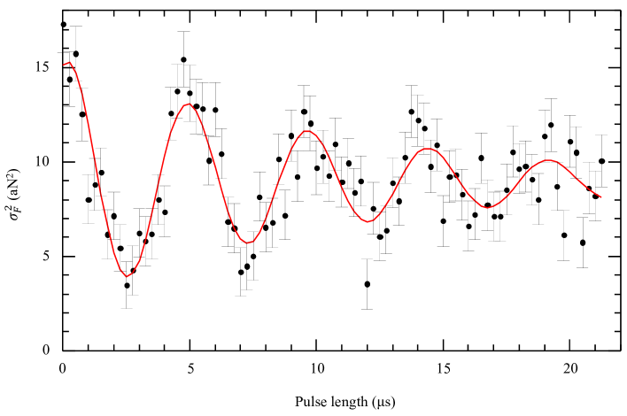
Figure 5: Nutation measurement for ⁷¹Ga at $T=1$ K. $\sigma_{F}^{2}$ from ⁷¹Ga spins is measured as a function of pulse length. A rotating-frame RF magnetic field amplitude $B_{1}$ of 16 mT is obtained from a decaying sinusoidal fit (shown in red) to the Rabi oscillations. Error bars represent the standard error of $\sigma_{F}^{2}$ calculated as in Degen et al. Degen:2007

VII Model and Estimates

Modeling the magnitude and shape of the resonance peaks shown in Fig. 4, requires both knowledge of the spatial dependence of $B_{\text{total}}(\vec{r})$ and knowledge of the shape and position of the sample. Since $B_{\text{total}}(\vec{r})$ is strongly inhomogeneous, there is a specific region in space at which the magnetic resonance condition is met for each $f_{\text{RF}}$. Only spins near these positions are adiabatically inverted and therefore included in the MRFM detection volume. This so-called “resonant slice” is a shell-like region in space above the magnetic tip whose thickness is determined by the magnetic field gradient and the modulation amplitude $\Omega_{\text{RF}}/(2\pi)$ of the frequency sweeps. We can model this region more exactly using an effective field model for adiabatic rapid passage in the manner of Section 4 of the supporting information in Degen et al. Degen:2009 This model shows that the spatial extent of the resonant slice can be described using a simple function:

$$\eta(\vec{r})= \left(1-\frac{\gamma B_{\text{total}}(\vec{r})-2\pi f_{\text{RF}}}{\Omega_{\text{RF}}}\right) \text{ for }\left(\gamma B_{\text{total}}(\vec{r})-2\pi f_{\text{RF}}\right)<\Omega_{\text{RF}}$$

$$\eta(\vec{r})= 0 \text{ for }\left(\gamma B_{\text{total}}(\vec{r})-2\pi f_{\text{RF}}\right)\geq\Omega_{\text{RF}}.$$ (5)

$\eta(\vec{r})$ is normalized to 1 for a nuclear spin positioned exactly in the middle of the resonant slice ($\gamma B_{\text{total}}(\vec{r})=2\pi f_{\text{RF}}$), signifying that this spin is fully flipped by the adiabatic passage waveform and contributes its full force to the MRFM signal. A slightly off-resonant spin with $1>\eta(\vec{r})>0$ is partially flipped and contributes a fraction of its full force to the MRFM signal. Spins outside the resonant slice with $\eta(\vec{r})=0$ contribute no signal.

In order to calculate the $\sigma_{F}^{2}$, we must therefore determine the intersection of the resonant slice with sample for each $f_{\text{RF}}$. In addition, since the gradient varies throughout the resonant slice, equal numbers of nuclei at different positions in the slice contribute different forces to the final signal. Using (2), (4), and (5) we can then integrate over the volume of the sample to find the total MRFM force variance:

$$\sigma_{F}^{2}=\int_{S}A\eta(\vec{r})\left(\frac{\partial B_{\text{total}}(\vec{r})}{\partial x}\right)^{2}na\frac{I(I+1)}{3}(\hbar\gamma)^{2}dV,$$ (6)

where $S$ is the sample volume and $A$ is a constant – usually close to 1 – which depends on the correlation time of the statistical spin polarization and the measurement detection bandwidth.

We determine $B_{\text{total}}(\vec{r})$ using a method employed in other recent MRFM experiments. Degen:2009 ; Xue:2011 First, we measure $B_{\text{total}}$ at several different positions above the FeCo tip. The maximum value of $f_{\text{RF}}$ for which a ¹H signal is obtained corresponds to the frequency where the resonant slice barely intersects hydrocarbon surface layer closest to the FeCo tip. At this frequency $f_{\text{RF,max}}$, $B_{\text{total}}(\vec{r}_{0})=\frac{2\pi}{\gamma}f_{\text{RF,max}}$ where $\vec{r}_{0}$ is the position of the hydrocarbon layer closest to the FeCo tip. Several such measurements of $B_{\text{total}}$ at different $\vec{r}_{0}$ are then used to calibrate a magnetostatic model of the FeCo tip. We infer the shape of the FeCo tip from SEM images and we assume a magnetization of $10^{6}$ A/m as in previous works. Degen:2009 ; Xue:2011 The geometrical parameters are fine-tuned in order to produce a field profile $B_{\text{tip}}(\vec{r})$ which agrees with the measured values of $B_{\text{total}}(\vec{r}_{0})=\left|\mathbf{B}+\mathbf{B}_{\text{tip}}(\vec{r}_{0})\right|$ for our known applied field $\mathbf{B}$. Our approximate model then gives us the ability to calculate both $B_{\text{total}}(\vec{r})$ and $\frac{\partial B_{\text{total}}}{\partial x}(\vec{r})$ at any position $\vec{r}$.

Given our approximate knowledge of the shape of the sample from SEM images such as Fig. 1, we can only estimate the sample volume $S$. The GaAs particle is modeled as a 2.4 $\mu$m $\times$ 0.6 $\mu$m $\times$ 0.1 $\mu$m rectangular solid with a 200-nm-thick layer of Pt on the end-face. The hydrocarbon layer is modeled as a thin film on the surface of this solid. The dimensions of this sample are meant to match the cross-sectional size of the particle closest to the FeCo tip since this part of the sample contributes nearly all of the observed $\sigma_{F}^{2}$. The back part of the sample, with larger cross-sectional area, contributes a vanishingly small $\sigma_{F}^{2}$ due to the rapid decrease in $\frac{\partial B_{\text{total}}}{\partial x}$ as a function of distance from the FeCo tip.

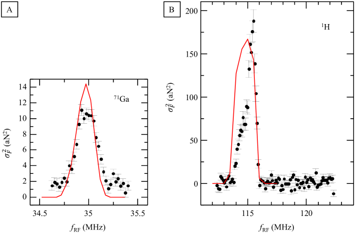
Figure 6: MRFM signal of the statistical polarization of (A) ⁷¹Ga and (B) ¹H from Fig. 4 along with the corresponding calculated signal from the our MRFM model. The sample position used in the model was matched to the experimentally set position within an error of $50\ \mathrm{n}\mathrm{m}$, likely due to experimental position drift during these long time scans. The position was fine-tuned within this error range to best match the measured signal.

We then use our models for $\mathbf{B}_{\text{total}}(\vec{r})$ and $S$ together in a numerical integration of (6) to calculate the dependence of $\sigma_{F}^{2}$ on $f_{\text{RF}}$. As shown in Fig. 6, the model reproduces the experimental data despite the approximate knowledge of the sample shape. Detailed structure within the peaks, however, is impossible to reproduce as it is often due to the nanometer-scale morphology not included in our idealized geometries. In fact, we can reproduce such large variations in the resonance peak shape by altering the details of the sample geometry used in our calculation. Prominent structure is particularly evident in resonances measured with small tip-sample spacings, where the magnetic field gradients are largest and small volumes of spins can contribute large force variances.

A thickness of 2 nm is chosen for the hydrocarbon layer in our model in order to produce a resonant $\sigma_{F}^{2}$ approximating our measurements. This thickness is consistent with previous measurements of such layers which estimated a thickness of approximately 1 nm. Degen:2009 ; Mamin:2009 The small discrepancy could be due to differences in the surface properties of our sample including roughness and affinity to adsorption of hydrocarbons compared to previous samples.

Despite the approximate nature of our model for $\sigma_{F}^{2}$, we can use it to make an order of magnitude estimate of the detection volume in our experiments. Using the parameters of each measurement, we can estimate the detection volume $V_{d}$ as the sample volume intersecting the resonant slice, i.e. the volume in which $\left(\gamma B_{\text{total}}(\vec{r})-2\pi f_{\text{RF}}\right)<\Omega_{\text{RF}}$. The number of spins contained therein is then $N_{d}=naV_{d}$. In the case of the peak $\sigma_{F}^{2}$ from the hydrocarbon layer at $f_{\text{RF}}=115.5$ MHz in Fig. 6, we calculate a $V_{d}=(40\text{ nm})^{3}$ and $N_{d}=6\times 10^{6}$. For this spin ensemble the ratio of SNP to BNP is $0.20$. Furthermore, we can estimate the sensitivity of this measurement since we know that SNR of our measurement increases with the square root of the averaging time. We calculated the SNR at each $f_{\text{RF}}$ by dividing the measured $\sigma_{F}^{2}$ by the standard error of this measurement calculated as in Degen et al. Degen:2007 This error takes into account both the noise due to fluctuations in the cantilever motion, i.e. thermal noise and non-contact friction, and the noise due to the statistically polarized spin ensemble itself. Given the SNR of 14.4 achieved after 300 s of averaging, we estimate a measurement sensitivity equivalent to $7\times 10^{6}$ ¹H spins$/\sqrt{\text{Hz}}$. In general, the sensitivity of these measurements is limited by the mechanical fluctuations of the cantilever due to thermal noise and non-contact friction.

We can make similar calculations for the quadrupolar nuclei. The peak values of $\sigma_{F}^{2}$ shown in Fig. 4, however, do not represent the maximum attainable signal for each isotope. Due to the long averaging times required for these isotopes, position scans used to optimize the signal amplitude were not performed before these measurements. Approximate measurement positions were estimated based on the ¹H experiments resulting in smaller than optimal $\sigma_{F}^{2}$. For ⁷¹Ga, however, an $x$ and $y$ position scan was performed in order to find the optimal $\sigma_{F}^{2}=25$ aN² at $f_{\text{RF}}=34.95$ MHz. From this scan it was found that changes in position less of only 50 nm resulted in signal loss of over a factor of 2, emphasizing the importance of optimal alignment. This signal is in reasonable agreement with the maximum signal $\sigma_{F}^{2}=20$ aN² calculated for the same parameters in our model. Using our model we can calculate $V_{d}=(260\text{ nm})^{3}$ and $N_{d}=2\times 10^{8}$ for the ⁷¹Ga signal plotted in Figs. 4 and 6, which is slightly shifted from the optimal position. In this case, we find $\text{SNP}/\text{BNP}=0.14$. The corresponding sensitivity is estimated from the SNR of 15.4 after 600 s of averaging to be $2\times 10^{8}$ ⁷¹Ga spins$/\sqrt{\text{Hz}}$. Similar calculations are not carried out for ⁶⁹Ga and ⁷⁵As, though sensitivity for these isotopes should be of the same order after a scaling factor equivalent to appropriate MRFM receptivity.

	1H	71Ga
	(hydrocarbon layer)	(GaAs)
Sample-tip distance $(\mathrm{n}\mathrm{m})$	100	300
Maximal $\frac{\partial B_{\text{total}}}{\partial x}$ at sample $(\mathrm{T}/\mathrm{m})$	$5\times 10^{5}$	$8\times 10^{4}$
Maximal $\left|\mathbf{B}_{\text{tip}}\right|$ at sample $(\mathrm{T})$	$0.10$	$0.03$
$f_{\text{RF}}\ (\mathrm{M}\mathrm{Hz})$	$115.5$	$34.95$
$\Omega_{\text{RF}}/(2\pi)\ (\mathrm{k}\mathrm{Hz})$	$400$	$100$
$N_{d}$	$6\times 10^{6}$	$2\times 10^{8}$
$V_{d}$	$(40\ \mathrm{n}\mathrm{m})^{3}$	$(260\ \mathrm{n}\mathrm{m})^{3}$
$\text{SNP}/\text{BNP}$	$0.29$	$0.14$
Averaging time (s)	$300$	$600$
Sensitivity $(\text{spins}/\sqrt{\text{Hz}})$	$7\times 10^{6}$	$3\times 10^{8}$

Table 2: Detection and sensitivity estimates for the ¹H and ⁷¹Ga resonances plotted in Fig. 4 at $B=2.65\mathrm{T}$ and $T=1\mathrm{K}$.

As discussed in Section V, the large difference in the sensitivity between ¹H and the quadrupolar nuclei is mostly due to the $200\ \mathrm{n}\mathrm{m}$ Pt layer which forces the Ga and As moments into a region of far smaller magnetic field gradient than at the hydrocarbon layer. Future experiments should be designed such that this Pt layer, which is an artifact of the FIB mounting process, is not present. Without this intermediate layer, far better sensitivities should be achieved for the quadrupolar nuclei. Table 3 shows predicted sensitivities for ⁶⁹Ga, ⁷¹Ga, and ⁷⁵Ga for a $100\ \mathrm{n}\mathrm{m}$ spacing between the sample and the FeCo tip – without any intermediate layer. All other parameters are identical to those of the actual experiments. These extrapolations are based on positioning the Ga and As in the same position as the ¹H nuclei in our experiment. We make the assumption that the noise would be the same as that measured in the ¹H experiment.

	69Ga	71Ga	75As
	(GaAs)	(GaAs)	(GaAs)
Sample-tip distance $(\mathrm{n}\mathrm{m})$	100	100	100
Maximal $\frac{\partial B_{\text{total}}}{\partial x}$ at sample $(\mathrm{T}/\mathrm{m})$	$5\times 10^{5}$	$5\times 10^{5}$	$5\times 10^{5}$
Maximal $\left|\mathbf{B}_{\text{tip}}\right|$ at sample $(\mathrm{T})$	$0.10$	$0.10$	$0.10$
$f_{\text{RF}}\ (\mathrm{M}\mathrm{Hz})$	$27.9$	$35.1$	$19.8$
$\Omega_{\text{RF}}/(2\pi)\ (\mathrm{k}\mathrm{Hz})$	$100$	$100$	$50$
$N_{d}$	$1\times 10^{8}$	$9\times 10^{7}$	$2\times 10^{8}$
$V_{d}$	$(210\ \mathrm{n}\mathrm{m})^{3}$	$(210\ \mathrm{n}\mathrm{m})^{3}$	$(200\ \mathrm{n}\mathrm{m})^{3}$
$\text{SNP}/\text{BNP}$	$0.20$	$0.19$	$0.23$
Calculated $\sigma_{F}^{2}\ (\text{aN}^{2})$	$250$	$210$	$150$
Sensitivity $(\text{spins}/\sqrt{\text{Hz}}$)	$1\times 10^{8}$	$9\times 10^{7}$	$3\times 10^{8}$

Table 3: Extrapolated detection and sensitivity estimates for the quadrupolar nuclei based on parameters achieved for ¹H at $B=2.65\mathrm{T}$ and $T=1\mathrm{K}$ in Table 2.

VIII Conclusion

The results presented here, demonstrate our ability to detect nanometer-scale volumes of Ga and As nuclei using MRFM. Given the spin sensitivity extrapolated from our data and our model, the detection of III-V nanostructures such as nanowires or sub-surface self-assembled InAs QDs should be possible. Self-assembled InAs QDs, for example, contain $10^{5}$–$10^{7}$ nuclear spins, lie as close as $50\ \mathrm{n}\mathrm{m}$ from the wafer surface, and could be attached to a cantilever using the FIB technique demonstrated here. Further improvements to the force sensitivity – most importantly for reducing measurement times – will be required in order to realize MRI in III-V materials with better than 100 nm resolution. The potential for sub-surface, isotopically selective imaging on the nanometer-scale in III-V materials is a particularly exciting prospect since conventional methods such as SEM and TEM lack isotopic contrast.

- (1) L. Ciobanu, D. A. Seeber, and C. H. Pennington, J. Magn. Reson. 158, 178 (2002).
- (2) M. Poggio and C. L. Degen, Nanotechnology 21, 342001 (2010).
- (3) C. L. Degen, M. Poggio, H. J. Mamin, C. T. Rettner, and D. Rugar, Proc. Nat. Acad. Sci. USA 106, 1313 (2009).
- (4) R. Verhagen, A. Wittlin, C. W. Hilbers, H. van Kempen, and A. P. M. Kentgens, J. Am. Chem. Soc. 124, 1588 (2002).
- (5) K. R. Thurber, L. E. Harrell, R. Fainchtein, and D. D. Smith, Appl. Phys. Lett. 80, 1794-1796 (2002).
- (6) K. R. Thurber, L. E. Harrell, and D. D. Smith, J. Magn. Reson. 162, 336-340 (2003).
- (7) S. R. Garner, S. Kuehn, J. M. Dawlaty, N. E. Jenkins, J. A. Marohn, Appl. Phys. Lett. 84, 5091 (2004).
- (8) H. J. Mamin, R. Budakian, B. W. Chui, and D. Rugar, Phys. Rev. Lett. 91, 207604 (2003).
- (9) H. J. Mamin, R. Budakian, B. W. Chui, and D. Rugar, Phys. Rev. B 72, 024413 (2005).
- (10) M. Poggio, C. L. Degen, C. T. Rettner, H. J. Mamin, and D. Rugar, Appl. Phys. Lett. 90, 263111 (2007).
- (11) C. L. Degen, M. Poggio, H. J. Mamin and D. Rugar, Phys. Rev. Lett. 99, 250601 (2007).
- (12) C. L. Degen, M. Poggio, H. J. Mamin and D. Rugar, Phys. Rev. Lett. 100, 137601 (2008).
- (13) M. Poggio, H. J. Mamin, C. L. Degen, M. H. Sherwood, and D. Rugar, Phys. Rev. Lett. 102, 087604 (2009).
- (14) T. H. Oosterkamp, M. Poggio, C. L. Degen, H. J. Mamin, and D. Rugar, Appl. Phys. Lett. 96, 083107 (2010).
- (15) H. J. Mamin, T. H. Oosterkamp, M. Poggio, C. L. Degen, C. T. Rettner and D. Rugar, Nano Letters 9, 3020 (2009).
- (16) C. P. Slichter, Principles of Magnetic Resonance (Springer, Berlin, 1990), 3rd ed.
- (17) B. W. Chui, Y. Hishinuma, R. Budakian, H. J. Mamin, T. W. Kenny, and D. Rugar, TRANSDUCERS, 12th International Conference on Solid-State Sensors, Actuators and Microsystems 2, 1120 (2003).
- (18) B. C. Stipe, H. J. Mamin, T. D. Stowe, T. W. Kenny, and D. Rugar, Phys. Rev. Lett. 87, 096801 (2001).
- (19) S. Kuehn, R. F. Loring, and J. A. Marohn, Phys. Rev. Lett. 96, 156103 (2006).
- (20) J. L. Garbini, K. J. Bruland, W. M. Dougherty, and J. A. Sidles, J. Appl. Phys. 80, 1951 (1996); K. J. Bruland, J. L. Garbini, W. M. Dougherty, and J. A. Sidles, J. Appl. Phys. 80, 1959 (1996).
- (21) Without damping by electronic feedback, the SNR of a thermally-limited force measurement is given by the ratio of the signal force to the thermal force acting on the cantilever , where is a measurement bandwidth much smaller than the cantilever bandwidth. This ratio is preserved even in the presence of electronic damping, since the damping reduces the amplitude and broadens the spectrum of any cantilever motion. Cantilever motion caused by either or is reduced equally and therefore the SNR and the force sensitivity (the size of the force required for an SNR of 1) remain unchanged. The spectral width of the cantilever motion, however, is broadened by damping, allowing for larger and thus for the measurement of forces with faster correlation times.
- (22) E. Van Veenendaal, B. H. Meier, and A. P. M. Kentgens, Mol. Phys. 93, 195 (1998).
- (23) P. T. Callaghan, Principles of Nuclear Magnetic Resonance Microscopy (Oxford University Press, Oxford, 1991), p. 174.
- (24) See supplementary material for a description of the FIB process.
- (25) Fei Xue, P. Peddibhotla, M. Montinaro, D. P. Weber, and M. Poggio, Appl. Phys. Lett. 98, 163103 (2011).
- (26) D. J. Guerrier and R. T. Harley, Appl. Phys. Lett. 70, 1739 (1997).
- (27) M. Poggio and D. D. Awschalom, Appl. Phys. Lett. 86, 182103 (2005).