Abstract. Stability of the kink-like and soliton-like travelling wave solutions to the generalized convection-reaction-diffusion equation is studied by means of the qualitative methods and numerical simulation.

Keywords: generalized transport equation, active media, temporal non-locality, traveling wave solutions, stability of wave patterns

1 Introduction

In this work we discuss the stability of traveling wave (TW) solutions of the following family of convection-reaction-diffusion equations:

$$\tau\,u_{tt}+u_{t}+g(u)\,u_{x}=\left[\kappa(u)\,u_{x}\right]_{x}+f(u).$$ (1)

Here $\tau\geq 0,$ $f(u)$ and $g(u)$ are peace-wise continuous functions, $\kappa(u)$ is smooth and positive for $u>0$. Equations belonging to this family attracted attention of many authors. The case $\tau=0$, recognized as convection-reaction-diffusion (CRD) equation, is the subject of investigations in several monographs [1, 2, 3, 4]. It is widely used to describe transport phenomena in porous media [5], theory of combustion and detonation [6], and mathematical biology [7, 8].

Besides the various applications, the CRD equation is valuable as the simplest nonlinear model of transport phenomena having in some cases nontrivial symmetry and, thus, possessing many exact solutions and conservation laws [9, 10, 11, 12, 13, 14, 15].

General concepts leading to the family (1) with $\tau\neq 0$ can be found in papers [16, 17, 18, 19]. It can be formally introduced if one changes in the balance equation the convenient Fick’s law

$$J(t,\,x)=-\nabla\,q(t,\,x),$$

stating the thermodynamical flow-force relations, with the Cattaneo’s equation

$$\tau\frac{\partial\,J(t,\,x)}{\partial\,t}+J(t,\,x)=-\nabla\,q(t,\,x),$$

which takes into account the effects of memory.

Physically meaningful TW solutions to Eq. (1), such as periodic, kink-like and, soliton-like solutions, compactons, shock fronts, cuspons, and many other are either shown to exist or exactly constructed in papers [20, 21, 22, 23, 19, 24, 25].

The aim of this work is to analyze the stability of kink-like and soliton-like TW solutions to Eq. (1). The structure of the work is following. In section 2 a geometric insight into the family of TW solutions is made, and the linearized equations describing the evolution of small perturbations of TW solutions, taking the form of spectral problem are derived. In section 3 some important properties of the continuous spectrum are stated, and the stability of the constant asymptotic solutions is studied. In section 4 some statements concerning the discrete spectrum are formulated. In section 5 the results of numerical study of the temporal evolution of the kink-like and soliton-like TW solutions, confirming and supplementing the results of qualitative studies, are presented.

2 Geometric insight into the TW solutions, and the statement of the problem

This work is devoted to the analysis of stability the TW solutions having the form

$$u(t,\,x)=U(z),\quad z=x-s\,t,$$ (2)

where $s$ stands for the velocity of the traveling wave. To begin with, let us make the geometric interpretation of some of the TW solutions. Substituting the ansatz (2) into the source equation, we obtain the following ordinary differential equation:

$$\Delta U^{\prime\prime}(z)=\dot{\kappa}(U)\,{U^{\prime}}^{2}+\left[s-g(U)\right]\,{U^{\prime}}+f(U),$$ (3)

where $\Delta=\tau\,s^{2}-{\kappa}(U)$, both symbols $\dot{(\cdot)}$, and ${(\cdot)^{\prime}}$ stand for the derivative. This equation can be presented in the form of the dynamical system

$$\begin{array}[]{l}\Delta\,U^{\prime}(z)=\Delta\,W(z),\\ \Delta\,W^{\prime}(z)=\dot{\kappa}(U)\,W^{2}+\left[s-g(U)\right]\,W+f(U).\end{array}$$ (4)

Now let us formulate a simple statements concerning the dynamical system (4) and the properties of its solutions.

1. The stationary points of the system (4) belong to either the horizontal axis, or singular line $\Delta=0.$

2. A smooth kink-like solution is represented in the phase plane $(U,\,\,W)$ by the heteroclinic trajectory, which does not intersect the singular line $\Delta=0$ (see Fig. 1)

3. The soliton-like solution is represented by the trajectory bi-asymptotic to a saddle point which does not belong to the singular line $\Delta=0$ (see Fig. 2).

4. The trajectory bi-asymptotic to a saddle point lying in the singular line $\Delta=0$ can correspond to either compacton, or shock front (fore more detail see [25, 26]).

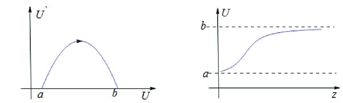
Figure 1: Left: the heteroclinic trajectory in the phase plane $(U,\,U^{\prime})$; right: the corresponding kink-like solution $U(z)$

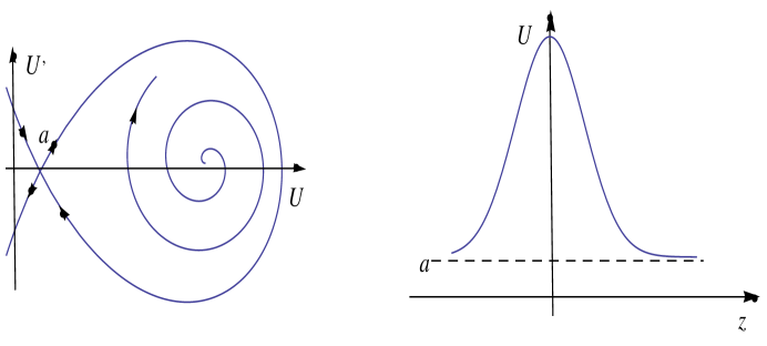
Figure 2: Left: the homoclinic trajectory in the phase plane $(U,\,U^{\prime})$; right: the corresponding soiton-like solution $U(z)$

Let us note that obtaining the analytical description to solitons, compactons, or shock fronts in case of a typical dissipative system like (4) is rather difficult. But it is much more easy to ”capture” the homoclinic trajectory through two bifurcations: the Hopf bifurcation, followed by the homoclinic bifurcation (see Fig. 3). The Hopf bifurcation can be predicted by means of the local asymptotic analysis [27, 28]. The homoclinic bifurcation is nonlocal, and therefore should be captured numerically [29, 25].

A simple analysis shows, that the equation (1) can have the homoclinic or heteroclinic TW solutions, if the corresponding dynamical system possess at least two stationary points. This, in turn, determines the form of the source term $f(u)$, which in the simplest case is as follows:

$$f(U)=(U-U_{1})\,(U-U_{0})\,\Psi(U).$$ (5)

We assume that $U_{0}\,<\,U_{1}$, and $\Psi(U)$ does not intersect the horizontal axis within the interval $(U_{0},\,U_{1}).$

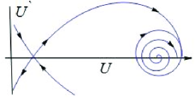
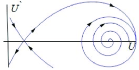
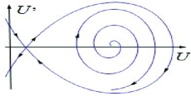
Figure 3: Birth of the bi-asymptotic trajectory. Left: periodic trajectory created as a result of the Hopf bifurcation; middle: the change of driving parameter causes the grows of the radius of periodic trajectory, which is finally destroyed as a result of the interaction with the nearby saddle point (right)

Let us now concentrate upon the problem of stability of the TW solution (2). Since we are interested in studying the stability of kink-like and soliton-like solutions, then we assume, that

$$\lim\limits_{z\to\pm\infty}\,U(z)=m_{\pm},$$ (6)

where $m_{\pm}$ are the constants coinciding with $U_{0}$ or $U_{1}$ (in the case of a kink-like solution $m_{+}\,\neq\,m_{-}$, in the case of soliton-like solution $m_{+}\,=\,m_{-}=U_{0}$). We assume in addition, that

$$\lim\limits_{z\to\pm\infty}\,U^{(k)}(z)=0$$ (7)

for any natural $k$.

To study the stability of a TW solution $U(z),$ we use the ansatz

$$u(t,\,x)=U(z)+\epsilon\,\exp{[\lambda\,t]}\,v(z),$$ (8)

where $\lambda$ is the spectral parameter, and $|\epsilon|\ll\,1.$ It is instructive to pass to new independent variables

$$\bar{t}=t,\qquad\bar{z}=x-s\,t,$$

in which the invariant solution (2) becomes stationary. In the new variables the equation (1) reads as follows:

$$\tau\,\left[\frac{\partial}{\partial\,\bar{t}}-s\frac{\partial}{\partial\,\bar{z}}\right]^{2}\,u+\left[\frac{\partial}{\partial\,\bar{t}}-s\frac{\partial}{\partial\,\bar{z}}\right]\,u+g(u)\,\frac{\partial\,u}{\partial\,\bar{z}}-\frac{\partial}{\partial\,\bar{z}}\left[\kappa(u)\,\frac{\partial\,u}{\partial\,\bar{z}}\right]=f(u)$$ (9)

(for simplicity, we omit the bars over the independent variables henceforth). Up to $O(\epsilon^{2})$, the function $v(z)$ satisfies the equation

$$L\,\left[z,\,\frac{d}{d\,z},\,\lambda\right]\,v(z)=\left\{\Delta\,\frac{d^{2}}{d\,z^{2}}+\left[g(U)-2\,\dot{U}\,\dot{\kappa}(U)-s(1+2\,\tau\,\lambda)\right]\,\frac{d}{d\,z}+\right.$$ (10)

$$\left.+\lambda(1+\tau\,\lambda)+\dot{g}(U)\dot{U}-\dot{\kappa}(U)\,\ddot{U}-\ddot{\kappa}(U)\dot{U}^{2}-\dot{f}(U)\right\}\,v(z)=0,$$

where $\Delta\,=\tau\,s^{2}-\kappa(U)$.

Definition 1. The set of all possible values of $\lambda\,\in\,\mathbb{C}$ for which the variational equation (10) has nontrivial solutions is called the spectrum of the operator $L\,\left[z,\,\frac{d}{d\,z},\,\lambda\right]$.

Definition 2. We say that the TW solution $U(z)$ is (linearly) stable, if any possible eigenvalue $\lambda$ for which the equation (10) has nonzero solution satisfies the condition $\lambda\,\in\,\mathbb{C}\cup\,{0}$.

Remark. It is easily seen, that zero eigenvalue always belongs to the spectrum of the operator $L\,\left[z,\,\frac{d}{d\,z},\,\lambda\right]$, for the following statement holds:

Lemma. If $U(z)$ is a TW solution of the equation (1), then $v_{\nu}(z)=\dot{U}(z)$ is the eigenvector of the operator $L\,\left[z,\,\frac{d}{d\,z},\,0\right]$.

Proof. Differentiating (3) w.r.t. $z$, we can rewrite the resulting equation in the form:

$$\left\{\left[\tau\,s^{2}-\kappa(U)\right]\,\frac{d^{2}}{d\,z^{2}}+\left[g(U)-2\,\dot{U}\,\dot{\kappa}(U)-s\right]\,\frac{d}{d\,z}+\right.$$

$$\left.+\dot{g}(U)\dot{U}-\dot{\kappa}(U)\,\ddot{U}-\ddot{\kappa}(U)\dot{U}^{2}-\dot{f}(U)\right\}\,v_{\nu}(z)=0,$$

where $v_{\nu}(z)$ stands for $\dot{U}(z).$ The differential operator inside the braces coincides with $L\,\left[z,\,\frac{d}{d\,z},\,\lambda\right]$, when $\lambda=0.$ $\Box$

As usually, we distinguish the continuous spectrum $\sigma_{cont}\,\subset\,\mathbb{C},$ and the discrete spectrum $\sigma_{discr}\,\subset\,\mathbb{C}.$ Being somewhat informal, we can treat $\sigma_{cont}$ as the subset responsible for the stability of the stationary solutions $m_{\pm}$, and $\sigma_{discr}$ for the stability of the solution $U(z)$ itself.

3 Stability of the asymptotic stationary solutions

Now we are going to state the conditions which guarantee that $\sigma_{cont}\,\subset\,\mathbb{C}^{-}$. For this purpose, we study the stability of the stationary solution $U_{k}=\mbox{const}$, assuming that it coincides with $m_{+}$ or $m_{-}$. We assume in addition that the eigenvectors of the operators $L\,\left[\pm\,\infty,\,\frac{d}{d\,z},\,\lambda\right]$ belong to the space of tempered distributions $\mathcal{S^{\prime}(R)}$ [30]. With this assumption, we can solve the spectral problem

$$L\,\left[\ell,\,\frac{d}{d\,z},\,\lambda\right]v(z)=0,$$ (11)

where $\ell$ stands for plus or minus infinity, by applying to this equation the Fourier transformation. Thus, assuming that $\lim\limits_{z\to\ell}U(z)=U_{k},$ we get:

$$\begin{array}[]{l}F\left\{L\,\left[\ell,\,\frac{d}{d\,z},\,\lambda\right]\,v\right\}[\xi]=\\ =L\,\left[\ell,\,-i\,\xi,\,\lambda\right]\,F[v](\xi)=\\ =\left\{-\left[\tau\,s^{2}-\kappa(U_{k})\right]\,\xi^{2}-i\,\xi\,\left[g\left(U_{k}\right)-s\,(1+2\,\lambda\,\tau)\right]+\lambda\,(1+\lambda\,\tau)-\dot{f}\left(U_{k}\right)\right\}\,F[v](\xi)=0.\end{array}$$

This equation has nonzero solution $F[v](\xi)\,\in\,\mathcal{S^{\prime}(R)}$ if

$$\lambda=\frac{-(1+2i\,s\,\tau\,\xi)\pm\sqrt{Q}}{2\,\tau},$$ (12)

where

$$Q=1-4\tau\kappa\xi^{2}+4\tau\dot{f}(U_{k})+4\,i\,\tau\xi\,g\left(U_{k}\right).$$

Since we are going to estimate the real part of $\lambda$, it is instructive to use the representation

$$\sqrt{Q}=x+i\,y,\quad\mbox{with}\quad x,\,\,y\,\in\mbox{R}.$$

Raising both sides of this equation to the second power, and eliminating $y$, we get the bi-quadratic equation

$$x^{4}-x^{2}\left[1-4\tau\kappa\xi^{2}+4\tau\dot{f}(U_{k})\right]-4\tau^{2}\xi^{2}g(U_{k})^{2}=0.$$

Its positive root takes the form

$$x=\frac{1}{\sqrt{2}}\,\left[1-4\tau\kappa\xi^{2}+4\,\tau\dot{f}(U_{k})+\sqrt{Q_{1}}\right]^{1/2},$$

where

$$Q_{1}=\left(1-4\tau\kappa\xi^{2}+4\tau\dot{f}(U_{k})\right)^{2}+16\tau^{2}\xi^{2}g^{2}(U_{k}).$$

So the biggest real part of $\lambda$, which we denote by $Re\,\lambda^{+}$, is as follows:

$$Re\,\lambda^{+}=\frac{1}{2\tau}\left\{-1+\frac{1}{\sqrt{2}}\left[1-4\tau\kappa\xi^{2}+4\,\tau\dot{f}(U_{k})+\sqrt{Q_{1}}\right]^{1/2}\right\}.$$

Let us solve the inequality $Re\,\lambda^{+}\,<\,0$ with respect to $\xi\,\in\,{\mathbb{R}}$. It is equivalent to the inequality

$$\left[1-4\tau\kappa\xi^{2}+4\,\tau\dot{f}(U_{k})+\sqrt{Q_{1}}\right]^{1/2}\,<\,\sqrt{2},$$

which, in turn, can be rewritten as

$$\sqrt{Q_{1}}\,<\,1+4\tau\kappa\xi^{2}-4\,\tau\dot{f}(U_{k}).$$

Rasing both sides of this inequality to the second power, we get, after some algebraic manipulation, the inequality

$$\xi^{2}\left[\tau g^{2}(U_{k})-\kappa(U_{k})\right]\,<\,-\dot{f}(U_{k}),$$ (13)

which should be fulfilled for any $\xi\,\in\mathbb{R}.$ So the following statement is true.

Statement1. The stationary solution $U_{k}$ is stable if

$$\tau g^{2}(U_{k})-\kappa(U_{k})\,<\,0,\quad\mbox{and}\quad\dot{f}(U_{k})<0.$$

In order to get $\sigma_{cont}$ in case $\tau=0$, we have to consider the eigenvalue problem

$$\begin{array}[]{l}L_{1}\left[\ell,\,\frac{d}{d\,z}\right]\,v(z)=\\ =\left\{\kappa(U_{k})\frac{d^{2}}{d\,z^{2}}+\left[s-g(U_{k})\right]\,\frac{d}{d\,z}+\dot{f}(U_{k})\right\}\,v(z)=\lambda\,v(z).\end{array}$$

Applying the Fourier transformation, we get

$$\lambda=i\,\xi\,\left[g(U_{k})-s\right]-\kappa(U_{k})\,\xi^{2}+\dot{f}(U_{k}),\quad\xi\,\in\,\mbox{R}.$$

So in the case $\tau=0$, we obtain the following result.

Statement 2. If for $U_{k}=\lim\limits_{z\to\,\ell}U(z)$ $\dot{f}\left[U_{k}\right]<0$, $k=0,\,1$ then $\sigma_{cont}\,\in\,\mathbb{C^{-}}$.

4 Some remarks concerning the discrete spectrum

We remind that if the function $U(z)$ is the TW solution of the equation (1), then its derivative $\dot{U}(z)$ is the eigenvector of the operator $L\left[z,\,\frac{d}{d\,z},\,0\right]$, corresponding to the eigenvalue $\lambda=0.$ This fact plays very important rule when $\tau=0$, for it is possible to address the question of stability of soliton-like and kink-like solutions by employing the classical Sturm-Liouville theory [31]. Let us shortly remind one of its conclusions.

Theorem (Sturm Oscillation Theorem). Let $\lambda_{0}>\lambda_{2}>...$ be the eigenvalues of the spectral problem

$$\left\{H\left[z,\,\frac{d}{d\,z}\right]\right\}\,u(z)=\left\{\frac{d^{2}}{d\,z^{2}}+V(z)\right\}\,u(z)=\lambda\,u(z),\qquad\lim\limits_{z\to A}u(z)=\lim\limits_{z\to B}u(z)=0,$$

where $u(z)\,\in\,L^{2}(A,\,B)$, $(A,\,B)\in\,\mathbb{R}$, is finite or infinite interval, $V(z)$ is a bounded function. Then the eigenvector $u(z,\,\lambda_{n})$ has exactly $n$ zeroes in $(A,\,B)$.

Let us consider the eigenvalue problem for the case $\tau=0$, assuming in addition that $\kappa=\mbox{const}.$ Then we can rewrite the variational equation (10) in the form

$$\left[\frac{d^{2}}{d\,z^{2}}+a(z)\frac{d}{d\,z}+b(z)\right]\,v(z)=\tilde{\lambda}\,v(z),$$ (14)

where $\tilde{\lambda}=\lambda/\kappa,$

$$a(z)=\frac{s-g(U)}{\kappa},\qquad b(z)=\frac{\dot{f}(U)-\dot{U}\,\dot{g}(U)}{\kappa}.$$

The problem (14) can be presented in the standard Sturm-Liouville form, if we use the following transformation:

$$v(z)=\exp\left[\varphi(z)\right]\,w(z),\qquad\mbox{where}\qquad\dot{\varphi}(z)=-\frac{a(z)}{2}.$$ (15)

Using (15), we obtain the eigenvalue problem

$$\left[\frac{d^{2}}{d\,z^{2}}+\Phi(z)\right]\,w(z)=\tilde{\lambda}\,w(z),$$ (16)

where

$$\Phi(z)=b(z)-\frac{a^{2}(z)}{4}-\frac{a(z)}{2}.$$

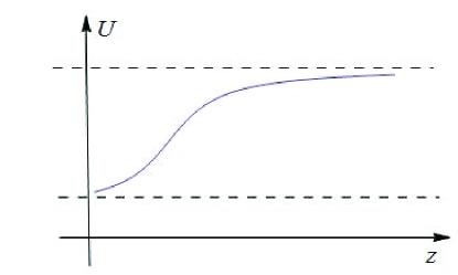
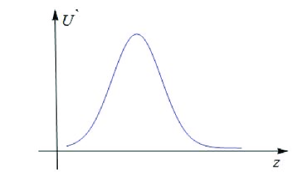
Figure 4: Graphs of the monotonic kink-like solution (left), and its derivative (right)

By $w_{\nu}(z)$ we denote the eigenvector corresponding to the eigenvalue $\tilde{\lambda}_{\nu}=0.$ And now, if $U(z)$ is the kink with the monotone profile, then $v_{\nu}(z)=\dot{U}(z)$, as well as $w_{\nu}(z)=\dot{U}(z)\,\exp\left[-\varphi(z)\right]$, is a functions, which does not intersect the real axis, see Fig 4. Then on virtue of the Sturm Oscillation Theorem, $\tilde{\lambda}_{\nu}=\tilde{\lambda}_{0}=0$, and all the remaining eigenvalues are negative.

On the other hand, if $U(z)$ is the soliton-like TW solution, then both $v_{\nu}(z)=\dot{U}(z)$, and $w_{\nu}(z)=\dot{U}(z)\,\exp\left[-\varphi(z)\right]$ intersect the horizontal axis, see Fig 5. So $\tilde{\lambda}_{\nu}=\tilde{\lambda}_{1}=0$, and there is the eigenvalue $\tilde{\lambda}_{0}\,>0$ belonging to the right half-plane of the complex plane. The latter result is rather well-known [32]. Conditions concerning the stability of kink-like solution can be formulated as follows.

Statement 3. A monotonic kink-like solution of the equation (1) with $\tau=0$ is stable, provided that $\dot{f}(U_{k})<0$ for $k=0,\,1.$

It is possible to apply the approach based on the Sturm-Liouvliie theory in the case when $\tau>0$, and $g(u)$, $\kappa(u)$ are constant functions. Under these conditions, the variational equation can be presented in the form

$$\left[\frac{d^{2}}{d\,z^{2}}+\tilde{a}(z)\frac{d}{d\,z}+\tilde{b}(z)\right]\,v(z)=\theta\,v(z),$$ (17)

where

$$\tilde{a}(z)=\frac{s\,(1+2\,\tau\,\lambda)-g}{\mu},\quad\tilde{b}(z)=\frac{\dot{f}(U)}{\mu},\quad\theta=\frac{\lambda(1+\tau\,\lambda)}{\mu},$$

$\mu=\kappa-\tau\,s^{2}$, The transformation

$$v(z)=\exp\left[\varphi(z)\,w(z)\right],\qquad\mbox{where}\qquad\dot{\varphi}(z)=\frac{g-s(1+2\,\tau\,\lambda)}{2\,\mu}$$

leads in this case to the spectral problem

$$\left[\frac{d^{2}}{d\,z^{2}}+\Psi(z)\right]\,w(z)=\chi(\lambda)\,w(z),\quad\lim\limits_{z\to a}w(z)=\lim\limits_{z\to b}w(z)=0,$$

where

$$\Psi(z)=\frac{g(2\,s-g)-s^{2}}{4\,\mu^{2}}+\frac{\dot{f}[U(z)]}{\mu},\qquad\chi(\lambda)=\frac{\lambda[\kappa-g\,s\,\tau+\kappa\,\tau\,\lambda]}{\mu^{2}}.$$

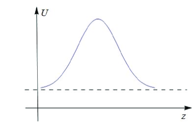
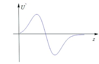
Figure 5: The graphs of one-humped soliton-like solution $U(z)$ (left), and its derivative $\dot{U}(z)$ (right)

Thus, if $U(z)$ is a monotonic kink-like solution, then $v_{0}(z)=\dot{U}(z)$ is the eigenvector corresponding to the eigenvalue $\lambda=0.$ The corresponding function $w_{0}(z)=e^{-\varphi(z)}\,v_{0}(z)$ is the eigenvector of the operator $\hat{H}=\frac{d^{2}}{d\,z^{2}}+\Psi(z)$. Since the function $w_{0}(z)$ does not intersect the horizontal axis, then, on virtue of the Sturm Oscillation Theorem, it corresponds to the eigenvalue $\chi_{0}=0$, and any other eigenvalue of this problem is negative. But $\chi(\lambda)$ is the quadratic function of $\lambda$, and therefore the source eigenvalue problem (17) can have an extra eigenvalue, corresponding to the function $\dot{U}(z).$ This extra root will be negative, if the constant $\kappa-g\,s\,\tau,$ is positive, and negative otherwise, see Fig. 6. Hence for $\tau>0$ we get an extra condition

$$\kappa-g\,s\,\tau\,>\,0,$$ (18)

assuring that $\sigma_{discr}\,\in\,C^{-}.$

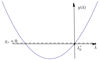
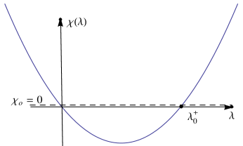
Figure 6: Graphs of the function $\chi(\lambda)$ and the eigenvalues $\lambda_{0}^{+}$ corresponding to $\dot{U}(z)$ when ${U}(z)$ is a kink-like TW solution. Left: $\kappa-g\,s\,\tau>0$; right: $\kappa-g\,s\,\tau<0$

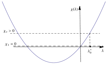
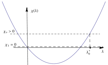
Figure 7: Graphs of the function $\chi(\lambda)$ and the eigenvalues $\lambda_{0}^{+}$ corresponding to $\dot{U}(z)$ when ${U}(z)$ is a soliton-like TW solution. Left: $\kappa-g\,s\,\tau>0$; right: $\kappa-g\,s\,\tau<0$

If, in turn, $U(z)$ is the soliton-like solution, then the eigenvector $w_{\nu}=\exp{[-\varphi(z)]}\,\dot{U}(z)$ corresponding to the eigenvalue $\chi_{\nu}=0$ intersects once the horizontal axis. Hence $\nu=1,$ and there is an extra eigenvalue $\chi_{0}>\chi_{1}=0$, to which corresponds a pair of the eigenvalues $\lambda_{0}^{\pm}$ of the source eigenvalue problem. As it is seen in Fig. 7, regardless of the sign of $\kappa-g\,s\,\tau$, there exists the positive eigenvalue $\lambda_{0}^{+}$, hence the soliton-like solution is unstable.

5 The results of numerical simulations

In the general case, i.e., when, e.g., the function $g(u)$ is not constant, estimation of $\sigma_{discr}$ is rather more delicate problem. In paper [33] such estimation is performed for the TW solution

$$u(t,\,x)=U(z)=\frac{\Psi^{\prime}(z)}{\Psi(z)},\qquad\Psi(z)=\exp{[m_{1}\,z]}+C_{2}\,\exp{[m_{2}\,z]}+C_{3}\,\exp{[m_{3}\,z]},$$ (19)

satisfying the equation

$$\tau\,u_{tt}+u_{t}+\mu\,u\,u_{x}=\kappa\,u_{x\,x}+\nu\,(u-m_{1})\,(u-m_{2})(u-m_{3}),$$ (20)

under the following restrictions on the parameters:

$$\mu=3\,\Delta,\quad\nu=-\Delta,\quad s=(m_{1}+m_{2}+m_{3})\,\Delta\equiv\,\frac{1+\sqrt{1+4\,\tau\,\kappa(\sum_{k=1}^{3}{m_{k}})^{2}}}{2\,\tau\,\sum_{k=1}^{3}{m_{k}}}$$

Unfortunately, $\sigma_{cont}$ for none of these solutions is contained in $\mathbb{C^{-}}$, as will be shown below.

Statement 4. If $C_{2}^{2}+C_{3}^{2}>0$, and $0\,\leq\,m_{1}<m_{2}<m_{3}$, then the stationary point $m_{+}=\lim\limits_{z\,\to\,+\infty}U(z)$ is unstable.

Proof. The stationary point $U_{k}=m_{+}$ is stable, if the inequality (13) is fulfilled for all $\xi\in\,\mathbb{R}$. The case $C_{3}=0$ is very easy to analyze. Indeed, under this assumption $m_{+}$ coincides with $m_{2}$, and thus

$$\dot{f}(m_{2})=\nu\,(m_{2}-m_{1})\,(m_{2}-m_{3})=-\Delta\,(m_{2}-m_{1})\,(m_{2}-m_{3})>0.$$

Hence the conditions of the statement 1 are not fulfilled.

If $C_{3}\,\neq\,0$, then $\lim\limits_{z\,\to\,+\infty}=m_{3}$, and

$$\dot{f}(m_{3})=\nu\,(m_{3}-m_{1})\,(m_{3}-m_{2})=-\Delta\,(m_{3}-m_{1})\,(m_{3}-m_{2})<0.$$

Let us address the condition

$$\tau\,g^{2}(m_{3})-\kappa\,=\,\tau\,(\mu\,m_{3})^{2}-\kappa\,=\,\tau(3\,\Delta\,m_{3})-\kappa\,<\,0.$$

This inequality is equivalent to the following one:

$$\Delta\,=\,\frac{1+\sqrt{1+4\,\tau\,\kappa\,M^{2}}}{2\,\tau\,M^{2}}<\,\sqrt{\frac{\kappa}{9\,\tau\,m_{3}^{2}}},\quad M=m_{1}+m_{2}+m_{3},$$

which can be rewritten as

$$\sqrt{1+4\,\tau\,\kappa\,M^{2}}\,<\,2\,\tau\,M^{2}\sqrt{\frac{\kappa}{9\,\tau\,m_{3}^{2}}}-1.$$

It is evident, that the above inequality cannot be fulfilled if the RHS is negative, so let us assume, that $2\,\tau\,M^{2}\sqrt{\frac{\kappa}{9\,\tau\,m_{3}^{2}}}-1>0.$ Raising both sides to the second power, we get, after some algebraic manipulation, the inequality

$$\sqrt{\frac{\kappa}{9\,\tau\,m_{3}^{2}}}<\frac{\kappa}{9\,m_{3}^{2}}\,\left(M^{2}-9\,m_{3}^{2}\right).$$ (21)

The inequality (21) cannot be fulfilled since

$$M^{2}-9\,m_{3}^{2}=(m_{1}+m_{2}+m_{3})^{2}-9\,m_{3}^{2}<\left(3\,m_{3}\right)^{2}=9\,m_{3}^{2}=0.$$

$\Box$

The above statement tells us, that, whether or not $\sigma_{discr}$ belongs to the left half-plane, the traveling wave (19) cannot evolve in a self-similar mode. Example presented in Fig. 8 confirms this conclusion. The numerical solution of the Cauchy problem with the Cauchy data $u(0,\,x),\,\,u_{t}(0,\,x)$ being equal, respectively, to $\Psi^{\prime}(x)/\Psi(x)$ and $-s\,\left(\Psi^{\prime}(x)/\Psi(x)\right)^{\prime}$, performed under the following values of the parameters $\tau=1,\,\,\kappa=1,m_{1}=0.5,\,m_{2}=1.5,\,m_{3}=5,C_{2}=1,\,C_{3}=3$ shows that the initial perturbation evolves for some time in a self-similar mode. In the long run the self-similar evolution becomes corrupted. The process of self-similarity destruction starts from the far end, and this is in agreement with the observation that the condition (13) is not fulfilled for $u=m_{3}=\mbox{const}$.

Numerical experiments performed with another values of the parameters, namely: $\tau=1,\,\kappa=1,\,m_{1}=1,\,m_{2}=2,\,m_{3}=3,C_{2}=100,\,C_{3}=0.01$ expose the same tendency, Fig 9.

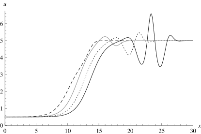
Figure 8: Numerical solution of the system (20) in case when $\tau=\kappa=1,\,m_{1}=0.5,\,m_{2}=1.5,\,m_{3}=5,\,C_{2}=1,\,C_{3}=3,$ and the invariant kink-like solution (19) is taken as the Cauchý data. Successive graphs present the TW, moving from left to right

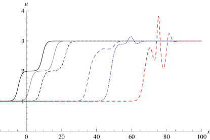
Figure 9: Numerical solution of the system (20) in case when $\tau=\kappa=1,\,\,m_{1}=1,\,m_{2}=2,\,m_{3}=3,\,C_{2}=100,\,C_{3}=0.01,$ and the invariant kink-like solution (19) is taken as the Cauchý data. Successive graphs present the TW, moving from left to right

Numerical simulations purposed at studying the evolution of soliton-like solutions to the equation (1) show, that these solutions are rather unstable. In a number of numerical simulations, performed with different functions $g(u)$ and $\kappa(u)$, we had encountered three types of instabilities destroying the TW solution. The first type is connected with the instability of the constant asymptotic solution. Two other types are manifested in either fading or blowing-up of solution in finite time. Since this behavior is rather typical, let us illustrate it on the example of the solitary wave solutions of the equation

$$\tau\,u_{tt}+u_{t}+u\,u_{x}=\kappa\,u_{x\,x}+\gamma\,u\,\left(1-u^{2}\right)$$ (22)

considered in paper [20]. The factorized system

$$\begin{array}[]{l}\Delta\,U^{\prime}(z)=\Delta\,W(z),\\ \Delta\,W^{\prime}(z)=\left[s-U[z]\right]\,W+U[z]\,\left(1-U^{2}[z]\right),\end{array}$$ (23)

obtained via the substitution (2), possesses the homoclinic solutions attained through two bifurcations. The first one is the Hopf bifurcation taking place when $\gamma\,\Delta>0$ [21], and the parameter $s$ is close to the unity. The second one is non-local and is captured numerically.

In both possible cases, i.e., when for $\gamma$ and $\Delta$ are simultaneously positive or negative, variation of velocity $s$ near the unit value leads to the appearance of homoclinic loop corresponding to the soliton-like solution.

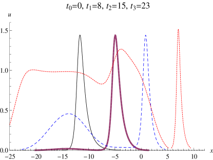
Figure 10: Numerical solution of the system (22) performed with $\tau=2,\,\kappa=1,\,\,\gamma=1$, when the invariant soliton-like solution obtained by solving the system (23) is taken as the Cauchý data.

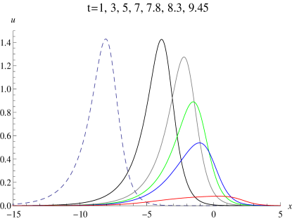
Figure 11: Numerical solution of the system (22) with $\tau=0.25,\,\kappa=1,\,\,\gamma=-1\,\,(M=0.71)$ when the invariant soliton-like solution obtained by solving the system (23) is taken as the Cauchý data.

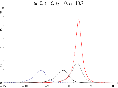
Figure 12: Numerical solution of the system (22) in case when the invariant soliton-like solution obtained by solving the system (23) with $\tau=1,\,\kappa=2,\,\,\gamma=-1\,\,(M=1.004)$ is taken as the Cauchý data.

Numerical integration of the Cauchy problem for (22) with the soliton-like solution taken as the Cauchy data, performed with the following values of the parameters $\tau=2,\,\kappa=1,\,\gamma=1,\,\,s=0.84912$ (when both $\Delta$ and $\gamma$ are positive), reveals that the initial solitary wave evolves in a self-similar mode for some time, but finally is destroyed as a result of instability of the asymptotic state, Fig. 10. Let us note, that the instability of the stationary asymptotic solution $u=U_{0}=0$ is confirmed by inspection of the formula (13). Evolution of the soliton-like solution appearing in two other cases depends on the magnitude of the characteristic number $M={u_{max}}/{C_{0}}$, where $u_{max}$ is the maximal amplitude of the initial perturbation, $C_{0}=\sqrt{\kappa/\tau}$ is the acoustic waves’ characteristic velocity. We call $M$ the ”Mach number”, since it plays the analogous role, as the parameter known under this name plays in the theory of supersonic flows. Indeed, if $M<1$, then the initial solitary wave vanishes to zero, Fig. 11. Let us note, that we deal in this case with the destruction mechanism, which is completely different from the convenient dispersion. The TW evolves for a while in self-similar mode, but at some instant its amplitude is subjected to the drastic decrease so that the wave pack completely vanishes in finite time.

When $M>1$ then the evolution of the solitary wave ends with the blow-up regime appearance, Fig. 12. We would like to mention in this place, that such a strong dependence of solutions of the nonlinear hyperbolic-type equation similar to (1) upon the ”Mach number” was noted for the first time in paper [18].

6 Discussion

Thus in this work qualitative and numerical investigations of the TW solutions of the system (1) have been performed, with special attention paid to the behavior of the kink-like and soliton-like solutions. On the basis of the results obtained, we can state that incorporation of the second-derivative with respect to time does not lead to drastic change of the situation taking place in the case of the classical convection-reaction-diffusion equation, for which a monotonic kink-like solution is stable if both of the constant asymptotic solutions are stable, while the soliton-like solution is always unstable. In fact, the situation in the case of the equation (1) is not so clear, for the Sturm Oscillation Theorem cannot be directly applied when $g(u)$ and $\kappa(u)$ are nontrivial functions. Yet in the situation when both $\kappa(u)$ and $g(u)$ are constant, and we can formulate the variational problem in the Sturm-Liouville form, the results of qualitative analysis show, that an extra inequality should be fulfilled in order that the kink-like solution be stable. Under the same conditions, any soliton-like solution proves to be unstable, as this is the case when $\tau=0.$ Numerical experiments performed with different $\kappa(u)$, $g(u)$ and $f(u)$ for which the source equation possesses the solitary-wave solutions (taken as the Cauchy data), reveal the instability in the wide range of the parameters’ values. They evidence that solitons, compactons, and shock waves appearing in the class of the generalized convection-reaction-diffusion equations remain unstable in the case of positive $\tau$.

References

- [1] Barenblatt G. I., Similarity, Self-similarity and Intermediate Asymptotics, Consultants Bureau, New York, 1979.
- [2] Samarskii A., Galaktionov V.,Kurdiumov A., Mikhailov A., Blow-up in Quasilinear Parabolic Equations, Walter de Gruyter, NY, 1995.
- [3] Danilov V., Maslov V., and Volosov K., Mathematical Modelling of heat and Mass Transfre Processes, Kluver Academic Publ., Dordrecht, Boston, 1995.
- [4] Gilding B. H., Kersner R., Travelling Waves in Nonlinear Diffusion-Convection-Reaction, Birkhauser, 2004.
- [5] Richards L. A., Capillarity conduction of liquids through porous medium, Physica, 1 (1931), 318–333.
- [6] Zeldovich Ya., Theory of Flame Propagation, National Advisory Committee for Aeronautics Technical Memorandum 1282 (1951), 39 pp.
- [7] Kolmogorov A., Petrovskii I., Piskunoff N., Dynamics of Curved Fronts (edited by P.Pelce), Academic Press, Boston, 1988, pp. 105-130.
- [8] Murray J. D., Mathematical Biology, Springer-Verlag, Berlin, 1989.
- [9] Kawahara T., Tanaka M., Phys. Letters A, vol. 97 (1983), 311-314.
- [10] Galaktionov V., Diff. Int. Equations, vol. 3 (1990), 863-874.
- [11] Clarkson P., Mansfields E., Physica D, vol. 70 (1993), 250-288.
- [12] Cherniha R., J. Math. Anal. Appl., vol. 326 (2007), 783-799.
- [13] Barannyk A., Yurik I., Proc. of the Institute of Mathematics of NAS of Ukraine, vol. 50, Part I (2004), 29-33.
- [14] Nikitin A., Barannyk T., Central European Journ. of Mathematics, vol. 2 (2005), 840-858.
- [15] Ivanova N., Dynamics of PDE, vol. 5, No. 2 (2008), 139-171.
- [16] , Joseph D.D., Preziozi, L., Review of Modern Physics, vol. 61, No. 1 (1989), 41-73.
- [17] Makarenko A., Rep. Math. Physics, vol. 46, No. 1/2 (2000), 183-190.
- [18] Makarenko A.S., Moskalkov M., Levkov S., Phys Lett. A, vol. 23 (1997), 391-397
- [19] Kar S., Banik S.K., Ray Sh., Jornal of Physics A: Mathematical and Theoretical, vol. 36, No. 11 (2003), 2771-2780.
- [20] Vladimirov V., Kutafina E., Rep. Math. Physics, vol. 54 (2004), 261–271.
- [21] Vladimirov V., Kutafina E., Rep. Math. Physics, vol. 56 (2005), 421-436.
- [22] Vladimirov V., Kutafina E., Rep. Math. Physics, vol. 58 (2006), 465-476.
- [23] Vladimirov V., Ma̧czka Cz., Rep. Math. Physics, vol. 60 (2007), 317-328.
- [24] Kutafina E., Journ. of Nonlinear Mathematical Physics, vol. 16 (2009), 517-519.
- [25] Vladimirov V., Ma̧czka Cz., Rep. Math. Physics, vol. 65 (2010), 141-156.
- [26] Vladimirov V., Wave patterns within the generalized convection-reaction-diffusion equation, arXiv:0911.2759v1 [nlin.PS]
- [27] Guckenheimer J., Holmes Ph., Nonlinear Oscillations, Dynamical Systems and Bifurcations of Vector Fields, Springer, NY, 1987.
- [28] Hassard , Kazarinoff, Wan Theory and Applications of the Hopf Bifurcation, Springer, NY, 1981.
- [29] Vladimirov, Compacton-like solutions of some nonlocal hydrodynamic-type models, Proceedings of the IV Workshop ”Group Analysis of Differential Equations and Symmetry and Integral Systems, October 25-30, 2008, Protaras, Cyprus”, pp. 210-225.
- [30] Maurin K., Analysis, PWN Publ., Warsaw, 1974.
- [31] Simon B., Sturm Oscillation and Comparison Theorems, arXiv:math/0311049 v1 [math. SP]
- [32] Idris I., Biktashev V.N., An analytical approach to initiation of propagating fronts, arxiv:0809.0252v1 [nlin.PS]
- [33] Vladimirov V., Ma̧czka Cz., Chaos, Solitons & Fractals, vol. 44 (2011), 677-684.