Einstein-Podolsky-Rosen-like correlation on a coherent-state basis
and inseparability of two-mode Gaussian states

Abstract

The strange property of the Einstein-Podolsky-Rosen (EPR) correlation between two remote physical systems is a primitive object on the study of quantum entanglement. In order to understand the entanglement in canonical continuous-variable systems, a pair of the EPR-like uncertainties is an essential tool. Here, we consider a normalized pair of the EPR-like uncertainties and introduce a state-overlap to a classically correlated mixture of coherent states. The separable condition associated with this state-overlap determines the strength of the EPR-like correlation on a coherent-state basis in order that the state is entangled. We show that the coherent-state-based condition is capable of detecting the class of two-mode Gaussian entangled states. We also present an experimental measurement scheme for estimation of the state-overlap by a heterodyne measurement and a photon detection with a feedforward operation.

I Introduction

In the seminal paper EPR35 , Einstein, Podolsky, and Rosen (EPR) considered a pair of particles, say $A$ and $B$, that possesses perfect correlation not only in their positions $x_{A(B)}$ but also in their momentums $p_{A(B)}$. From such a correlation, one can predict either the position or the momentum of one particle with certainty by measuring the position or the momentum of the other particle, and this seemingly contradicts the canonical uncertainty relation

$$\sqrt{\langle\Delta^{2}\hat{x}\rangle\langle\Delta^{2}\hat{p}\rangle}\geq|[\hat{x},\hat{p}]|/2=:C,$$ (1)

where $\Delta\hat{O}:=\hat{O}-\langle\hat{O}\rangle$. This type of seeming inconsistency between the quantum correlation and the canonical uncertainty relation is often termed as the EPR paradox and has been providing insightful aspects on foundations of quantum physics and theory of entanglement Horo09 ; Ades07 ; gtphysrep ; EPR-para .

The EPR-type correlation is normally described by the variances of the EPR-type operators $\hat{x}_{A}-\hat{x}_{B}$ and $\hat{p}_{A}+\hat{p}_{B}$, and the measured uncertainties can be a signature of quantum entanglement. Duan et al., Duan00 have introduced the EPR-like operators $\hat{X}:=|a|\hat{x}_{A}-\frac{1}{a}\hat{x}_{B}$ and $\hat{P}^{\prime}:=|a|\hat{p}_{A}+\frac{1}{a}\hat{p}_{B}$ with a real number $a$, and presented an inseparable condition associated with the total variance of the operators: A bipartite state is entangled if it violates the inequality

$$\langle\Delta^{2}\hat{X}\rangle+\langle\Delta^{2}\hat{P}^{\prime}\rangle\geq 2(a^{2}+\frac{1}{a^{2}})C.$$ (2)

Interestingly, this condition is conducted to determine the inseparability of two-mode Gaussian states. To be specific, for any given entangled two-mode Gaussian state, there exists a proper local Gaussian-unitary transformation and a parameter $a$ so that the inequality of Eq. (2) is violated. Its implication is that the origin of the inseparability of two-mode Gaussian states lies on the strength of the EPR-like correlation.

A quantum state on a bipartite system $AB$ is called separable if its density operator can be written in the convex sum form of the products of local density operators as $\rho_{AB}=\sum_{i}p_{i}(\rho_{i})_{A}\otimes(\sigma_{i})_{B}$ where $(\rho_{i})_{A}$ and $(\sigma_{i})_{B}$ are local density operators of the system $A$ and $B$, respectively, and $p_{i}$ is a probability distribution that satisfies $p_{i}\geq 0$ and $\sum p_{i}=1$. A quantum state is said to be entangled if it is not separable. The separable density operator preserves its positivity under the transpose of its local density matrix. This property of positive partial transposition cannot hold for many of entangled density operators, and non-positivity of the partial transposition is a signal of entanglement Peres . An important fact is that the class of Gaussian entangled states belongs to the entanglement with non-positive partial transposition Simon00 ; Giedke01 . It is shown that many of known separable conditions concerning the continuous-variable states, which include Eq. (2), can be derived by using partial transposition for moments of the annihilation operators and the creation operators SV ; Mira09 .

In quantum optics, the canonical variables correspond to the phase-space quadratures of optical modes, and their statistics can be measured by the homodyne measurement. This enables us to determine the moments of annihilation and creation operators in experiments. The homodyne measurement is a standard Gaussian-measurement and plays a central role in the continuous-variable quantum information processing CV-RMP . Another important Gaussian measurement is the heterodyne (double homodyne) measurement. It measures the complex amplitude $\alpha$ of an optical coherent state $\left|\alpha\right\rangle$ and gives the projection probability to the coherent state $\left\langle\alpha\right|\rho\left|\alpha\right\rangle$. The canonical quadratures and coherent-state amplitudes provide similar phase-sensitive information of the optical modes, and both of them are thought to be useful to observe the properties of Gaussian states. There have been several approaches to suggest the relation between heterodyne statistics and entanglement mainly associated with the transmission of coherent states GroInf . It might be also insightful to consider the separablity problems related to the phase-space distribution Bana99 ; Mar09 ; Mira10 . However, their implication with respect to the EPR-like correlation has little been discussed.

Recently, a separable condition with the state-overlap to the Gaussian distributed phase-conjugate pairs of coherent states was derived namiki11 . It states that any separable state has to satisfy

$$\left\langle\int p_{\lambda}(\alpha)\left|\alpha\right\rangle\left\langle\alpha\right|\otimes\left|\sqrt{\eta}\alpha^{*}\right\rangle\left\langle\sqrt{\eta}\alpha^{*}\right|d^{2}\alpha\right\rangle\leq\frac{\lambda}{1+\lambda+\eta},$$ (3)

where $p_{\lambda}(\alpha):=\frac{\lambda}{\pi}\exp(-\lambda|\alpha|^{2})$ and $\eta,\lambda\geq 0$. Since the state-overlap in the left-hand side is written in terms of the projections to the coherent states, it can be estimated by the statistics of the heterodyne measurement. The condition of Eq. (3) was formulated for the quantum benchmark problem Bra00 ; Ham05 ; namiki07 ; namiki08 ; Namiki11APB ; namiki11 ; Has08 ; Has09 ; Cal09 ; Owari08 ; Adesso08 ; Guta10 ; Has10 ; Takano08 ; Kil10 ; Kil11 ; Namiki12R , however, its utility and significance for the separability problem have little been discussed.

In this paper we investigate the properties of the overlap condition of Eq. (3) for the separability problem. We argue that the state-overlap is a form of the EPR-like correlation in a coherent-state basis. It is shown that the separable condition with the overlap and the separable condition with the EPR-like uncertainties can be formulated in parallel, and the violation of the separable conditions can be interpreted as a phenomenon to infer the EPR paradox. For the Gaussian states given in a standard form of the covariance matrix we find a simple embrace relation between the separable conditions. This relation provides a geometric proof that the overlap condition can be conducted to determine the inseparability of two-mode Gaussian states. We also consider experimental measurement schemes to detect the state-overlap.

This paper is organized as follows. We introduce a limitation of the phase-space localization as a sort of the canonical uncertainty relation in Sec. II. We derive the separable condition with the EPR-like uncertainties and investigate its properties in Sec. III. We derive the overlap separable condition and discuss its properties in Sec. IV. Then, we address the utility of the overlap condition for Gaussian states in Sec. V. We present the experimental scheme in Sec. VI. We conclude this paper in Sec. VII.

II Uncertainty relation and Phase-space Localization

An intuitive interpretation of the canonical uncertainty relation in Eq. (1) is that the quantum state is located on the phase space with a finite volume [See FIG. 1(a)]. When the volume is measured in terms of the uncertainty product $\sqrt{\langle\Delta^{2}\hat{x}\rangle\langle\Delta^{2}\hat{p}\rangle}$, it cannot be smaller than the limit determined by the canonical commutation relation, i.e., $\sqrt{\langle\Delta^{2}\hat{x}\rangle\langle\Delta^{2}\hat{p}\rangle}\geq|[\hat{x},\hat{p}]|/2$. The standard deviation describes typical width of the phase-space distribution and thus the uncertainty product indicates a degree of localization of the phase-space distribution. Here, we consider another measure of the phase-space localization and present another form of the physical limitation.

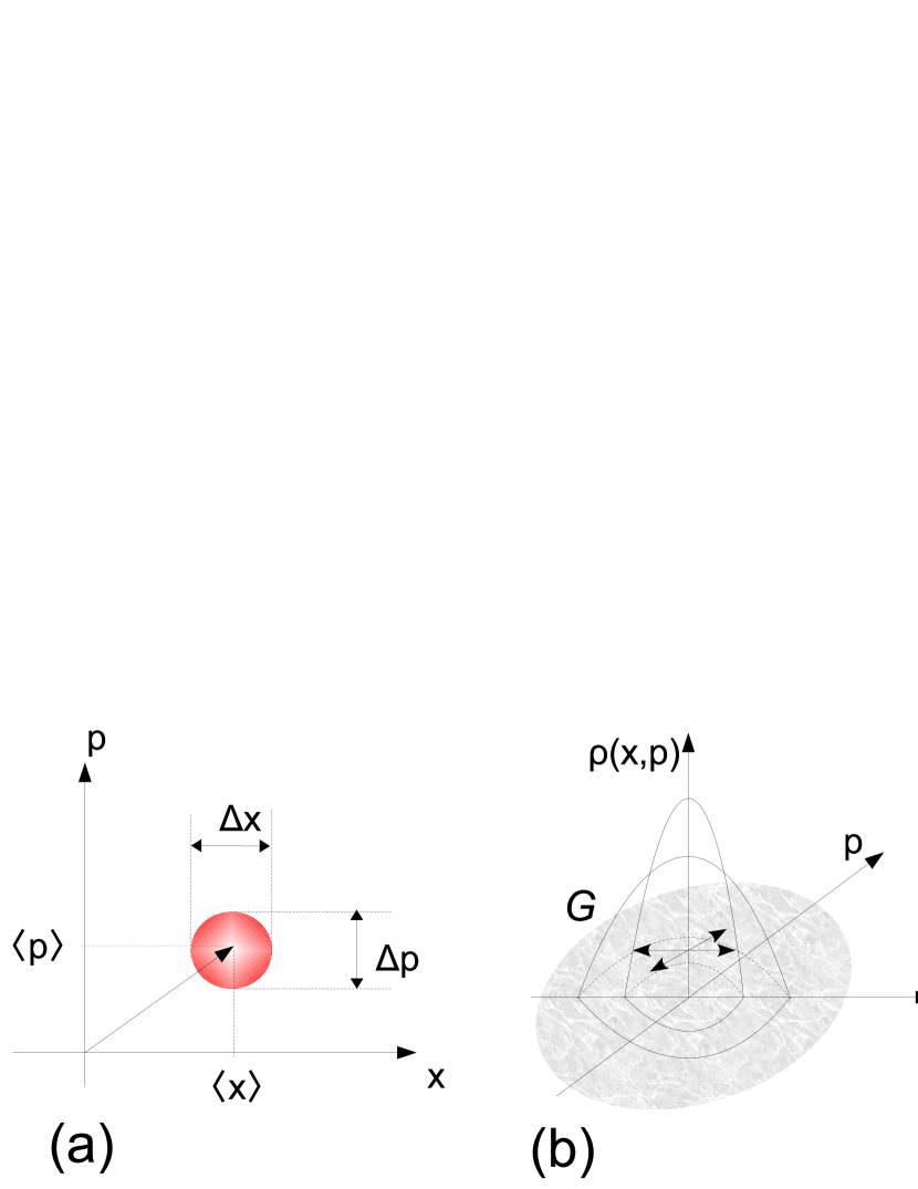
Figure 1: (Color online) The uncertainty relation gives a limitation on the localization in the phase space. (a) A physical state is spread in the phase space so that its volume of ${\Delta x}{\Delta p}$ is no smaller than the minimum uncertainty product of $|[\hat{x},\hat{p}]|/2$ due to the canonical uncertainty relation. (b) Another measure of the phase-space localization can be given by the convolution between the state distribution $\rho(x,p)$ and a localized distribution function $G$ on the phase space. The value of the convolution designates the concentration of the state distribution at the peak of the function $G$.

Let us consider the density operator of a thermal state

$$\hat{G}_{\lambda} := \int p_{\lambda}(\alpha)\left|\alpha\right\rangle\left\langle\alpha\right|d^{2}\alpha$$ (4)

$$= \frac{\lambda}{1+\lambda}\sum_{n=0}^{\infty}\left(\frac{1}{1+\lambda}\right)^{n}\left|n\right\rangle\left\langle n\right|.$$

Here we use the standard notation for the number state $\left|n\right\rangle$ and the coherent state $\left|\alpha\right\rangle=\sum_{n=0}^{\infty}e^{-|\alpha|^{2}/2}\alpha^{n}\left|n\right\rangle/\sqrt{n!}$. The phase-space distribution of the thermal state is an isotropic Gaussian distribution and peaked at the origin of the phase space $\alpha=0$ [See FIG. 1(b)]. The expectation value of the thermal state $\langle\hat{G}\rangle_{\rho}:={\textrm{Tr}}{\hat{G}\rho}=\lambda\int Q_{\rho}(\alpha)e^{-\lambda|\alpha|^{2}}d^{2}\alpha$ is a Gaussian convolution of the Husimi-$Q$ function $Q_{\rho}(\alpha):=\left\langle\alpha\right|\rho\left|\alpha\right\rangle/\pi$. It suggests how strong the probability distribution is concentrated around the origin. Hence, it is likely that the expectation value is maximized by the state which has a sharply peaked $Q$ function at $\alpha=0$. However, we cannot make the width of the $Q$ function arbitrarily small, and thus $\langle\hat{G}_{\lambda}\rangle$ has an upper bound. This upper bound offers another form of the physical limitation on the degree of the phase-space localization. From the second line of Eq. (4), an upper bound of $\langle\hat{G}\rangle$ is given by the maximum eigenvalue of the thermal state $\|\hat{G}_{\lambda}\|$ as

$$\langle\hat{G}_{\lambda}\rangle\leq\|\hat{G}_{\lambda}\|=\frac{\lambda}{1+\lambda}.$$ (5)

This relation serves as a sort of the uncertainty relation, namely, one cannot localize the physical state on the phase space so that the expectation value $\langle\hat{G}\rangle$ surpasses the physical limit $\|\hat{G}_{\lambda}\|$. We refer to $\langle\hat{G}_{\lambda}\rangle_{\rho}={\textrm{Tr}}\hat{G}_{\lambda}\rho$ as the $\lambda$-localization of a density operator $\rho$. The equality of Eq. (5) can be achieved by the vacuum state $\left|0\right\rangle$ and the vacuum state is the maximally $\lambda$-localized state. Since, the $\lambda$-localization is an overlap between a given state and the thermal state, it represents the probability of finding the states in the thermal distribution.

In order to see an intuitive connection between the uncertainty product and the $\lambda$-localization, let us consider the case where the $Q$ function has a single peak at the origin. Let $\delta x$ and $\delta p$ be the width of the $Q$ function along the real $x$ direction and the imaginary $p$ direction, respectively. Then, the normalization condition $1=\int Q_{\rho}(\alpha)d^{2}\alpha\simeq Q_{\rho}(0)\delta x\delta p$ implies $Q_{\rho}(0)\simeq(\delta x\delta p)^{-1}$. Hence, for sufficiently large $\lambda$, we have $\langle\hat{G}_{\lambda}\rangle=\lambda\int Q_{\rho}(\alpha)e^{-\lambda|\alpha|^{2}}d^{2}\alpha\simeq\pi Q_{\rho}(0)\simeq\pi(\delta x\delta p)^{-1}$, namely, the $\lambda$-localization is proportional to the inverse of the uncertainty product, in a certain limit.

III Separable conditions with the EPR-like uncertainties

In this section, we derive a separable condition with a normalized EPR-like uncertainty product using partial transposition for the canonical uncertainty relation. This separable condition is called the product condition Reid89 ; Tan99 ; Gio03 ; Hyl06 and has a simple embrace relation to the sum separable condition of Eq. (2). In contrast to the sum condition, any point of the separable boundary of the product condition can be achieved by the product of the squeezed states. It is shown that the maximum of the EPR-like correlation can be achieved by a two-mode squeezed state (TMSS).

We start with the canonical uncertainty relation

$$\langle\Delta^{2}\hat{x}\rangle\langle\Delta^{2}\hat{p}\rangle\geq\left(\frac{|[\hat{x},\hat{p}]|}{2}\right)^{2}=C^{2}.$$ (6)

By introducing an ancilla system $B$ and applying a beamsplitter transformation $(\hat{x}_{A},\hat{p}_{A})\to(u\hat{x}_{A}-v\hat{x}_{B},u\hat{p}_{A}-v\hat{p}_{B})$ we have

$$\langle\Delta^{2}\left(u\hat{x}_{A}-v\hat{x}_{B}\right)\rangle\langle\Delta^{2}\left(u\hat{p}_{A}-v\hat{p}_{B}\right)\rangle\geq C^{2},$$ (7)

where we assign the index $A$ for the original system and assume that the real parameters $(u,v)$ satisfy the relation $u^{2}+v^{2}=1$. When we make the replacement $p_{B}\to-p_{B}$ Aga05 we have a product separable condition Gio03 ; Hyl06 ; SV

$$\langle\Delta^{2}\left(u\hat{x}_{A}-v\hat{x}_{B}\right)\rangle\langle\Delta^{2}\left(u\hat{p}_{A}+v\hat{p}_{B}\right)\rangle\geq C^{2}.$$ (8)

The replacement corresponds to the transposition of the system $B$ with respect to the number basis (see the below proof). The left-hand side of Eq. (8) is a normalized EPR-like uncertainty product so that it becomes a normal uncertainty product for the canonical variables under the partial transposition as in Eq. (7). Since the partial transposition is not a physical transformation, it is no reason to consider that Eq. (8) holds for all physical states. We can show that separable states cannot violate this inequality as follows:

Proof. — Let us write $\hat{X}:=u\hat{x}_{A}-v\hat{x}_{B}$, $\hat{P}:=u\hat{p}_{A}-v\hat{p}_{B}$, and the partial transposition, which transposes the system $B$ with respect to the number basis,

$$\Gamma:(|l\rangle\langle m|\otimes|j\rangle\langle k|)\to(|l\rangle\langle m|\otimes|k\rangle\langle j|).$$ (9)

For product states, we can write the expectation value of the partial transposed observable $\hat{O}$ as $\langle\Gamma[\hat{O}]\rangle_{\phi\otimes\varphi}={\textrm{Tr}}[\Gamma[\hat{O}]\left|\phi\right\rangle\left\langle\phi\right|\otimes\left|\varphi\right\rangle\left\langle\varphi\right|]={\textrm{Tr}}[\hat{O}\Gamma(\left|\phi\right\rangle\left\langle\phi\right|\otimes\left|\varphi\right\rangle\left\langle\varphi\right|)]={\textrm{Tr}}(\hat{O}\left|\phi\right\rangle\left\langle\phi\right|\otimes\left|\varphi^{*}\right\rangle\left\langle\varphi^{*}\right|)=\langle\hat{O}\rangle_{\phi\otimes\varphi^{*}}$. Here we defined the conjugate state by $\left|\varphi^{*}\right\rangle:=\sum_{n=0}^{\infty}\langle\varphi|n\rangle\left|n\right\rangle$. Since the off-diagonal elements of the position operator $\hat{x}=\sqrt{C}(\hat{a}+\hat{a}^{\dagger})$ in the number basis are real we have $\Gamma[\hat{X}]=\hat{X}$. In contrast, the off-diagonal elements of the momentum operator $\hat{p}=\sqrt{C}(\hat{a}-\hat{a}^{\dagger})/i$ in the number basis are pure imaginary, and we thus have $\Gamma[\hat{P}]=u\hat{p}_{A}+v\hat{p}_{B}$. Noting that $\Gamma[\hat{P}^{2}]=(\Gamma[\hat{P}])^{2}$ and $\Gamma[\hat{X}^{2}]=(\Gamma[\hat{X}])^{2}$, we can estimate the left-hand side of Eq. (8) as $\langle\Delta^{2}(\Gamma\hat{X})\rangle_{\phi\otimes\varphi}\langle\Delta^{2}(\Gamma\hat{P})\rangle_{\phi\otimes\varphi}=\langle\Delta^{2}\hat{X}\rangle_{\phi\otimes\varphi^{*}}\langle\Delta^{2}\hat{P}\rangle_{\phi\otimes\varphi^{*}}\geq\min_{\phi\otimes\varphi}\left\{\langle\Delta^{2}\hat{X}\rangle_{\phi\otimes\varphi}\langle\Delta^{2}\hat{P}\rangle_{\phi\otimes\varphi}\right\}\geq(|[\hat{X},\hat{P}]|/2)^{2}$ for any product state. Hence, for any separable state $\rho_{s}=\sum_{i}p_{i}\left|\phi_{i}\right\rangle\left\langle\phi_{i}\right|\otimes\left|\varphi_{i}\right\rangle\left\langle\varphi_{i}\right|$ we have

$$\langle\Delta^{2}(\Gamma\hat{X})\rangle_{\rho_{s}}\langle\Delta^{2}(\Gamma\hat{P})\rangle_{\rho_{s}}$$ (10)

$$= (\sum_{i}p_{i}\langle\Delta^{2}\hat{X}\rangle_{\phi_{i}\otimes\varphi_{i}^{*}})(\sum_{j}p_{j}\langle\Delta^{2}\hat{P}\rangle_{\phi_{j}\otimes\varphi_{j}^{*}})$$

$$\geq \left(\sum_{j}p_{j}\sqrt{\langle\Delta^{2}\hat{X}\rangle_{\phi_{j}\otimes\varphi_{j}^{*}}\langle\Delta^{2}\hat{P}\rangle_{\phi_{j}\otimes\varphi_{j}^{*}}}\right)^{2}$$

$$\geq (|[\hat{X},\hat{P}]|/2)^{2}=C^{2}.$$

From the second line to the third line, we set $a_{j}=\sqrt{p_{j}\langle\Delta^{2}\hat{X}\rangle_{\phi_{j}\otimes\varphi_{j}^{*}}}$, $b_{j}=\sqrt{p_{j}\langle\Delta^{2}\hat{P}\rangle_{\phi_{j}\otimes\varphi_{j}^{*}}}$ and use the Schwarz inequality $|\vec{a}|^{2}|\vec{b}|^{2}\geq|\vec{a}\cdot\vec{b}|^{2}$. $\blacksquare$

An important implication of the product separable condition of Eq. (8) is that the EPR-like correlation cannot be stronger than the canonical uncertainty limit without entanglement. As was shown in the proof, the EPR-like uncertainty product for a product state can be mapped into the canonical uncertainty product for its conjugat state when the EPR-like operators are normalized so that their partial transpositions form a pair of the canonical observables. From this normalization, the phase-space localization can be directly associated with the EPR-paradox, namely, the seeming violation of the limitation on the phase-space localization verifies the existence of entanglement.

Dividing both sides of Eq. (2) by $(a^{2}+1/a^{2})$ we have a normalized sum condition

$$\langle\Delta^{2}\left(u\hat{x}_{A}-v\hat{x}_{B}\right)\rangle+\langle\Delta^{2}\left(u\hat{p}_{A}+v\hat{p}_{B}\right)\rangle\geq 2C,$$ (11)

where we set

$$(u,v)=\frac{1}{\sqrt{a^{2}+a^{-2}}}(|a|,a^{-1}).$$ (12)

This sum condition of Eq. (11) can be also obtained by taking the square root on both sides of Eq. (8) and using the relation $\langle\Delta^{2}\left(u\hat{x}_{A}-v\hat{x}_{B}\right)\rangle+\langle\Delta^{2}\left(u\hat{p}_{A}+v\hat{p}_{B}\right)\rangle\geq 2\sqrt{\langle\Delta^{2}\left(u\hat{x}_{A}-v\hat{x}_{B}\right)\rangle\langle\Delta^{2}\left(u\hat{p}_{A}+v\hat{p}_{B}\right)\rangle}$. From this derivation we can see that the inequality of Eq. (8) is automatically violated if the inequality of Eq. (11) is violated. This suggests that the product condition of Eq. (8) is better to detect entanglement than the sum condition of Eq. (11). To show the advantage of the product condition more clearly, let us write the normalized uncertainties of the EPR-like operators as

$$U: = {\langle\Delta^{2}\left(u\hat{x}_{A}-v\hat{x}_{B}\right)\rangle}/C$$

$$V: = {\langle\Delta^{2}\left(u\hat{p}_{A}+v\hat{p}_{B}\right)\rangle}/C.$$ (13)

Then, the product separable condition of Eq. (8) leads to

$$UV\geq 1,$$ (14)

and the sum separable condition of Eq. (11) leads to

$$U+V\geq 2.$$ (15)

The embrace relation between Eqs. (14) and (15) can be directly observed in FIG. 2. Since there is no separable state below the curve $UV=1$ (gray regime of FIG. 2), the states located on the boundary of Eq. (11) should be entangled except for the single point $(U,V)=(1,1)$. As a result, the sum condition fails to notice the entangled states located in the area enclosed by the two curves $UV=1$ and $U+V=2$. As a separable state located on the boundary of Eq. (14), we can find the product of the squeezed states $\hat{S}_{A}\otimes\hat{S}_{B}|0,0\rangle_{AB}$ where $\hat{S}$ stands for the squeezing operator.

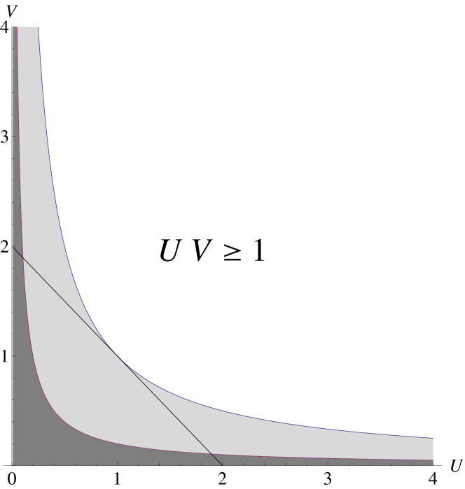
Figure 2: (Color online) Relation between the inseparability and the normalized EPR-like uncertainties $U$ and $V$ in Eq. (13). The product condition of Eq. (8) [Eq. (14)] implies that any state is entangled if its location $(U,V)$ is below the inverse proportional curve $UV=1$ (gray regime). On the other hand, for any point of this curve one can find a corresponding separable state (See main text). The violation of the sum condition of Eq. (11) [Eq. (15)] occurs for the states located below the straight line $U+V=2$, and the entangled states detected by the sum condition belong to a subset of the entangled states detected by the product condition. The dark gray regime is physically unaccessible due to the global canonical uncertainty relation of Eq. (16). In this figure we set $|u^{2}-v^{2}|^{2}=0.2$ specifically so that the physical boundary is given by $UV=0.2$.

Note that the physical limitation for the EPR-like uncertainty product is give by

$$\langle\Delta^{2}\left(u\hat{x}_{A}-v\hat{x}_{B}\right)\rangle\langle\Delta^{2}\left(u\hat{p}_{A}+v\hat{p}_{B}\right)\rangle$$

$$\geq \left(\frac{|[u\hat{x}_{A}-v\hat{x}_{B},u\hat{p}_{A}+v\hat{p}_{B}]|}{2}\right)^{2}=(u^{2}-v^{2})^{2}C^{2}.$$

In terms of $U$ and $V$, it can be expressed as

$$UV\geq|u^{2}-v^{2}|^{2}.$$ (16)

This inequality is saturated by the TMSS

$$|\psi_{\zeta}\rangle_{AB} = \sqrt{1-|\zeta|^{2}}\sum_{n=0}^{\infty}\zeta^{n}|n\rangle_{A}|n\rangle_{B},$$ (17)

with $\zeta=v/u<1$. We can observe that the TMSS is located at $(U,V)=({u^{2}-v^{2}},{u^{2}-v^{2}})$ on the $U$-$V$ plane and that the physical boundary of Eq. (16) can be covered by the state $\hat{S}_{A}\otimes\hat{S}_{B}|\psi_{\zeta}\rangle_{AB}$ similar to the case that the product of the squeezed states covers the separable boundary of Eq. (14). Noting the relation $U+V\geq 2\sqrt{UV}\geq 2({u^{2}-v^{2}})$, we can see that the physically possible minimum of the sum $U+V$ is also achieved by the same TMSS located at $({u^{2}-v^{2}},{u^{2}-v^{2}})$.

The fact that the product condition is better than the sum condition is generally stressed in Hyl06 ; Gio03 and the results of Refs. Hyl06 ; SV ; Gio03 essentially include the condition of Eq. (8) although the EPR-like operators are not normalized so that their partial transpositions form a pair of the canonical variables. For the case of $|u|=|v|$, the separable condition of Eq. (8) is derived in Tan99 ; Manc02 ; Aga05 . From the superiority of the product condition and the fact Duan00 ; Simon00 that any Gaussian entangled state can be detected by the violation of the sum condition, it is concluded Gio03 that any two-mode Gaussian entangled state can be detected by the violation of the product condition. There is an approach to consider that the sum condition is a condition for a quadratic Hamiltonian, thereby a separable condition on the variance of the normalized Hamiltonian is derived namiki10 .

To estimate the left-hand sides of Eqs. (8) and (11) in the experiments, one may perform the joint quadrature measurement of $\hat{x}_{A}\hat{x}_{B}$ and $\hat{p}_{A}\hat{p}_{B}$ (For the estimation of the covariance matrix of the two-mode state, it requires the measurement of $\hat{x}_{A}\hat{p}_{B}$ and $\hat{p}_{A}\hat{x}_{B}$, additionally). The measured homodyne statistics of $\hat{x}_{A}\hat{x}_{B}$ and $\hat{p}_{A}\hat{p}_{B}$ give the six variances $\{\langle\Delta^{2}\hat{x}_{A}\rangle$, $\langle\Delta^{2}\hat{x}_{B}\rangle$, $\langle\Delta^{2}\hat{p}_{A}\rangle$, $\langle\Delta^{2}\hat{p}_{B}\rangle$, $\langle\Delta\hat{x}_{A}\Delta\hat{x}_{B}\rangle$, $\langle\Delta\hat{p}_{A}\Delta\hat{p}_{B}\rangle\}$. Then, the left-hand side of Eq. (8) can be determined for any set of $(u,v)$. In practice, it is better to use the set of the parameters $(u,v)$ so that the left-hand side of Eq. (8) becomes as small as possible. The minimum can be readily found by setting $(u,v)=(\cos{\theta},\sin{\theta})$ and plotting the left-hand side of Eq. (8) as a function of $\theta$. The parameter $\theta$ corresponds to the effect of the global rotation by the beamsplitter transformation. Although the joint squeezing $\hat{S}_{A}\otimes\hat{S}_{B}$ belongs to the set of local operations, it is not easy to access experimentally. In turn, to achieve the boundary of the product condition, the sum condition requires additional local squeezing operations. This suggests actual experimental advantage to use the product condition in place of the sum condition.

Note that the left-hand side of Eq. (11) becomes a quadratic form of $\vec{u}:=(u,v)^{t}$ as $\vec{u}^{t}(M_{x}+M_{p})\vec{u}$ where

$$M_{x}: = \left(\begin{array}[]{cc}\langle\Delta^{2}\hat{x}_{A}\rangle&-\langle\Delta\hat{x}_{A}\Delta\hat{x}_{B}\rangle\\ -\langle\Delta\hat{x}_{A}\Delta\hat{x}_{B}\rangle&\langle\Delta^{2}\hat{x}_{B}\rangle\\ \end{array}\right)$$ (20)

$$M_{p}: = \left(\begin{array}[]{cc}\langle\Delta^{2}\hat{p}_{A}\rangle&\langle\Delta\hat{p}_{A}\Delta\hat{p}_{B}\rangle\\ \langle\Delta\hat{p}_{A}\Delta\hat{p}_{B}\rangle&\langle\Delta^{2}\hat{p}_{B}\rangle\\ \end{array}\right).$$ (23)

Hence, the minimum of the left-hand side of Eq. (11) is given by the minimum eigenvalue of the matrix $M_{x}+M_{y}$. The minimum plays an important role in Refs. Mar09 ; Fijikawa09 . By using the matrices of Eq. (23), the left-hand sides of Eq. (8) can be expressed in a compact form $(\vec{u}^{t}M_{x}\vec{u})(\vec{u}^{t}M_{p}\vec{u})$.

IV separable condition with the coherent-state-based EPR-like correlation

In this section we use the partial transposition for the limitation on the $\lambda$-localization of Eq. (5), and derive the overlap separable condition corresponding to Eq. (3). It determines the strength of the EPR-like correlation in a coherent-state basis in order that the state is entangled. The maximal correlation on this basis is also obtained by a TMSS.

Let us consider the following positive operator

$${\hat{G}_{\lambda}^{\prime}}: = \hat{R}\hat{G}_{\lambda}\otimes\left|0\right\rangle\left\langle 0\right|\hat{R}^{\dagger}$$ (24)

$$= \int p_{\lambda}(\alpha)\left|v\alpha\right\rangle\left\langle v\alpha\right|\otimes\left|{u}\alpha\right\rangle\left\langle{u}\alpha\right|d^{2}\alpha,$$

where the thermal state $\hat{G}_{\lambda}$ is defined in Eq. (4) and the beamsplitter transformation $\hat{R}$ is defined through its action on the coherent state $\hat{R}\left|\alpha\right\rangle\left|0\right\rangle=\left|v\alpha\right\rangle\left|u\alpha\right\rangle$. Since the spectrum of $\hat{G}_{\lambda}^{\prime}$ is the same as the spectrum of $\hat{G}_{\lambda}$, the physical limitation for the $\lambda$-localization of Eq. (5) also holds for $\hat{G}_{\lambda}^{\prime}$ as

$$\langle\hat{G}_{\lambda}^{\prime}\rangle \leq \frac{\lambda}{1+\lambda}.$$ (25)

The equality is achieved by the product of the vacuum states $\left|0,0\right\rangle_{AB}$.

From the partial transposition of $\hat{G}^{\prime}$ and the physical limitation of Eq. (25) we obtain the overlap separable condition namiki11 :

$$\langle\Gamma\hat{G}_{\lambda}^{\prime}\rangle \leq \frac{\lambda}{1+\lambda},$$ (26)

where the partial transposition can be written as

$$\Gamma(\hat{G}_{\lambda}^{\prime})=\int p_{\lambda}(\alpha)\left|v\alpha\right\rangle\left\langle v\alpha\right|\otimes\left|u\alpha^{*}\right\rangle\left\langle u\alpha^{*}\right|d^{2}\alpha.$$ (27)

Here, the action of the partial transposition map $\Gamma$ of Eq. (9) induces the complex conjugation of the coherent-state amplitude of the second system in Eq. (24). The equality of Eq. (26) is also achieved by the product of the vacuum states $\left|0,0\right\rangle_{AB}$. We can show that the overlap condition of Eq. (26) holds for any separable state as follows:

Proof.— For any separable state $\rho_{s}$, $\Gamma[\rho_{s}]$ is a density operator. Using Eq. (25) for $\Gamma[\rho_{s}]$, we have $\langle\Gamma\hat{G}^{\prime}\rangle_{\rho_{s}}={\textrm{Tr}}(\rho_{s}\Gamma[\hat{G}^{\prime}])={\textrm{Tr}}(\Gamma[\rho_{s}]\hat{G}^{\prime})\leq\lambda/(1+\lambda)$. Hence, the violation of the condition in Eq. (26) implies that the state is entangled. $\blacksquare$

The expectation value of $\Gamma\hat{G}_{\lambda}^{\prime}$ in Eq. (27) is a weighted sum of the probability that the pair of coherent states $\left|\alpha\right\rangle_{A}\left|g\alpha^{*}\right\rangle_{B}$ is contained in the given state, where $g=u/v$ is a real number. Recalling that the complex amplitude is defined as $\alpha=x+ip$, the state-overlap $\langle\Gamma\hat{G}_{\lambda}^{\prime}\rangle$ essentially represents the strength of the EPR-like correlation so that the relations $x_{A}=gx_{B}$ and $p_{A}=-gp_{B}$ hold, simultaneously. Actually the two relations can be combined to the single expression $\alpha_{A}=g\alpha_{B}^{*}$ (See also FIG. 3). Note that we can reproduce Eq. (3) from Eq. (26) as follows. We change the variable of integration $\alpha^{\prime}=v\alpha$ and make the replacement $\lambda/v^{2}\to\lambda$ on Eq. (26). Then, we can obtain Eq. (3) by setting $\eta=\frac{u^{2}}{v^{2}}=\frac{1}{v^{2}}-1$. An expression of $\langle\Gamma\hat{G}_{\lambda}^{\prime}\rangle$ for Gaussian states and its link to the separable conditions with the EPR-like uncertainties can be found in Sec. V.

A violation of the overlap separable condition of Eq. (26) can be observed for the TMSS. From Eq. (17) and Eq. (27) we have

$$\langle\Gamma(\hat{G}_{\lambda}^{\prime})\rangle_{\psi_{\zeta}}=\frac{\lambda(1-\zeta^{2})}{u^{2}[1+\lambda/u^{2}-\zeta^{2}+(v/u-\zeta)^{2}]}.$$ (28)

If we set $\sqrt{2}u=\sqrt{2}v=1$ and $2\zeta=1$, the right-hand side of Eq. (28) becomes $3\lambda/(2+4\lambda)$. Hence, for $\lambda<1$, we can observe $\langle\Gamma(\hat{G}_{\lambda}^{\prime})\rangle_{\psi_{\zeta}}>\lambda/(1+\lambda)$. If the transformation $\Gamma$ preserved the phase-space localization, this expression would imply the violation of the physical limitation for the $\lambda$-localization of Eq. (25) as a sort of the EPR paradox. In reality, the partial transposition $\Gamma$ is not a physical transformation and it is no need to consider that the violation of Eq. (26) violates the physical limitation of Eq. (25). The paradox, in which entangled states can be “localized” beyond the limit achieved by the pair of coherent states, is essentially identical to the phenomenon that the EPR-like uncertainty product violates the canonical uncertainty limit. It might be helpful to consider that the phenomenon comes from the use of a strange way to sum the phase-space volume based on the partial transposed unit of the volume measure, in which the sign of the local momentum is inverted $p_{B}\to-p_{B}$. This inversion suggests the complex conjugation $i\to-i$ because the sign of the commutation relation is changed due to the replacement $[\hat{x},\hat{p}]\to-[\hat{x},\hat{p}]$. Such a replacement affects the coherence between the two systems and some of entangled states exhibit seemingly abnormal phase-space volume.

Figure 3: A pair of the EPR-like particles exhibits a strong positive correlation on their positions $x_{A}$ and $x_{B}$. It also exhibits a strong negative correlation on their momentums $p_{A}$ and $p_{B}$. A total deviation from the lines of $x_{B}=g^{-1}x_{A}$ and $p_{B}=-g^{-1}p_{A}$ represents the strength of the EPR-like correlation. The deviation can be directly related to the width of the correlation distribution as (a). The strength of the correlation can also be related to the intensity of the distribution as (b). The two conditions of $x_{B}=g^{-1}x_{A}$ and $p_{B}=-g^{-1}p_{A}$ are combined into the single expression $\alpha_{B}^{*}=g^{-1}\alpha_{A}$ with the complex amplitudes $\alpha_{A}=x_{A}+ip_{A}$ and $\alpha_{B}=x_{B}+ip_{B}$. This suggests another form of the EPR-like correlation in terms of the distribution intensities associated with the pairs of coherent states $\{\left|\alpha\right\rangle_{A}\left|g\alpha^{*}\right\rangle_{B}\}$.

Note that $\Gamma\hat{G}_{\lambda}^{\prime}$ of Eq. (27), as a density operator, is located at the point $(U,V)=(1,1)$ on the separable boundary of the $U$-$V$ plane as the vacuum state $\left|0\right\rangle\left|0\right\rangle$ is located at the same point (See FIG. 2). Moreover, the state obtained by applying the collective local squeezing both on A and B to $\Gamma\hat{G}_{\lambda}^{\prime}$, i.e., $\hat{S}_{A}\otimes\hat{S}_{B}\Gamma(\hat{G}_{\lambda}^{\prime})\hat{S}_{A}^{\dagger}\otimes\hat{S}_{B}^{\dagger}$ moves along the local minimum uncertainty boundary of Eq. (14) as $\hat{S}_{A}\otimes\hat{S}_{B}\left|0,0\right\rangle_{AB}$ does. We can see that $\hat{S}_{A}\otimes\hat{S}_{B}\Gamma(\hat{G}_{\lambda}^{\prime})\hat{S}_{A}^{\dagger}\otimes\hat{S}_{B}^{\dagger}$ reduces to the product of the pure squeezed states $\hat{S}_{A}\otimes\hat{S}_{B}\left|0,0\right\rangle_{AB}$ in the pure limit $\lambda\to\infty$. Although the form of the mixture shows the correlation explicitly, its EPR-like correlation is no stronger than the correlation given by the uncorrelated state $\left|0,0\right\rangle$.

As was mentioned above, the strength of the coherent-state-based EPR-like correlation $\langle\Gamma\hat{G}_{\lambda}^{\prime}\rangle$ is a state-overlap to the classically correlated state. It simply suggests the probability that the state contains the conjugate coherent-state pairs, and the separable condition of Eq. (26) gives the threshold of the pair appearance in order that the state is entangled. The maximum of the coherent-state-based EPR-like correlation $\langle\Gamma(\hat{G}_{\lambda}^{\prime})\rangle$ is given by the operator norm of $\Gamma(\hat{G}_{\lambda}^{\prime})$ as

$$\max_{\rho}\langle\Gamma(\hat{G}_{\lambda}^{\prime})\rangle_{\rho} = \|\Gamma(\hat{G}_{\lambda}^{\prime})\|$$ (29)

$$= \frac{4}{(\nu_{+}+1)(\nu_{-}+1)}$$

$$= \frac{2\lambda}{1+\lambda+\sqrt{(1+\lambda)^{2}-4u^{2}v^{2}}}$$

where we use the symplectic eigenvalues $\nu_{\pm}$ of $\Gamma(\hat{G}_{\lambda}^{\prime})$ defined in Eq. (44). This maximum value is achieved by the TMSS of Eq. (17) when we set

$$\zeta=[(1+\lambda)-\sqrt{(1+\lambda)^{2}-4u^{2}v^{2}}]/(uv).$$ (30)

Hence, the EPR-like correlation can be maximized by the TMSS on the coherent-state basis as well as on the basis of the quadrature uncertainties.

In general, it is not necessary to choose the symmetric Gaussian distribution to discuss the localization. We can proceed similar discussion with a wide class of distributions. For any positive operator with a positive-$P$ representation $\rho_{pp}$ on a single mode, a two-mode operator $\hat{R}\rho_{pp}\otimes\left|0\right\rangle\left\langle 0\right|\hat{R}^{\dagger}$ is an unnormalized separable state and the following relation holds $\langle\hat{R}\rho_{pp}\otimes\left|0\right\rangle\left\langle 0\right|\hat{R}^{\dagger}\rangle\leq\|\rho_{pp}\|$ since $\langle\rho_{pp}\rangle\leq\|\rho_{pp}\|$. By taking the partial transposition we have a separable condition

$$\langle\Gamma[\hat{R}\rho_{pp}\otimes\left|0\right\rangle\left\langle 0\right|\hat{R}^{\dagger}]\rangle\leq\|\rho_{pp}\|.$$ (31)

If we know the $P$ representation $\rho_{pp}=\int P(\alpha)|\alpha\rangle\langle\alpha|d^{2}\alpha$, the partial transposition can be calculated as $\Gamma[\hat{R}\rho_{pp}\otimes\left|0\right\rangle\left\langle 0\right|\hat{R}^{\dagger}]=\int P(\alpha)\left|v\alpha\right\rangle\left\langle v\alpha\right|\otimes\left|u\alpha^{*}\right\rangle\left\langle u\alpha^{*}\right|d^{2}\alpha$. The condition of Eq. (31) with a non-Gaussian distribution of $P(\alpha)$ might be useful when the expectation value $\langle|u\alpha\rangle\langle u\alpha|\otimes|v\alpha\rangle\langle v\alpha|\rangle$ is obtained for a limited number of the amplitude $\alpha$ in the real experiments. In such a case, one can choose $P(\alpha)$ as a discrete distribution associated with the observed set of the amplitudes. Further, analysis of potential utilities of this approach beyond the case of the symmetric Gaussian distribution is left for future works.

V EPR-like correlation for the detection of two-mode Gaussian entanglement

In this section we apply the overlap condition of Eq. (26) for the two-mode Gaussian states in a standard form of the covariance matrix. In the flat-distribution limit ($\lambda\to 0$), the overlap condition can be described by the normalized EPR-like uncertainties similar to the cases of the sum condition and the product condition in Sec. III. We find a simple embrace relation on these separable conditions. This relation geometrically proves that the coherent-state-based approach is capable of detecting the inseparability of all two-mode Gaussian states.

Let us consider the covariance matrix of a two-mode state $\rho$

$$\gamma_{\rho}:=\langle\Delta\hat{d}\Delta\hat{d}^{t}+(\Delta\hat{d}\Delta\hat{d}^{t})^{t}\rangle_{\rho}$$ (32)

where $\hat{d}:=(\hat{x}_{A},\hat{p}_{A},\hat{x}_{B},\hat{p}_{B})^{t}$. The physical requirement for the covariance matrix is given by $\gamma+i\Omega\geq 0$ where

$$\Omega:=\left(\begin{array}[]{cc}J&0\\ 0&J\\ \end{array}\right)=J\oplus J,\ \ J:=\left(\begin{array}[]{cc}0&1\\ -1&0\\ \end{array}\right)$$ (37)

with the normalization $[\hat{x}_{A},\hat{p}_{A}]=[\hat{x}_{B},\hat{p}_{B}]=i$ (We set $C=|[\hat{x},\hat{p}]|/2=1/2$ henceforth). The characteristic function of a two-mode density operator $\rho$ is defined by

$$\chi(\xi):={\textrm{Tr}}[\rho\exp(i\hat{d}^{t}\xi)]$$ (38)

where $\xi=(\xi_{1},\xi_{2},\xi_{3},\xi_{4})^{t}\in\mathbb{R}^{4}$ is a real vector. The density operator $\rho$ can be written by the inverse of the Fourier transform as

$$\rho={(2\pi)^{-2}}\int_{\mathbb{R}^{4}}\chi(\xi)\exp(-i\hat{d}^{t}\xi)d\xi.$$ (39)

We call the state is a Gaussian state if its characteristic function is Gaussian as

$$\chi(\xi)=\exp(id^{t}\xi-\frac{1}{4}\xi^{t}\gamma\xi),$$ (40)

where $d=\langle\hat{d}\rangle={\textrm{Tr}}[\rho\hat{d}]$ is the mean of the phase-space position. The two-mode Gaussian state is completely characterized by its covariance matrix $\gamma$ and the mean $d$. The mean $d$ can be freely chosen by applying local displacement operators, and is irrelevant to the inseparability. Hence, we consider the zero-mean case $d=0$ in the following discussion.

The operator $\Gamma(\hat{G}_{\lambda}^{\prime})$ of Eq. (27) is a density operator of a Gaussian state and its covariance matrix is given by

$$\gamma_{0}=I_{4}+\frac{2}{\lambda}\left(\begin{array}[]{cc}v^{2}I_{2}&uvZ\\ uvZ&u^{2}I_{2}\\ \end{array}\right),$$ (43)

where $I_{4}=\textrm{diag}(1,1,1,1)$, $I_{2}=\textrm{diag}(1,1)$, and $Z=\textrm{diag}(1,-1)$. The symplectic eigenvalues Ades07 ; namiki11R ; comS of $\gamma_{0}$ is given by

$$\nu_{\pm}=\sqrt{(1+\lambda)^{2}-4u^{2}v^{2}}\pm(u^{2}-v^{2}).$$ (44)

From Eqs. (39) and (40), for two Gaussian states $\rho$ and $\sigma$ with the zero means, their overlap can be expressed in terms of their covariance matrices as

$${\textrm{Tr}}(\rho\sigma)=\left[\det\left(\frac{\gamma_{\rho}+\gamma_{\sigma}}{2}\right)\right]^{-1/2}.$$ (45)

From this relation, the expectation value of Eq. (27) for a Gaussian state $\rho$ can be written as

$$\langle\Gamma(\hat{G}_{\lambda}^{\prime})\rangle={\textrm{Tr}}{\rho\Gamma(\hat{G}_{\lambda}^{\prime})} = \left[\det\left(\frac{\gamma_{\rho}+\gamma_{0}}{2}\right)\right]^{-1/2},$$ (46)

and the overlap separable condition of Eq. (26) turns out to be

$$\det\left(\frac{\gamma_{\rho}+\gamma_{0}}{2}\right) \geq 1+\frac{2}{\lambda}+\frac{1}{\lambda^{2}}.$$ (47)

The left-hand side of this expression can be simpler when $\gamma_{\rho}$ is in the direct-sum form similar to the form of $\gamma_{0}$ in Eq. (43). It is always possible to transform the covariance matrix into the direct-sum structure within the local Gaussian transformation Duan00 ; Simon00 . We thus consider the covariance matrix with the following direct-sum form:

$$\gamma_{\rho}=\left(\begin{array}[]{cccc}n_{1}&0&c_{1}&0\\ 0&n_{2}&0&c_{2}\\ c_{1}&0&m_{1}&0\\ 0&c_{2}&0&m_{2}\\ \end{array}\right).$$ (52)

Here, it is not necessary to consider an irreducible form with $n_{1}=n_{2}$ and $m_{1}=m_{2}$ as in Duan00 ; Simon00 . For the direct-sum form, the condition of Eq. (47) leads to

$$\det\left(\frac{\gamma_{\rho}+\gamma_{0}}{2}\right)$$ (53)

$$= \frac{1}{16}\Big{[}(n_{1}+1)(m_{1}+1)-c_{1}^{2}+\frac{2}{\lambda}(u^{2}n_{1}-2uvc_{1}+v^{2}m_{1})\Big{]}$$

$$\times\Big{[}(n_{2}+1)(m_{2}+1)-c_{2}^{2}+\frac{2}{\lambda}(u^{2}n_{2}+2uvc_{2}+v^{2}m_{2})\Big{]}$$

$$\geq 1+\frac{2}{\lambda}+\frac{1}{\lambda^{2}}.$$

In the flat-distribution limit $\lambda\to 0$, we obtain the following condition:

$$\frac{1}{4}(u^{2}n_{1}+v^{2}m_{1}-2c_{1}uv+1)$$ (54)

$$\times (u^{2}n_{2}+v^{2}m_{2}+2c_{2}uv+1)\geq 1.$$

This condition is simply expressed in terms of the EPR-like uncertainties as

$$\frac{1}{4}(U+1)(V+1)\geq 1.$$ (55)

where we use Eq. (13) with $C=1/2$, namely, we use

$$U = {2}\langle\Delta^{2}\left(u\hat{x}_{A}-v\hat{x}_{B}\right)\rangle=(u^{2}n_{1}+v^{2}m_{1}-2uvc_{1})$$

$$V = 2\langle\Delta^{2}\left(u\hat{p}_{A}+v\hat{p}_{B}\right)\rangle=(u^{2}n_{2}+v^{2}m_{2}+2uvc_{2}).$$

(56)

Therefore, a bit surprisingly, it turns out that the overlap condition can be seen as a separable condition with the EPR-like uncertainties.

Taking square root on both sides of Eq. (55) and using the relation $U+V+2\geq 2\sqrt{U+1}\sqrt{V+1}$ we can reproduce Eq. (15), i.e., we have $U+V\geq 2$ again. It implies that, for the class of Gaussian states expressed in the standard form, the overlap condition is tighter than the sum condition. On the other hand, it is known Duan00 that any two-mode entangled Gaussian state can be detectable by the sum condition by using a specific standard form also written in the form of Eq. (52). Therefore, it is concluded that the overlap condition is capable of detecting the inseparability of two-mode Gaussian states.

We can also show that the product condition of Eq. (14) can reproduce the overlap condition of Eq. (55) as follows. From Eq. (14) we have $UV+2\sqrt{UV}+1\geq 4$. From this relation and $U+V\geq 2\sqrt{UV}$ we have $UV+U+V+1\geq 4$. This relation is nothing but Eq. (55). We thus have proven the embrace relation for the three separable conditions:

$$\textrm{Eq.}\ (\ref{uv1})\subset\textrm{Eq.}\ (\ref{uv3})\subset\textrm{Eq.}\ (\ref{uv2}).$$ (57)

This embrace relation can be displayed on the $U$-$V$ plane in FIG. 4. Thereby, geometrically we can prove that the overlap condition is tighter than the sum condition and that the product condition (8) is tighter than the overlap condition.

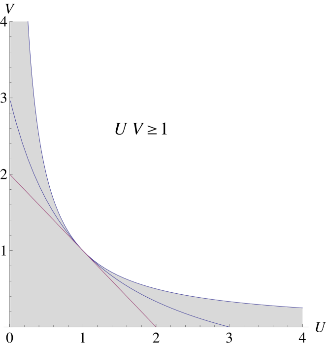
Figure 4: (Color online) The three separable conditions for the Gaussian states are described by the three curves on the $U$-$V$ plane associated with the variances for the EPR-like operators $(U,V)$. The three curves are inscribed at the single point $(U,V)=(1,1)$. The product condition of Eq. (8) implies that any state is entangled if its location on the $U$-$V$ plane $(U,V)$ is below the inverse proportional curve $UV=1$ (gray regime). The boundary of the sum condition of Eq. (11) is given by the straight line $U+V=2$. The boundary of the overlap condition of Eq. (26) for the Gaussian states in the standard form is given by $(U+1)(V+1)=4$, which includes the three points $(1,1)$, $(3,0)$, and $(0,3)$. This curve is lying in the middle of the two lines. It shows that the performance of the overlap condition is in between the product condition and the sum condition.

VI Experimental measurement schemes

In this section we describe how to estimate the state-overlap to the EPR-like correlated classical mixture $\langle\Gamma G_{\lambda}^{\prime}\rangle$ of Eq. (27) in experiments.

The heterodyne measurement corresponds to a projection to coherent states and its positive-operator-valued-measure elements are symbolically written as $\{|\alpha\rangle\langle\alpha|/\pi\}$. If we perform heterodyne measurement each of the two modes $A$ and $B$, then we can obtain the joint probability distribution associated with the projection to the product of the coherent states $\left|\alpha\right\rangle_{A}\left|\beta\right\rangle_{B}$ where $\alpha$ and $\beta$ correspond to the outcomes of the measurement on the system $A$ and the system $B$, respectively. From this joint probability distribution, the strength of the coherent-state-based EPR-like correlation $\langle\Gamma\hat{G}_{\lambda}^{\prime}\rangle$ for any pair of the parameters $(u,v)$ can be calculated. This enables us to check the overlap separable condition of Eq. (26) in principle. This may not be an efficient way for entanglement detection because the heterodyne statistics include the information of the full-tomographic reconstruction Leonhardt .

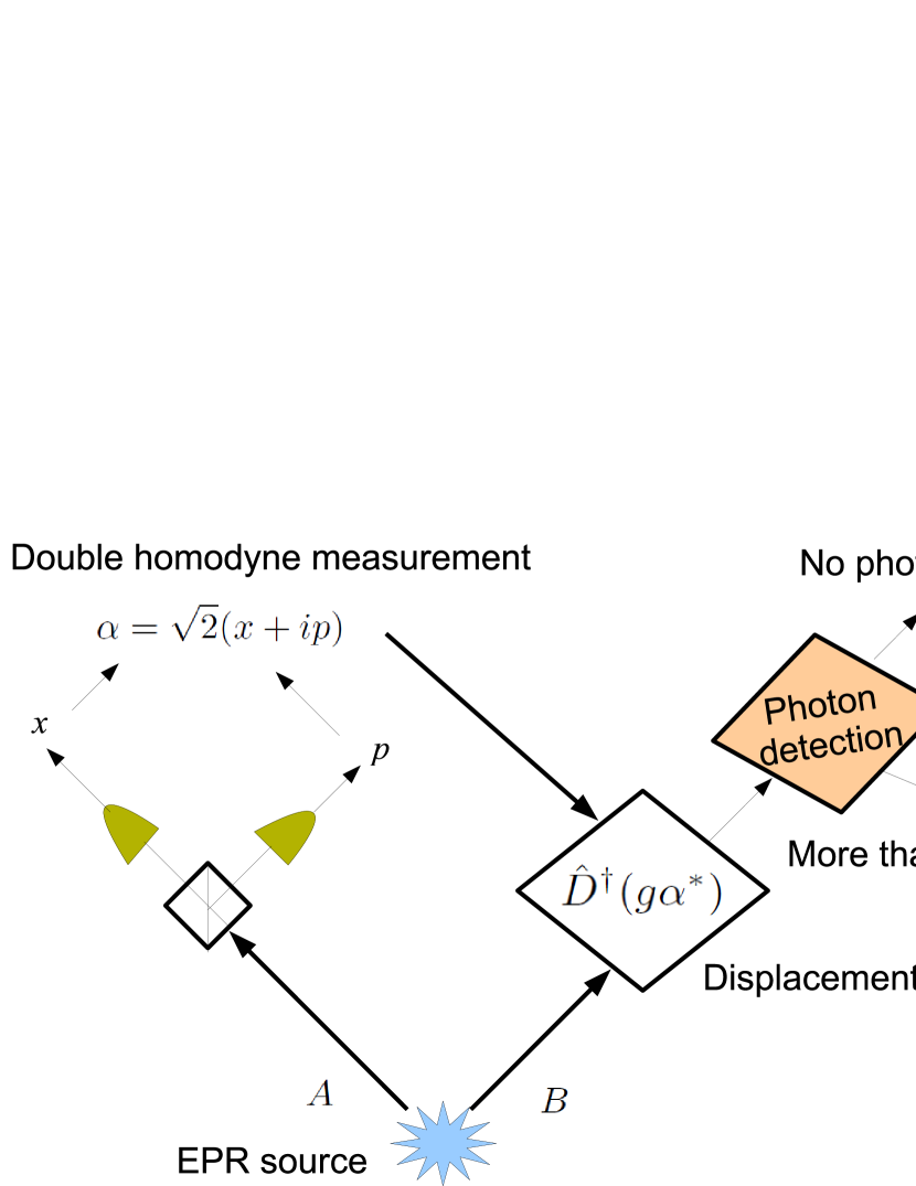
Figure 5: (Color online) The projection probability to a pair of coherent states $\left|\alpha\right\rangle\left|g\alpha^{*}\right\rangle$ can be measured by a heterodyne (double homodyne) measurement and a photon detection. The measurement outcome of the heterodyne measurement $(x,p)$ determines the amplitude of the coherent state $\alpha=\sqrt{2}(x+ip)$ of the mode $A$. The photon detection determines whether the number of the photon in the measured mode is zero or more than 1; It is the projection to one of the two subspaces $|0\rangle\langle 0|$ and $I-|0\rangle\langle 0|$ where $I=\sum_{n=0}^{\infty}|n\rangle\langle n|$. The photon detection of the mode $B$ after the displacement operation $\hat{D}^{\dagger}(g\alpha^{*})$ gives the information whether or not the state is initially in the coherent state $\left|g\alpha^{*}\right\rangle=\hat{D}(g\alpha^{*})\left|0\right\rangle$ because this state becomes vacuum after the displacement as $\hat{D}^{\dagger}(g\alpha^{*})\left|g\alpha^{*}\right\rangle=\left|0\right\rangle$.

In turn, if a pair of the parameters $(u,v)$ is specified beforehand, we only need to consider the probability associated with the specific pairs of the states $\left|\alpha\right\rangle_{A}\left|g\alpha^{*}\right\rangle_{B}$ with $g=v/u$. In order to measure this probability, a possible measurement process is composed of a heterodyne measurement and a photon detection with a feedforward control as in FIG. 5. We first perform the heterodyne measurement on the system $A$. Then, according to the outcome of the heterodyne measurement $\alpha$, we apply the displacement operation with an amount of the displacement $g\alpha^{*}$ on the system $B$. Finally, we perform the photon detection of the system $B$. It confirms whether or not the system $B$ was $\left|g\alpha^{*}\right\rangle$. This is because the displacement $\hat{D}^{\dagger}(g\alpha^{*})$ transforms the coherent state $\left|g\alpha^{*}\right\rangle$ to the vacuum state as $\left|0\right\rangle=\hat{D}^{\dagger}(g\alpha^{*})\left|g\alpha^{*}\right\rangle$ and the vacuum state is correctly discriminated by the photon detection as the no-photon event. This measurement technique has been demonstrated recently Wittmann08 ; Tsujino10 ; Tsujino11 . Repeating this process we can obtain the probability that the pair state $\left|\alpha\right\rangle_{A}\left|g\alpha^{*}\right\rangle_{B}$ is contained in the total system initially. From the measured expectation values $\langle|\alpha\rangle\langle\alpha|\otimes|g\alpha^{*}\rangle\langle g\alpha^{*}|\rangle$, a class of the separable conditions associated with Eq. (31) can be checked as well.

VII Conclusion

We have introduced the notion of the coherent-state-based EPR-like correlation as a state-overlap to a classically correlated coherent-state mixture. We have shown that the separable condition with this state-overlap is capable of detecting entanglement of two-mode Gaussian states. The separable threshold was derived by using the partial transposition on a limitation of the phase-space localization. A parallel formulation was given for the product separable condition concerning the standard EPR-like correlation. We have also addressed how to detect the state-overlap experimentally by the heterodyne detection and the following photon detection with a feedforward control.

This work was supported by GCOE Program “The Next Generation of Physics, Spun from Universality and Emergence” from MEXT of Japan. R.N. acknowledges support from JSPS.

References

• (1) A. Einstein, B. Podolsky, and N. Rosen, Phys. Rev. 47, 777 (1935).
• (2) M.D. Reid, P.D. Drummond, W.P. Bowen, E.G. Cavalcanti, P.K. Lam, H.A. Bachor, U.L. Andersen, and G. Leuchs, Rev. Mod. Phys. 81, 1727, (2009).
• (3) R. Horodecki, P. Horodecki, M. Horodecki, and K. Horodecki, Rev. Mod. Phys. 81, 865 (2009).
• (4) G. Adesso and F. Illuminati, J. Phys. A 40, 7821 (2007).
• (5) O. GΓΌhne and G. TΓ³th, Phys. Rep. 474, 1 (2009).
• (6) L-M. Duan, G. Giedke, J.I. Cirac, and P. Zoller, Phys. Rev. Lett. 84 2722 (2000).
• (7) A. Peres, Phys. Rev. Lett. 77, 1413 (1996).
• (8) R. Simon, Phys. Rev. Lett. 84, 2726 (2000).
• (9) G. Giedke, L. Duan, J.I. Cirac, and P. Zoller, Quant. Info. Comp. 1, 79 (2001).
• (10) E. Shchukin and W. Vogel, Phys. Rev. Lett. 95, 230502 (2005).
• (11) A. Miranowicz, M. Piani, P. Horodecki, and R. Horodecki, Phys. Rev. A 80, 052303 (2009).
• (12) S. L. Braunstein, and P. van Loock, Rev.Β Mod.Β Phys.Β 77, 513 (2005); N.J. Cerf, G. Leuchs, and E.S. Polzik (eds), Quantum Information with Continuous Variables of Atoms and Light, (Imperial College Press, London, 2007); U.L. Andersen, G. Leuchs, and C. Silberhorn, Laser&Photon. Rev. 1 (2009); K. Hammerer, A.S. Sorensen, and E.S. Polzik, Rev. Mod. Phys. 82, 1041 (2010).
• (13) F. Grosshans, N. J. Cerf, J. Wenger, R. Tualle-Brouri, Ph. Grangier, Quantum Inf. Comput. 3, 535 (2003); C. Weedbrook, A. M. Lance, W. P. Bowen, T. Symul, T. C. Ralph, and P. K. Lam, Phys. Rev. Lett. 93, 170504 (2004); S. Lorenz, J. Rigas, M. Heid, U. L. Andersen, N. LΓΌtkenhaus, and G. Leuchs Phys. Rev. A 74, 042326 (2006); J. Rigas, O. GΓΌhne, and N. LΓΌtkenhaus, Phys. Rev. A 73, 012341 (2006).
• (14) K. Banaszek and K. WΓ³dkiewicz, Phys. Rev. Lett. 82, 2009 (1999).
• (15) P. Marek, M.S. Kim, and J. Lee, Phys. Rev. A 79, 052315 (2009).
• (16) A. Miranowicz, M. Bartkowiak, X. Wang, Y.-x. Liu, and F. Nori, Phys. Rev. A 82, 013824 (2010).
• (17) R. Namiki, Phys. Rev. A83, 042323 (2011).
• (18) S. L. Braunstein, C.A. Fuchs, and J. Kimble, J. Mod. Opt 47, 267 (2000).
• (19) K. Hammerer, M.M. Wolf, E.S. Polzik, and J.I. Cirac, Phys. Rev. Lett. 94, 150503 (2005).
• (20) R. Namiki, Phys. Rev. A 78, 032333 (2008).
• (21) T. Takano, M. Fuyama, R. Namiki, and Y. Takahashi, Phys. Rev. A 78, 010307(R) (2008).
• (22) R. Namiki, S.-I.-R. Tanaka, T. Takano, and Y. Takahashi, Appl. Phys. B 105, 197-201 (2011).
• (23) R. Namiki, M. Koashi, and N. Imoto, Phys. Rev. Lett.101, 100502 (2008).
• (24) H. HΓ€seler, T. Moroder, and N. LΓΌtkenhaus, Phys. Rev. A 77, 032303 (2008).
• (25) M. Owari, M.B. Plenio, E.S. Polzik, A. Serafini, and M.M. Wolf, New J. Phys. 10, 113014 (2008).
• (26) G. Adesso and G. Chiribella, Phys. Rev. Lett. 100, 170503 (2008).
• (27) J. Calsamiglia, M. Aspachs, R. Munoz-Tapia, and E. Bagan, Phys. Rev. A 79, 050301 (2009).
• (28) H. HΓ€seler and N. LΓΌtkenhaus, Phys. Rev. A 80, 042304 (2009).
• (29) M. Guta, P. Bowles, and G. Adesso, Phys. Rev. A 82, 042310 (2010).
• (30) H. HΓ€seler and N. LΓΌtkenhaus, Phys. Rev. A 81, 060306(R) (2010).
• (31) N. Killoran, H. HΓ€seler, and N. LΓΌtkenhaus, Phys. Rev. A 82, 052331 (2010).
• (32) N. Killoran and N. LΓΌtkenhaus, Phys. Rev. A 83, 052320 (2011).
• (33) R. Namiki and Y. Tokunaga, Phys. Rev. A 85, 010305(R) (2012).
• (34) G.S. Agarwal and A. Biswas, New. J. Phys. 7, 211, (2005).
• (35) M.D. Reid, Phys. Rev. A 40, 913 (1989).
• (36) S.M. Tan, Phys. Rev. A 60, 2752 (1999).
• (37) S. Mancini, V. Giovannetti, D. Vitali, and P. Tombesi, Phys. Rev. Lett. 88, 120401 (2002).
• (38) V. Giovannetti, S. Mancini, D. Vitali, and P. Tombesi, Phys. Rev. A 67, 022320 (2003).
• (39) P. Hyllus and J. Eisert, New J. Phys. 8, 51 (2006).
• (40) K. Fujikawa, Phys. Rev. A 79, 032334 (2009); Phys. Rev. A 80, 012315 (2009).
• (41) R. Namiki, J. Phys. Soc. Jpn., 79, 013001 (2010).
• (42) R. Namiki, Phys. Rev. A83, 040302(R) (2011).
• (43) The symplectic eigenvalues are obtained when set we set $\kappa=v/u$, s=Ξ»/u2π‘ πœ†superscript𝑒2s=\lambda/u^{2} on the expression of $\nu_{\pm}$ in Ref. namiki11R .
• (44) U. Leonhardt, Measuring the Quantum State of Light (Cambridge, 1997).
• (45) C. Wittmann, M. Takeoka, K. N. Cassemiro, M. Sasaki, G. Leuchs, and U. L. Andersen, Phys. Rev. Lett. 101, 210501 (2008).
• (46) K. Tsujino, D. Fukuda, G. Fujii, S. Inoue, M. Fujiwara, M. Takeoka, and M. Sasaki, Opt. Express 18, 8107 (2010).
• (47) K. Tsujino, D. Fukuda, G. Fujii, S. Inoue, M. Fujiwara, M. Takeoka, and M. Sasaki, Phys. Rev. Lett. 106, 250503 (2011).