Fully Retroactive Approximate Range
and Nearest Neighbor Searching

Abstract

We describe fully retroactive dynamic data structures for approximate range reporting and approximate nearest neighbor reporting. We show how to maintain, for any positive constant $d$, a set of $n$ points in $\mathbb{R}^{d}$ indexed by time such that we can perform insertions or deletions at any point in the timeline in $O(\log n)$ amortized time. We support, for any small constant $\epsilon>0$, $(1+\epsilon)$-approximate range reporting queries at any point in the timeline in $O(\log n+k)$ time, where $k$ is the output size. We also show how to answer $(1+\epsilon)$-approximate nearest neighbor queries for any point in the past or present in $O(\log n)$ time.

1 Introduction

Spatiotemporal data types are intended to represent objects that have geometric characteristics that change over time (e.g., see [34, 28, 1]).

The important feature of such objects is that their critical characteristics, such as when they appear and disappear in a data set, exist in a timeline. The representation of such objects has a number of important applications, for instance, in video and audio processing, geographic information systems, and historical archiving. Moreover, due to data editing or cleaning needs, spatiotemporal data sets may need to be updated in a dynamic fashion, with changes that are made with respect to the timeline. Some possible examples of such dynamic updates include:

• A video editor may wish to add a 3-second video segment at the 20-second mark in a 27-second video and have the result be a seamless 30-second video (say, for a television commercial).

• A credit reporting company might need to remove some historical transactions in a consumer’s credit report to reflect the fact that these transactions were entered in error.

• Some of the historical trajectories in a collection of GPS traces may need to be changed to correct calibration errors that are discovered only after subsequent post-processing.

Thus, in this paper we are interested in methods for dynamically maintaining geometric objects that exist in the context of a timeline. Queries and updates happen in real time, but are indexed in terms of the timeline. For instance, one can ask to mark an object to exist for the first time at time index $t_{0}$, that is, to be inserted at time $t_{0}$. Likewise, one may ask to mark an object so it is identified as removed as of time index $t_{1}$, that is, to be deleted at time $t_{1}$. One may also ask to query the data set as of time index $t_{2}$, say, to ask for an approximate nearest neighbor of a point $p$ as of time index $t_{2}$. These updates and queries occur in real time with the intent that the timeline for the data set is made immediately consistent after each update and each query is performed correctly with respect to the current state of the timeline.

For example, suppose we have a set of 1-dimensional points, $X=\{1,4,7,10,13\}$, so that each $x\in X$ is inserted into the timeline at time index $t=x$ and never removed. If we then do a nearest-neighbor query for $6$ at time index $12$, the result would be $7$. But if we then revise the timeline so that $6$ is inserted at time index $6$, and we repeat the above nearest-neighbor query, then the answer would be $6$. Thus, our intent is that each update we make to the data set should propagate through the timeline in a consistent fashion, so that future queries made with respect to the timeline are answered correctly. Of course, we cannot go back in real time to change the answers to queries done in the (real) past with respect to the state of the timeline when that query was made.

In this paper, we are specifically interested in the dynamic maintenance of a set of $d$-dimensional points that appear and disappear from a data set in terms of indices in a timeline, for a given fixed constant $d\geq 1$. Points should be allowed to have their appearance and disappearance times changed, with such changes reflected forward in the timeline. We also wish to support time-indexed approximate range reporting and nearest-neighbor queries in such data sets. That is, we are interested in the dynamic maintenance of spatiotemporal point sets with respect to these types of geometric queries.

1.1 Related Work

Approximate Searching.

Arya and Mount [6] introduce the approximate nearest neighbor problem for a set of points, $S$, such that given a query point $q$, a point of $S$ will be reported whose distance from $q$ is at most a factor of $(1+\epsilon)$ from that of the true nearest neighbor of $q$. Arya et al. [8] show that such queries can be answered in $O(\log n)$ time for a fixed constant $\epsilon>0$. Chan [14] shows how to achieve a similar bound. Arya and Mount [7] also introduce the approximate range searching problem for a set, $S$, where a axis-parallel rectangle $R$ is given as input and every point in $S$ that is inside $R$ by a distance of at least $\epsilon$ is reported as output and no point of $S$ outside $R$ is reported. Let $k$ be the number of points reported. Arya and Mount show that such queries can be answered in $O(\log n+k)$ time for fixed constant $\epsilon>0$. Eppstein et al. [26] describe the skip quadtree structure, which supports $O(\log n+k)$-time approximate range searching as well as $O(\log n)$-time point insertion and deletion.

Our approach to solving approximate range searching and approximate nearest neighbor problems are based on the quadtree structure [42]. In this structure, regions are defined by squares in the plane, which are subdivided into four equal-sized squares for any regions containing more than a single point. So each internal node in the underlying tree has up to four children and regions have optimal aspect ratios. Typically, this structure is organized in a compressed fashion [4, 11, 12, 19], so that paths in the tree consisting of nodes with only one non-empty child are compressed to single edges. This structure is related to the balanced box decomposition (BBD) trees of Arya et al. [6, 7, 8], where regions are defined by hypercubes with smaller hypercubes subtracted away, so that the height of the decomposition tree is $O(\log n)$. Similarly, Duncan et al. [25] define the balanced aspect-ratio (BAR) trees, where regions are associated with convex polytopes of bounded aspect ratio, so that the height of the decomposition tree is $O(\log n)$.

Computational Geometry with respect to a Timeline.

Although we are not familiar with any previous work on retroactive $d$-dimensional approximate range searching and nearest-neighbor searching, we nevertheless would like to call attention to the fact that incorporating a time dimension to geometric constructions and data structures is well-studied in the computational geometry literature.

• Atallah [9] studies several dynamic computational geometry problems, including convex hull maintenance, for points moving according to fixed trajectories, showing an important connection between such problems and Davenport-Schinzel sequences. This work has been followed by a large body of subsequent work on additional connections between geometry, moving objects, and Davenport-Schinzel sequences. (E.g., see [48].)

• Subsequently, a number of researchers have studied geometric motion problems in the context of kinetic data structures (e.g., see [3, 10, 33, 32]). In this framework, a collection of geometric objects is moving according to a fixed set of known trajectories, and changes can only happen in the present. The goal is to maintain a data structure that supports geometric queries on this set with respect to the “current” time. As time progresses, the data structure needs to be updated, either because internal conditions about its state are triggered or because an object changes its trajectory.

• Sarnak and Tarjan [47] and Driscoll et al. [24] introduce the concept of persistent data structures, which support time-related operations where updates occur in the present and queries can be performed in the past, but updates in the past fork off new timelines rather than propogate changes forward in the same timeline. Such structures have been used in a number of applications, such as in planar point location, which use space-sweeping operations to construct data structures based on a static-to-dynamic-to-static framework.

All of this previous work differs from the approach we are taking in this paper, since in these previous approaches objects are not expected to be retroactively changed “in the past.”

Demaine et al. [20] introduce the concept of retroactive data structures, which is the framework we follow in this paper. In this approach, a set of data is maintained with respect to a timeline. Insertions and deletions are defined with respect to this timeline, so that each insertion has a time parameter, $t$, and so does each deletion. Likewise, queries are performed with respect to the time parameter as well. The difference between this framework and the dynamic computational geometry approaches mentioned above, however, is that updates can be done retroactively “in the past,” with the changes necessarily being propagated forward. If queries are only allowed in the current state (i.e., with the highest current time parameter), then the data structure is said to be partially retroactive. If queries can be done at any point in the timeline, then the structure is said to be fully retroactive. Demaine et al. [20] describe a number of results in this framework, including a fully-retroactive 1-dimensional structure for successor queries with $O(\log^{2}n)$-time performance. They also show that any data structure for a decomposable search problem can be converted into a fully retroactive structure at a cost of increasing its space and time by a logarithmic factor.

Acar et al. [2] introduce an alternate model of retroactivity, which they call non-oblivious retroactivity. In this model, one maintains the historical sequence of queries as well as insertions and deletions. When an update is made in the past, the change is not necessarily propagated all the way forward to the present. Instead, a non-oblivious data structure returns the first operation in the timeline that has become inconsistent, that is an operation whose return value has changed because of the retroactive update. As mentioned above, we only consider the original model of retroactivity as defined by Demaine et al. [20] in this paper.

Blelloch [13] and Giora and Kaplan [31] consider the problem of maintaining a fully retroactive dictionary that supports successor or predecessor queries. They both base their data structures on a structure by Mortensen [39], which answers fully retroactive one dimensional range reporting queries, although Mortensen framed the problem in terms of two dimensional orthogonal line segment intersection reporting. In this application, the $x$-axis is viewed as a timeline for a retroactive data structure for 1-dimensional points. The insertion of a segment $[(x_{1},y),(x_{2},y)]$ corresponds to the addition of an insert of $y$ at time $x_{1}$ and a deletion of $y$ at time $x_{2}$. Likewise, the removal of such a segment corresponds to the removal of these two operations from the timeline. For this 1-dimensional retroactive data structuring problem, Blelloch and Giora and Kaplan give data structures that support queries and updates in $O(\log n)$ time. Dickerson et al. [22] describe a retroactive data structure for maintaining the lower envelope of a set of parabolic arcs and give an application of this structure to the problem of cloning a Voronoi diagram from a server that answers nearest-neighbor queries.

1.2 Our Results

In this paper, we describe fully retroactive dynamic data structures for approximate range reporting and approximate nearest neighbor searching. We show how to maintain, for any positive constant, $d\geq 1$, a set of $n$ points in $\mathbb{R}^{d}$ indexed by time such that we can perform insertions or deletions at any point in the timeline in $O(\log n)$ amortized time. We support, for any small constant $\epsilon>0$, $(1+\epsilon)$-approximate range reporting queries at any point in the timeline in $O(\log n+k)$ time, where $k$ is the output size. Note that in this paper we consider circular ranges defined by a query point $q$ and radius $r$. We also show how to answer $(1+\epsilon)$-approximate nearest neighbor queries for any point in the past or present in $O(\log n)$ time. Our model of computation is the real RAM, as is common in computational geometry algorithms (e.g., see [44]).

The main technique that allows us to achieve these results is a novel, multidimensional version of fractional cascading, which may be of independent interest. Recall that in the (1-dimensional) fractional cascading paradigm of Chazelle and Guibas [17, 18], one searches a collection of sorted lists (of what are essentially numbers), which are called catalogs, that are stored along nodes in a search path of a catalog graph, $G$, for the same element, $x$. In multidimensional fractional cascading, one instead searches a collection of finite subsets of $\mathbb{R}^{d}$ for the same point, $p$, along nodes in a search path of a catalog graph, $G$. In our case, rather than have each catalog represented as a one-dimensional sorted list, we instead represent each catalog as a multidimensional “sorted list,” with points ordered as they would be visited in a space-filling curve (which is strongly related to how the points would be organized in a quadtree, e.g., see [46, 12]).

By then sampling in a fashion inspired by one-dimensional fractional cascading, we show how to efficiently perform repeated searching of multidimensional catalogs stored at the nodes of a search path in a suitable catalog graph, such as a segment tree (e.g., see [44]), with each of the searches involving the same $d$-dimensional point or region.

Although it is well known that space-filling curves can be applied to the problem of approximate nearest neighbor searching, we are not aware of any extension of space-filling curves to approximate range reporting. Furthermore, we believe that we are the first to leverage space-filling curves in order to extend dynamic fractional cascading into a multi-dimensional problem.

2 A General Approach to Retroactivity

Recall that a query $Q$ is decomposable if there is a binary operator $\square$ (computable in constant time) such that $Q(A\cup B)=\square(Q(A),Q(B))$. Demaine et al. [20] showed that we can make any decomposable search problem retroactive by maintaining each element ever inserted in the structure as a line segment along a time dimension between the element’s insertion and deletion times. Thus each point $p$ in $R^{d}$ is now represented by a line segment parallel to the time-axis in $R^{d+1}$ dimensions. For example when extending the query to be fully-retroactive, a one-dimensional successor query becomes a two-dimensional vertical ray shooting query, and a one-dimensional range reporting query becomes a two-dimensional orthogonal segment intersection query (Figure 1).

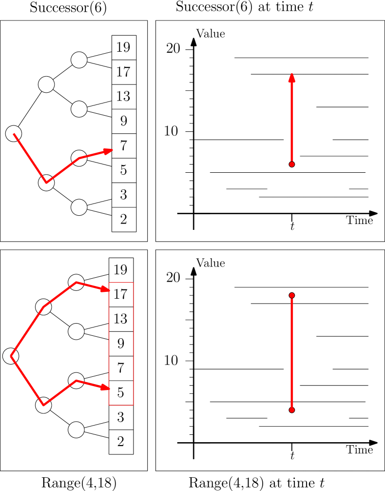
Figure 1: Examples of how a $d$ dimensional query on points becomes a $d+1$ dimensional query on segments. Here we illustrate how a one-dimensional successor query becomes a two dimensional vertical ray shooting query, and a one-dimensional range reporting query becomes a two-dimensional segment intersection query.

Thus, we maintain a segment tree to allow searching over the segments in the time dimension, and augment each node of the segment tree with a secondary structure supporting our original query in $d$ dimensions. Let $S$ be the set of nodes in the segment tree on a root-to-leaf path searching down for $t$ in the time dimension. To answer a fully-retroactive query, we perform the same $d$-dimensional query at each node in $S$. This transformation costs an extra $\log n$ factor in space, query time, and update time, which we would nevertheless like to avoid.

Recall that Mortensen [39] and Giora and Kaplan [31] both solve the fully-retroactive versions of decomposable search problems, and are both able to avoid the extra $\log n$ factor in query and update time. Therefore inspired by their techniques, we propose the following as a general strategy for optimally solving the fully-retroactive version of any decomposable search problem.

1. Suppose we have an optimal data structure $D$ for the non-retroactive problem which supports queries in polylogarithmic time $T(n)$.

2. Represent each $d$-dimensional point as a line segment in $d+1$ dimensions.

3. Build a weight-balanced segment tree with polylogarithmic branching factor over the segments as described by [31].

4. Augment the root of the segment tree with an optimal search structure $D$.

5. Augment each node of the segment tree with a colored dynamic fractional cascading (CDFC) data structure.

6. Perform a retroactive query at time $t$ by performing the non-retroactive query on the non-retroactive data structure at the root of the segment tree, and for each node on the search path for $t$ in the segment tree, perform the query in each of the CDFC structures (Figure 2).

The CDFC data structure must be cleverly tuned to support a colored (but non-retroactive) version of the $d$-dimensional query in $O(T(n)\cdot\log\log n/\log n)$ time. In a colored query, each element in the structure is given a color, and the query also specifies a set of colors. We only return elements whose color is contained in the query set. The colors are required because the segment tree has high degree. Each color represents a pair of children of the current node in the segment tree. Thus we encode which segments overlap the search path via their colors. Since the segment tree has a polylogarithmic branching factor, we spend $T(n)$ time searching at the root and $O(T(n)\cdot\log\log n/\log n)$ time searching in the CDFC structures at each of the $O(\log\log n/\log n)$ nodes. Therefore, the total time required by a query is an optimal $O(T(n))$. Updates follow a similar strategy, but may require us to periodically rebuild sections of the segment tree. We can still achieve the desired (amortized) update time, and the analysis closely follows [31].

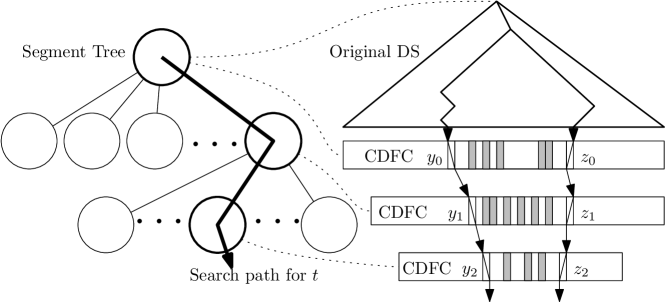
Figure 2: An application of our strategy to a fully-retroactive one-dimensional range reporting query. Shaded elements represent elements with colors indicating they are present at time $t$.

One of the key difficulties in applying this strategy lies in the design of the colored dynamic fractional cascading data structure, especially in problems where the dimension $d>1$. In fact, the authors are not aware of any previous application of dynamic fractional cascading techniques to any multidimensional search problem. However, in the following we show how techniques using space filling curves can be applied to extend the savings of fractional cascading into a multidimensional domain. First, we apply the above strategy in the simpler case when $d=1$. Then we extend this result using space filling curves to support Fully-Retroactive range reporting queries and approximate nearest neighbor queries in $\mathbb{R}^{d}$. Note that in one dimension a nearest neighbor query reduces to a successor and predecessor query.

Lemma 2.1.

There exists a colored dynamic fractional cascading data structure which supports updates in $O(\log\log N)$ amortized time, colored successor and predecessor queries in $O(\log\log N)$ worst case time and colored range reporting queries in $O(\log\log N+k)$ worst case time, where $N$ is the number of elements stored and $k$ is the number of elements reported.

Proof.

We extend the generalized union-split-find structure of [31] to also support colored range queries. See Appendix B. ∎

Space Filling Curves.

The z-order, due to Morton [40], is commonly used to map multidimensional points down to one dimension. By now space filling curves are well-studied and multiple authors have applied them specifically to quadtrees (e.g., see [46, 12]) and approximate nearest neighbor queries [21, 16, 14, 37]. However, we extend their application to approximate range searching as well. Furthermore, we believe that we are the first to leverage space-filling curves to extend dynamic fractional cascading techniques to multidimensional problems such as these.

Lemma 2.2.

The set of points in any quadtree cell rooted at $[0,1)^{d}$ form a contiguous interval in the z-order.

Proof.

Due to Bern et al. [12]. See Appendix D for details. ∎

Lemma 2.3.

Let $P$ be a set of points in $\mathbb{R}^{d}$. Define a constant $c=\sqrt{d}(4d+4)+1$. Suppose that we have $d+1$ lists $P+v^{j},j=0,\ldots,d$, each one sorted according to its z-order. We can find a query point $q$’s $c$-approximate nearest neighbor in $P$ by examining the the $2(d+1)$ predecessors and successors of $q$ in the lists.

Proof.

See Appendix D. ∎

3 Main Results

In this section we give our primary results: data structures for fully-retroactive approximate range queries and fully-retroactive approximate nearest neighbor (ANN) queries. Recall that an approximate range query $report(q,r,\epsilon,t)$ defines an inner range $Q^{-}$, the region within a radius $r$ of the query point $q$ and an outer range $Q^{+}$, the area within a radius of $(1+\epsilon)r$ of $q$. We want to return all the points inside $Q^{-}$ and exclude all points outside $Q^{+}$ for a particular point in time $t$. Points that fall between $Q^{-}$ and $Q^{+}$ at time $t$ may or may not be reported. Points not present at time $t$ will never be reported.

Theorem 3.1 (Fully-Retroactive Approximate Range Queries).

For any positive constant $d\geq 1$, we can maintain a set of $n$ points in $\mathbb{R}^{d}$ indexed by time such that we can perform insertions or deletions at any point in the timeline in $O(\log n)$ amortized time. We support for any small constant $\epsilon>0$, $(1+\epsilon)$-approximate range reporting queries at any point in the timeline in $O(\log n+k)$ time, where $k$ is the output size. The space required by our data structure is $O(n\log n/\log\log n)$.

Proof.

We follow the general strategy outlined in Section 2. We augment the root of the segment tree with a skip-quadtree, an optimal structure for approximate range and nearest neighbor queries in $\mathbb{R}^{d}$. We also augment each node of the segment tree with a specialized CDFC structure which we now describe.

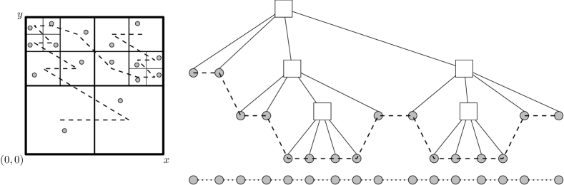
Figure 4: The z-order curve corresponds to the order the leaves would be visited in an in-order traversal of the quadtree. We can store the points in a linked list in this order. Any element between two elements $i,j$ in the linked list must fall in the same quadtree cell as $i$ and $j$.

We extend the CDFC structure from Lemma 2.1 to maintain $d$-dimensional points such that given a query set of colors $C_{q}$ and $d$-dimensional quadtree cell, it returns all points contained in that cell with colors in $C_{q}$. By Lemma 2.2, for all points $y,q,z$ such that $y<q<z$ in the z-order, any quadtree cell containing $y$ and $z$ must also contain $q$. Furthermore, for a given quadtree, each cell is uniquely defined by the leftmost and rightmost leaves in the cell’s subtree. Therefore, the $d$-dimensional cell query reduces to a one-dimensional range query in the z-order on the unique points which define the quadtree cell (Figure 4). Thus, by leveraging Lemma 2.1 and maintaining the points according to their z-order, we support the required query in $O(\log\log n+k)$ time.

The skip-quadtree tree contains all the points ever inserted into our data structure, irrespective of the time that they were inserted or deleted. The inner and outer range of a query partition the set of quadtree cells into the three subsets: the inner cells, which are completely contained in $Q^{+}$, the outer cells, which are completely disjoint from $Q^{-}$, and the stabbing cells, which partially overlap $Q^{+}$ and $Q^{-}$. Eppstein et al. [27] showed that a skip-quadtree can perform an approximate range query in $O(\log n+\epsilon^{1-d})$ time expected and with high probability, or worst case time for a deterministic skip-quadtree. Using their algorithm we can find the set $I$ of $O(\epsilon^{1-d})$ disjoint inner cells in the same time bound. Based on the correctness of their algorithm we know that the set of points we need to report are covered by these cells. We report the points present at time $t$ as follows: For each cell $i\in I$, if $i$ is a leaf, we report only the points in $i$, which are present at time $t$ in constant time. Otherwise, we find the first and last leaves $y_{0}$ and $z_{0}$ according to an in-order traversal of $i$’s subtree in $O(\log n)$ time. Then we perform a fully-retroactive range query on cell $i$ in the segment tree, using $z_{0}$ and $y_{0}$ to guide the query on cell $i$ in the CDFC structures. Correctness follows since a point satisfies the retroactive range query if and only if it is in one of the cells we examine and is present at time $t$.

For each of the $O(\epsilon^{1-d})$ cells in $I$ we spend $O(\log n+k_{i})$ time and so the total running time is $O(\epsilon^{1-d}\log n+k)=O(\log n+k)$, since $\epsilon$ is a small constant. The skip-quadtree is linear space, and thus the space usage is dominated by the segment tree. The total space required is $O(n\log n/\log\log n)$. ∎

Corollary 3.2 (Fully-Retroactive ANN Queries.).

We can maintain, for any positive constant, $d\geq 1$, a set of $n$ points in $\mathbb{R}^{d}$ indexed by time such that we can perform insertions or deletions at any point in the timeline in $O(\log n)$ amortized time. We support, for any small constant $\epsilon>0$, $(1+\epsilon)$-approximate nearest neighbor queries for any point in the past or present in $O(\log n)$ time. The space required by our data structure is $O(n\log n/\log\log n)$.

Proof.

By combining the data structure of [31] with Lemma 2.3 and storing the $d$-dimensional points in that structure according to their z-order, we already have a data structure for fully-retroactive $c$-approximate nearest neighbor queries. However, $c$ is polynomial function of $d$, and for $d=2$, $c$ is already greater than 15. In order to support $(1+\epsilon)$ nearest neighbor queries for any $\epsilon>0$, we require the data structure of the previous theorem.

We know from Lemma 2.3 that we can find a $c$-approximate nearest neighbor by using $d+1$ different shifts of the points. Therefore, we augment our data structure so that instead of a single CDFC structure at each segment tree node, we keep an array of $d+1$ CDFC structures corresponding to the z-order of each of the $d+1$ sets of shifted points. Given a point $q$, we can find a the predecessor and successor of $q$ at time $t$ in each of the $d+1$ z-orders in $O(d\log n)$ time. Out of these $2(d+1)$ points, let $p$ be the point that is closest to $q$. By Lemma 2.3, $p$ is a $c$-approximate nearest neighbor. Let $r$ be the distance between $p$ and $q$. As observed by multiple authors [5, 41, 35], we can find a $(1+\epsilon)$-approximate nearest neighbor via a bisecting search over the interval $[r/c,r]$. This search requires $O(\log(1/\epsilon))$ fully-retroactive spherical emptiness queries. We can support a retroactive spherical emptiness query in $O(\log n)$ time with only a slight modification to our retroactive approximate range query. Instead of returning $k$ points in the range, we just return the first point we find, or null if we find none. Thus the total time required is $O(d\log n+\log(1/\epsilon)\log n)=O(\log n)$ since we assume $\epsilon$ and $d$ are constant. The space usage only increases by a factor of $d$ when we store the $d+1$ shifted lists, and thus the space required is still $O(n\log n/\log\log n)$.

∎

Acknowledgments

This research was supported in part by the National Science Foundation under grants 0847968 and 0953071 and by the Office of Naval Research under (MURI) Award number N00014-08-1-1015.

Appendices

Appendix A Generalized Van Emde Boas (GVEB) Trees

Theorem A.1.

A GVEB structure with parameters $(N,M)$ uses $O(NC)$ space and can be initialized in $O(NC)$ worst case time, where $C=\log^{\frac{1}{4}}M$ is the number of colors supported. It requires a lookup table of size $O(M)$ and supports insert, delete and colored successor (find) queries in $O(\log\log N)$ worst case time. It also supports colored range reporting queries (report) in $O(\log\log N+k)$ time, where $k$ is the number of elements reported.

The Generalized van Emde Boas tree (GVEB) is an extension of the data structure by van Emde Boas et al. [49]. Recall that a van Emde Boas tree (VEB) is a recursive data structure that supports successor and predecessor queries for a fixed (monochrome) universe $U$ in $O(\log\log U)$ time. A recursive data structure is one that references itself over a smaller section of input as a part of its definition. For example, in a binary search tree, an internal node $v$ with key $k$ partitions the set of input keys into keys greater than $k$ that are stored recursively in the right subtree and keys less than $k$ that are stored recursively in the left subtree. Thus the children of each internal node are themselves binary search trees defined over a subset of the input.

To avoid tedious details, we make the typical assumption that $U$ is the set of integers in the range $[N]$ and that $N$ has the form $2^{2^{\ell}}$ for some positive integer $\ell$. Note that $\ell=O(\log\log N)$ is the number of levels of recursive structures. Each node of the VEB tree contains the following four fields: Min, Max, Bottom, and Top. The Min and Max fields contain the minimum and maximum elements in the node’s subtree. The VEB partitions $[N]$ into $\sqrt{N}$ buckets each of size $\sqrt{N}$. These buckets are stored in Top, a single recursive structure. Each bucket in Top points to a recursive VEB structure for a universe size of $\sqrt{N}$ in Bottom. The recursive structures in Bottom can be thought of as the children of the node, and the single structure in Top functions as an efficient way to search these children. If a key $k$ is the maximum or minimum integer in a particular recursive structure, then it is just stored in the Max or Min fields. Otherwise, it is stored recursively in Bottom$[k\textrm{ div }\sqrt{N}]$ as $k\mod\sqrt{N}$.

Let $N,M$ be two integers that fit in a machine word, and let $C=[\log^{\frac{1}{4}}M]$. The Generalized van Emde Boas (GVEB) data structure of [31] maintains a set of (key, color) pairs $(k,c)$ where $k$ is an integer in $[N]$ and $c$ is an integer in $C$. Let $C_{q}\subseteq C$ be a set of colors. The query find$(k_{q},C_{q})$ returns the successor of $k_{q}$ with color $c\in C_{q}$, i.e. we want to return the minimum key element $(k^{\prime},c^{\prime})$ such that $k^{\prime}\geq k_{q}$ and $c^{\prime}\in C_{q}$. GVEB supports find, insert and delete operations in $O(\log\log N)$ worst case time.

The GVEB tree is similar to the VEB tree, only instead of maintaining a single minimum and maximum integer in each recursive structure, we maintain a min and max for each color $c\in C$. Let $G$ be a GVEB structure. The Min and Max arrays are actually maintained via two arrays each (4 total) of size $|C|$: max-key, max-rank, min-key, min-rank. For each $c\in C$, max-key$[c]=\max\{k\ |(k,c)\in G\}$ and max-rank$[c]$ is the rank of max-key$[c]$. The arrays min-key and min-rank are defined symmetrically. Max and Min also each contain a q-heap, max-Q and min-Q, which contain all the elements in Max and Min respectively. Recall that the q-heap of [30] can store up to $\log^{\frac{1}{4}}M=|C|$ elements, requires a lookup table of size $M$, and supports successor and rank queries in constant time.

Finally, we precompute a table of size $O(M)$ that points to the maximum element in $G$ with a color in $C_{q}$ for every possible set $C_{q}$ and for each possible max-rank array. Together these data structures allow us to spend only constant time at each level of the structure during a find, insert, or delete operation, so that the time required for each operation is $O(\log\log n)$. For full details of how these operations work, see section 5.1 of [31].

In addition to the insert, delete, and find operations, we also require a one-dimensional colored range reporting query. Therefore we extend the GVEB $G$ to also support the query report$(i,j,C_{q})$, which returns the set of elements $\{(k,c)\in G|i\leq k\leq j,c\in C_{q}\}$. We also need an internal helper query reportany$(i,j,C_{q})$, which, for each color $c\in C_{q}$ such that the set $\{(k,c)|(k,c)\in G,i\leq k\leq j\}$ is non-empty, returns exactly one element from that set. For each color $c$ such that there exists an element $(k,c)\in G$, we maintain pointers to the successor and predecessor of $k$ with color $c$. We can maintain these pointers in $G$ with no additional asymptotic cost. Then to answer a report query, we first perform a reportany query, and then follow these pointers to find the rest of the elements in the range. We now describe how to perform the reportany query efficiently.

We will require the data structure from Lemma 3.2 of [39].

Lemma A.1.

We can maintain an array $A$ indexed by $C$ where each entry in $A$ is an integer in $[O(N)]$ such that updates to $A$ can be performed in constant time and such that given i and j we can calculate the set $\textrm{report}(A,i,j)=\{c\in C|i\leq A[c]\leq j\}$ in constant time. The space usage of $A$ is $O(|C|)$ and $A$ can be initialized in constant time.

Proof.

The structure uses a q-heap and a global lookup table of size $O(N)$ to maintain in a single word a table $B$ indexed by elements in $C$ such that $B[C]$ is the rank of $A[c]$ among the elements of $A$. See [39] for comparable details. This structure is similar to the max-rank data structure of the GVEB structure above, but instead of returning the rank of a single element, it returns the colors of the elements between two ranks as a single word. ∎

Let $min^{\prime}$ and $max^{\prime}$ each be data structures of the type in Lemma A.1. We add these structures to each recursive GVEB structure $G$ to answer the query reportany$(G,i,j,C_{q})$. The following algorithm follows how Mortensen answered the reportany query in his $S_{n}$ data structure [39], but differs in some important details. If $G=\emptyset$ or $i>j$, then there are no elements to report. Otherwise, we find elements to report from the min-key array as follows. Let $C_{r}=\texttt{report}(i,j,min^{\prime})$, and let $C_{min}=C_{q}\cap C_{r}$. We repeat this process to find elements in the max-key array. Let $C_{q}=C_{q}\backslash C_{r}$, the subset of query colors that we have not already reported, and let $C_{r}=\texttt{report}(i,j,max^{\prime})$, and $C_{max}=C_{q}\cap C_{r}$. We report the elements min-key$[c]$ for each $c\in C_{min}$ and max-key$[c]$ for each $c\in C_{max}$. Thus we have found all colors for which the minimum or maximum element of that color was in the range $[i,j]$, but there could be other colors for which there exists an element in the range $[i,j]$ but the minimum and maximum elements of that color were both outside the range. Therefore, we recursively search for elements with colors in $C_{q}=C_{q}\backslash(C_{min}\cup C_{max})$ via the following procedure. If $i=0$ or $j=N-1$, we return because there can be no additional elements to report–the max and min elements could not have both been outside the range. Otherwise, if $i\textrm{ div }\sqrt{N}=j\textrm{ div }\sqrt{N}$, then the range falls entirely inside a single bucket, and we can find the remaining elements with a single recursive call: reportany$(G.\texttt{Bottom}[i\textrm{ div }\sqrt{N}],i\mod\sqrt{N},j\mod\sqrt{N},C_{q})$. Otherwise, the range spans multiple buckets, and we require 3 recursive calls:

1. reportany$(G.\texttt{Bottom}[i\textrm{ div }\sqrt{N}],i\mod\sqrt{N},\sqrt{N}-1,C_{q})$,

2. reportany$(G.\texttt{Top},i\textrm{ div }\sqrt{N}+1,j\textrm{ div }\sqrt{N}-1,C_{q})$,

3. reportany$(G.\texttt{Bottom}[j\textrm{ div }\sqrt{N}],0,j\mod\sqrt{N},C_{q})$, passing the $C_{q}$ parameter by reference.

The first recursive call (1) covers the last part of the first bucket, and the third recursive call (3) covers the first part of the last bucket. In both (1) and (3), we encounter the stopping condition: $i=0$ or $j=N-1$, and so we only need to examine min-key, max-key, $min^{\prime}$ and $max^{\prime}$. It is only the second recursive call (2) that may require additional recursion. Note that some of the elements returned by (2) not be actual elements, but rather pointers to recursive structures. So, as a final step we iterate over all the elements returned, and while there exists an element of color $c$ that is actually a pointer to some recursive structure $T$, we replace it with $T.\texttt{min-key}[c]$.

We now analyze the additional time and space cost of supporting the report query. First we note that the data structure of Lemma A.1 requires no more space than the Min and Max data structures. Therefore, the asymptotic space usage of our augmented GVEB is the same as the original GVEB, which was shown by [31] to be $O(N\cdot|C|)$. Second, observe that the data structure of Lemma A.1 can be updated in constant time, and only needs to be updated when we are already making changes on a given level of recursion. Therefore updates take $O(\log\log N)$, no more time than in the original GVEB. Finally, we consider the time required to perform a report query.

The first observation is that whenever we perform more than one recursive call in the reportany query, only one call requires non-constant work. It’s possible that in the replacement step, $T.\texttt{min-key}[c]$ may point to another substructure $T^{\prime}$, and we may need to follow $O(\log\log N)$ pointers to finally reach a true element. However, the second observation is that for each substructure $T$ that we examine, there are at least two elements that fall in the range and which we will ultimately report. Therefore we can answer the report query in time $O(\log\log n+k)$.

Appendix B Generalized Union-Split-Find (GUSF)

The generalized Union-Split-Find (GUSF) structure is an extension of the dynamic Union-Split-Find (USF) data structure [23, 45]. The USF structure maintains a list $L$ of elements from an ordered set, some of which are marked. It supports the following operations:

• FindNext$(x)$ returns the smallest element $x^{\prime}\geq x$ such that $x^{\prime}$ is marked.

• Add$(x,y)$ inserts a new unmarked element $x$ just before the element $y$.

• Remove$(x)$ removes an unmarked element $x$ from the list.

• Unmark$(x)$ (Union) changes $x$ from a marked element to an unmarked element.

• Mark$(x)$ (Split) changes $x$ from an unmarked element to a marked element.

The USF structure can be considered monochrome. Each element is either unmarked (white) or marked with a single color (black). The GUSF extends the USF to support a whole set of colors $C$ so that each element can either be unmarked, or marked with some subset of colors $C^{\prime}\subseteq C$. The query and update operations are extended accordingly. The GUSF also supports additional queries: a FindPrev query, which is symmetric to FindNext and a Report$(y_{1},y_{2},C_{q})$ query, which reports each element $y$ in the list such that $y_{1}\leq y\leq y_{2}$ once for each color in $C(y)\cap C_{q}$, where $C_{q}$ is a set of query colors and $C(y)$ is the set of colors with which element $y$ is marked.

Theorem B.1.

A GUSF data structure with parameter $N$ uses $O(N)$ space and supports updates in $O(\log\log N)$ amortized time, find queries in $O(\log\log N)$ worst case time and report queries in $O(\log\log N+k)$ worst case time. The find queries include FindNext$(x,C_{q})$ and FindPrev$(x,C_{q})$ query, which respectively find the successor and predecessor of $x$ with color $c\in C_{q}$. The query Report$(y_{1},y_{2},C_{q})$ reports each element $y$ such that $y_{1}\leq y\leq y_{2}$ once for each color in $C(y)\cap C_{q}$. Supported updates include Mark$(x,c)$, Unmark$(x,c)$, Add$(x)$ and Remove$(x)$.

Proof.

We employ a technique utilized in the Union-Split-Find data structure  [23, 45] and later adopted by [39] in his data structure for a colored linked list and [31] in their Generalized Union-Split-Find data structure. This technique simultaneously removes the requirement that the elements have integer keys and reduces the space required by our data structure. Let $L$ be our list and let $n=|L|\leq N$ be the number of elements in the list. The key idea is to group consecutive elements of the linked list into blocks of size $\Theta(\log^{\beta}n)$ for an appropriate small constant $\beta>3$. We label the blocks with integer labels such that the order of the labels indicates the order of the blocks in $L$. We maintain these labels using the order maintenance structure of Willard [50].

In each block $b$ we build a binary search tree $T_{b}$ and store the elements of $b$ in the leaves of $T_{b}$, ordered by their order in $L$. We augment the nodes of $T_{b}$ according to the techniques of [39] and [20]. Each element $y\in L$ is associated with a set of colors $C(y)$, where $|C(y)|=O(1)$. Thus, for each leaf $v_{y}$ in $T_{b}$ representing an element $y\in L$, we let $C(v_{y})=C(y)$. For each internal node $v$ in $T_{b}$ with children $u$ and $w$, we let $C(v)=C(u)\cup C(w)$. Hence we color each internal node with the union of the colors of its descendant leaves, and we color the root of $T_{b}$ with the union of the colors of all the elements in block $b$. We say a block has color $c$ if it contains a leaf with color $c$. Thus the colors of the block $b$ equal the colors of the root $r_{b}$. For each block we maintain a single array $b.\texttt{allleafs}$ of size $|b|=O(\log^{\beta}n)$ such that for each leaf $v_{y}\in b$, there is a pointer in $b.\texttt{allleafs}$ to $v_{y}$. We do not necessarily maintain the order of $b.\texttt{allleafs}$. to match the order of leaves in $b$, but we do maintain a list $b.\texttt{freelist}$ of unused indices in $b.\texttt{allleafs}$. We also keep an array $v.\texttt{leafs}$ indexed by $C$ in each internal node $v$ such that $v.\texttt{leafs}[c]\neq 0$ iff $v$ has a descendant leaf with color $c$, and $b.\texttt{allleafs}[v.\texttt{leafs}[c]]$ is a pointer to one such leaf. Each of the indices in $v.\texttt{leafs}$ is $O(\log\log n)$ bits and therefore the entire array $v.\texttt{leafs}$ can be stored in a single word. Furthermore, $C(v)$ can be determined in constant time by examining $v.\texttt{leafs}$. Lastly, for each leaf $v_{y}$, and color $c\in C(v_{y})$, we keep a pointer to predecessor and successor of $v_{y}$ with color $c$, thus creating a linked list over the leaves for each color $c\in C(r_{b})$.

We represent each block $b$ by the root $r_{b}$ of the tree $T_{b}$. We keep the roots in a linked list $B$. Since each block has size $\Theta(\log^{\beta}n)$, $|B|=O(n/\log^{\beta}n)$. We assign the roots integer labels according to their order using the order maintenance structure of Willard [50], denoted OM. We store the roots of the blocks in a GVEB structure (see Appendix A) $G$ with parameters $(N,M)$ according to their integer labels, where $N=\Theta(|B|)$. Given a root with integer label $k$ and colors $C(r_{b})$, we store one element $(k,c)$ in $G$ for each color $c\in C(r_{b})$. OM requires linear space. Insertions and deletions to OM can be performed in $O(\log^{2}|B|)$ worst case time, and may cause $O(\log^{2}|B|)$ integer labels to be updated.

• FindNext$(x,C_{q})$. This algorithm resembles that of [31]. However, instead of having a bit-vector $C(v)$ for each internal node $v$, $C(v)$ is represented implicitly by and calculated in constant time from the array $v.\texttt{leafs}$. We describe the algorithm here for completeness. If $C(x)\cap C_{q}\neq\emptyset$, then return $x$. Otherwise $x$ is contained in some block $b$, and therefore in a tree $T_{b}$. We traverse the path from $x$ to $r_{b}$, and look for the first node $y$ hanging to the right of this path such that $C_{q}\cap C(y)\neq\emptyset$. If such a node $y$ exists, then we find the leftmost leaf in $y$’s subtree with color $c\in C_{q}$ as follows. Let $v$ be a the current node we’re examining. If $v$ is a leaf, then return it. We repeat the following until we reach a leaf. Let $v_{\ell}$ and $v_{r}$ be the left and right children of $v$ respectively. If $C_{q}\cap C(v_{\ell})\neq\emptyset$, then set $v=v_{\ell}$. Otherwise set $v=v_{r}$. Clearly if a there exists a successor of $x$ in $T_{b}$ with color $c\in C_{q}$ we will find it. If not, then we find the block $b$’ with a color in $C_{q}$ with a query find query on $G$. If $b$’ exists then we repeat the above process to find the leftmost leaf with a color in $C_{q}$ in $T_{b}^{\prime}$. If not, then there is no successor of $x$ with color $c\in C_{q}$. It takes $O(\log\log n)$ time to perform the query in each block, and $O(\log\log N)=O(\log\log n)$ time to perform the query in $G$. Therefore the total time required is $O(\log\log n)$.

• FindPrev$(x,C_{q})$ finds the predecessor of $x$ with color $c\in C_{q}$ instead of the successor. It is supported symmetrically.

• Report$(y_{1},y_{2},C_{q})$. We handle the report query as described by [39]. This algorithm reports each element $y\in L$ such that $y_{1}\leq y\leq y_{2}$ once for each color in $C(y)\cap C_{q}$. Since the number of colors in $C(y)$ is constant, we can easily modify this procedure to only report each element once. Let $T_{1}$ be the tree for the block containing $y_{1}$ and let $T_{2}$ be the tree for the block containing $y_{2}$. We begin by searching bottom up in $T_{1}$ and $T_{2}$ to report elements to the right of $y_{1}$ in $T_{1}$ and to the left of $y_{2}$ in $T_{2}$ with colors in $C_{q}$. We can report these elements in $O(\log\log n+k)$ time using the allleafs array, leafs arrays, and the leaf lists. If $T_{1}\neq T_{2}$, then we also perform a report query in $G$ to find all the blocks between $T_{1}$ and $T_{2}$ with colors in $c\in C_{q}$. For each such block $b$ and color $c$ with root $r_{b}$, we can use leafs$[c]$ and the leaf list for $c$ to report all such leaves in constant time per element.

• Mark$(x,c)$, Unmark$(x,c)$. This is analogous changing the color of an element $x$ in [39]. $x$ is stored as a leaf in some tree $T_{b}$. We spend $O(\log\log n)$ time updating the nodes on the path from $x$ to the root $r_{b}$. If this adds or removes a color from $C(r_{b})$, we make the corresponding insertion or deletion from $G$ in $O(\log\log n)$ time. We also need to update the leaf list for color $c$ in $T_{b}$. Since we can find the successor and predecessor of $x$ with color $c$ in $O(\log\log n)$ time, we can make this update in $O(\log\log n)$ time.

• Add$(x)$. Find the block $b$ where $x$ belongs in $O(\log\log n)$ time, and insert it into $T_{b}$ in $O(\log\log n)$ time. Remove an index $i$ from b.freelist and point b.allleafs[i] to $x$ in constant time. Note that insertion may require a block to become too large. However, we can split $b$ into two blocks and amortize the cost of splitting as described in [31] or [39], so that the amortized cost of an insertion is still $O(\log\log n)$.

• Remove$(x)$. We do lazy deletion. Instead of removing an element from $T_{b}$ we mark it as deleted. This requires periodic rebuilding of the entire structure, but does not increase the amortized asymptotic time of the operations.

Now we consider the space usage of our structure. Recall that the space required by a GVEB structure $G$ with parameters $N,M$ is $O(N|C|)$ where $C=[\log^{\frac{1}{4}}D]$. We can periodically rebuild $G$ so that $N=\theta(n/\log^{\beta}n)$ and $C=O(\log^{\frac{1}{4}}n)$. Since we set $\beta>3$, the total space usage is $O(n)$. The data structure also requires a single lookup table of size $O(M)$. In our application, $M=O(n)$ as well. ∎

Appendix C One-Dimensional Retroactive Queries

In this section we build on the GUSF data structure of Section B, and show that we can support one-dimensional fully-retroactive range reporting and nearest neighbor queries in logarithmic time. Note that in one dimension a nearest neighbor query reduces to a successor and predecessor query.

Let $R\subset\mathbb{R}$ be a set of points we maintain over time. Each point with value $y$, insertion time $a$ and deletion time $b$ is represented by a horizontal line segment from $(a,y)$ to $(b,y)$, which we store as the triple $(a,b,y)$. We construct a modified segment tree as a weight balanced B-tree $T$ with branching parameter $\log^{\delta}n$ for a small constant $\delta$. The leaves of the tree represent the endpoints of a segment. A segment $s=(a,b,y)$ is stored at the leaves for its endpoints $a$ and $b$. In addition, we associate $s$ with all the nodes on the paths from $a$ and $b$ to the root of $T$.

For each internal node $v$, we maintain a set of segments of associated with $v$ in a GUSF with parameter $N=O(n)$ denoted by $M(v)$. Each segment $s=(a,b,y)$ is associated with a color $\overline{c}(s,v)\in C$ that represents the children of $v$ that are ancestors of $a$ or $b$. We observe that if $v$ has $\lambda$ children, then we require $O(\lambda^{2})$ colors. Therefore we set $\delta=(1/4)\log^{\frac{1}{8}}n$, which limits the number of children so that the number of colors required is at most $|C|=\log^{\frac{1}{4}}n$. We will use the color of segments to guide both queries and updates. We have the following possible colors. For each distinct pair $u,w$ of children of $v$, we have a color $c(u,w)$. For each child $u$ of $v$ we also have colors $c(u,u)$ $c_{\ell}(u)$ and $c_{r}(u)$. We assign the color $\overline{c}(s,v)$ of segment $s=(a,b,y)$ as follows. If either $a$ or $b$ are descendants of $v$, then there must be a child of $v$, $v_{a}$ or $v_{b}$ respectively which contain these endpoints. If both $a$ and $b$ are descendants of $v$, we let $\overline{c}(s,v)=c(v_{a},v_{b})$. Otherwise if only the left endpoint $a$ is a descendant of $v$, we let $\overline{c}(s,v)=c_{\ell}(v_{a})$. Similarly if only right endpoint $b$ is a descendant of $v$ we let $\overline{c}(s,v)=c_{r}(v_{b})$. Thus, if we consider each internal node to represent the range of values of its leaves, these colors indicate whether $s$ is contained in the range of $v$ or whether the segment is cut on the left or right by the range. If $s$ either does not intersect the range of $v$ or spans the range of $v$ then neither of its endpoints is a descendant of $v$ and so it is not stored in $M(v)$.

We maintain the following three tables of [31] to facilitate efficient updates and queries on $M(v)$.

• $U(v)$ is used to update $M(v)$. It maps each pair of children $u,w$ to a color $c(u,w)$. It also maps each child $u$ to the colors $c(u,u)$, $c_{\ell}(u)$ and $c_{r}(u)$.

• $Q(v)$ is used to query $M(v)$. It maps each child $u$ to a set of colors $Q(v)[u]$, all the colors that correspond to segments that span the range of $u$. Thus for each sibling $r$ to the right of $u$ and each sibling $\ell$ to the left of $u$, $Q(v)[u]$ contains the colors $c(\ell,r)$, $c_{\ell}(\ell)$, and $c_{r}(r)$.

• $F(v)$ replaces the fractional cascading structure used by [31] in their previous implementations. It maps each child $u$ of $v$ to the set of colors $F(v)[u]=\{c_{\ell}(u)\}\cup\{c_{r}(u)\}\cup\{c(u,u)\}\cup\{c(u,w)|u\neq w\textrm{ is a child of v}\}$, which corresponds to the set of segments for which at least one endpoint is a descendant of $v$.

Let $r$ be the root of our segment tree $T$. Note that $M(r)$ contains all segments in $T$. We augment $r$ with a balanced search tree $T_{r}$. We augment all internal nodes with the tables described above. Given $T$, with the above augmentations, Giora and Kaplan [31] proved the space required is only $O(n\log n/\log\log n)$, and described how to perform insertions, deletions, in $O(\log n)$ amortized time and fully-retroactive successor queries in $O(\log n)$ time. We now show how to perform fully-retroactive (one dimensional) range reporting queries in $O(\log n+k)$ time.

Given a query report$(t,y,z)$ we can report all the points present at time $t$ with values between $y$ and $z$ as follows. Let $r=v_{0},v_{1},v_{2},\ldots v_{t}$ be the search path for $t$ in $T$. First we search for the successor of $y$, $y_{0}$ and the predecessor of $z$, $z_{0}$ in $T_{r}$. This gives us pointers to the smallest and largest elements inside the range, (see Figure 2). Then for each $i$ in $0\leq i<k$ we report all the segments in $M(v_{i})\backslash M(v_{i+1})$ by calling $M(v_{i})$.report$(y,z,Q(v_{i})[v_{i+1}])$, and we find $y_{i+1}$ and $z_{i+1}$ with two queries: FindNext$(y_{i},F(v_{i})[v_{i+1}])$ and FindPrev$(z_{i},F(v_{i})[v_{i+1}])$. Note that all segments of $M(v_{i+1})$ are contained in $M(v_{i})$ and their colors correspond exactly to the set $F(v_{i})[v_{i+1}]$. Hence $y_{i+1}$ and $z_{i+1}$ are the smallest and largest values respectively of any of the remaining unreported segments that could possibly intersect the range. Therefore all segments within the range $[y,z]$ in $M(v_{i})\backslash M(v_{i+1})$ will be reported for each $i$, and correctness follows. To bound the time required, we observe that we will search twice in $T_{r}$ and perform one report and two find queries for each node on the search path to $t$. Therefore we spend $O(\log n)$ time in the root, and $O(\log\log n+k_{i})$ time for each of the nodes visited in $T$. Since the number of nodes on the search path is limited by the height of $T$ to $O(\log n/\log\log n)$, the total time is $O(\log n+k)$.

Appendix D Space Filling Curves

Space Filling Curves (SFCs) were introduced by Peano [43] as a way to map the unit interval onto the unit square. As a result, two-dimensional SFCs are sometimes referred to as Peano curves. SFCs are commonly used in computer science to map multidimensional points down to one dimension. They have the desirable property that points that are close to each other along the curve are often also close to each other in the original multidimensional space. By now space filling curves are well-studied and multiple authors have applied them specifically to quadtrees (e.g., see [46, 12]) and approximate nearest neighbor queries [21, 16, 14, 37]. The two most well known SFCs are the Hilbert Curve introduced by Hilbert [36], and the z-curve, proposed by Morton [40]. We call the sorted order of points with respect to their position along the Hilbert or z-curve the Hilbert order or z-order respectively. Some authors (e.g., see [29]) have suggested that the Hilbert order achieves better clustering in practice. However, it is more complex to compare the relative positions of two points in the Hilbert order. The z-order has the advantage that comparison of two points only requires bitwise exclusive-or. Thus in this paper we consider the z-order.

The z-order is sometimes called the shuffle order, because a point’s position along the curve can be found by interleaving the bits of its coordinates. The metaphor is that in two dimensions we shuffle together the bits of the $x$ and $y$ coordinates as if they were two halves of a deck of cards. Let $P$ be the set of $d$-dimensional input points. Assume that each coordinate of each input point $p\in P$ can be represented in binary by a $w$-bit word. Let $p_{i}$ denote the $i$-th coordinate of $p$ and let $p_{i,j}$ denote the $j$-th bit of $p_{i}$. Thus $p_{i}$ is represented as $p_{i,w}\cdots p_{i,1}$ in binary. Define the shuffle $\sigma(p)$ to be the number $p_{1,w}\cdots p_{d,w}\cdots p_{1,1}\cdots p_{d,1}$ in binary Let $P_{z}=\{\sigma(p)|p\in P\}$, the z-order of $P$. For any two points $p,q\in P$, Chan [15] has shown that we can determine their order in $P_{z}$ in $O(d)$ time as follows:

$i$ = 1
for $j$ = 2 to $d$
if $|p_{i}\oplus q_{i}|<|p_{j}\oplus q_{j}|$
i = j
return $p_{i}<q_{i}$

where $\oplus$ denotes bitwise exclusive-or and $|\cdot|$ denotes $\lfloor\log_{2}x\rfloor$. However, we can compute $|x|<|y|$ without using the $|\cdot|$ operator, by replacing $|x|<|y|$ with this line of code.

if $x>y$ return false else return $x<x\oplus y$

Thus we can compare $p$ and $q$ using only the $\oplus$ operation.

Although points that are close to each in along an SFC are close to each other in the original multidimensional space, the converse it not always true. Points can be close to each other in $\mathbb{R}^{d}$ but not close to each other along the curve. Thus in general, points that are close to each other on the curve may not be nearest neighbors in $\mathbb{R}^{d}$. In the rest of this section, we will show that by keeping $d+1$ shifted versions of the z-order, we can guarantee that for any point $q$, a $c$-approximate nearest neighbor can be found among the successors and predecessors of $q$ in one of these z-orders. Here $c$ is a constant that depends on $d$.

Recall a lemma of Bern et al. [12], which shows an important relationship between quadtree cells and the z-order.

Lemma D.1.

The set of points in any quadtree cell rooted at $[0,1)^{d}$ form a contiguous interval in the z-order.

Proof.

For ease of exposition, we give the proof for $d=2$, but it extends naturally to higher dimensions. Let $p\in[0,1)^{2}$. We observe that the first two bits of $\sigma(p)$ determine which quadrant of the quadtree contains $p$, as shown in Figure 3. Call this quadrant $Q_{1}$. Similarly, the next two bits of $p$ determine which quadrant of $Q_{1}$ contains $p$. Inductively, if $p$ is in a quadtree cell $Q_{i}$ determined by the first $2i$ bits of $p$, then the next two bits of $p$ determine which quadrant of $Q_{i}$ contains $p$. Thus, there is a bijection between a path in the quadtree from the root to a cell on level $i$ and the first $2i$ bits of $p$. All points within the same quadtree cell on level $i$ must have the first $2i$ bits in common. Suppose $Q_{i}$ is a quadtree cell, and that $I$ is the set of points in the z-order contained in $Q_{i}$. As we have shown, these points must share the first $2i$ bits. Now suppose we have a point $q\notin Q_{i}$. Then one of the first $2i$ bits of $\sigma(q)$ must differ from the first $2i$ bits of $I$. Therefore, $\sigma(q)$ must either come before $I$ or after $I$ in the z-order. It cannot occur between two elements of I. Otherwise $\sigma(q)$ would not have had a bit that differs from the first $2i$ bits in $I$, which would imply that $q\in Q_{i}$. ∎

We say that two points $p,q$ belong to the same $r$-grid cell iff $p\textrm{ div }r=q\textrm{ div }r$. We say that a point $p$ is $\alpha$-central in its $r$-grid cell iff for each integer $i\in[1,d]$, we have $\alpha r\leq p_{i}\mod r<(1-\alpha)r$, or equivalently $(p_{i}+\alpha r)\mod r\geq 2\alpha r$. The following lemma is due to Chan [14].

Lemma D.2.

Suppose $d$ is even. Let $v^{(j)}=(j/(d+1),\ldots,j/(d+1))\in\mathbb{R}^{d}.$ For any point $p\in\mathbb{R}^{d}$ and $r=2^{-\ell}(\ell\in\mathbb{N})$, there exists $j\in\{0,1,\ldots d\}$ such that $p+v^{j}$ is $(1/(2d+2))$-central in its $r$-grid cell.

The next lemma was proven by [37] for the Hilbert curve, and [38] for the z-curve.

Lemma D.3.

Let $C_{\epsilon}(q)$ denote the closed hypercube with edges of length $2\epsilon$. centered on $q$. Given a point $q\in[0,1)^{d}$ and $\epsilon$, where $0<\epsilon<1/(2d+2)$, there exists a $j,0\leq j\leq d$ such that $C_{\epsilon}(q+v^{j})$ is contained in an $r$-region with $r$ satisfying $r/(4d+4)\leq\epsilon<r/(2d+2)$.

Given the previous lemmas, Liao et al. [37] showed the following theorem. We leverage this result to achieve fully-retroactive $(1+\epsilon)$-approximate nearest neighbor queries.

Theorem D.4.

Let $P$ be a set of points in $\mathbb{R}^{d}$. Define a constant $c=\sqrt{d}(4d+4)+1$. Suppose that we have $d+1$ lists $P+v^{j},j=0,\ldots,d$, each one sorted according to its z-order. We can find a query point $q$’s $c$-approximate nearest neighbor in $P$ by examining the the $2(d+1)$ predecessors and successors of $q$ in the lists.

Proof.

Let $\delta$ be the distance between a query point $q$ and its true nearest neighbor $p\in P$. By Lemma D.1, the $r$-region $Q_{j}$ that contains both $q$ and $p$ contains all points in the z-order between $q$ and $p$. Thus $Q_{j}$ must contain the predecessor or the successor of $q$. Furthermore, by Lemma D.2, there exists an $r$-region that contains the hypercube $C_{\delta}(q+v^{(i)})$ such that $r/(4d+4)\leq\delta<r/(2d+2)$, for some $0\leq i\leq d$. Therefore one of the $2(d+1)$ successors and predecessors is at most distance $r\leq\sqrt{d}(4d+4)\delta$ to $q$. ∎

Figure 3: Suppose $p\in[0,1)^{2}$. The next two bits in the shuffle of $p$ correspond to which quadrant of the cell contains $p$.

References

- [1] Abraham, T., and Roddick, J. F. Survey of spatio-temporal databases. GeoInformatica 3 (1999), 61–99.
- [2] Acar, U. A., Blelloch, G. E., and Tangwongsan, K. Non-oblivious retroactive data structures. Tech. Rep. CMU-CS-07-169, Carnegie Mellon University, 2007.
- [3] Agarwal, P. K., Erickson, J., and Guibas, L. J. Kinetic BSPs for intersecting segments and disjoint triangles. In Proc. 9th ACM-SIAM Sympos. Discrete Algorithms (1998), pp. 107–116.
- [4] Aluru, S., and Sevilgen, F. E. Dynamic compressed hyperoctrees with application to the N-body problem. In Proc. 19th Conf. Found. Softw. Tech. Theoret. Comput. Sci. (1999), vol. 1738 of Lecture Notes Comput. Sci., Springer-Verlag, pp. 21–33.
- [5] Arya, S., da Fonseca, G., and Mount, D. A unified approach to approximate proximity searching. In Algorithms – ESA 2010, M. de Berg and U. Meyer, Eds., vol. 6346 of LNCS. Springer, 2010, pp. 374–385.
- [6] Arya, S., and Mount, D. M. Approximate nearest neighbor queries in fixed dimensions. In Proc. 4th ACM-SIAM Sympos. Discrete Algorithms (1993), pp. 271–280.
- [7] Arya, S., and Mount, D. M. Approximate range searching. Comput. Geom. Theory Appl. 17 (2000), 135–152.
- [8] Arya, S., Mount, D. M., Netanyahu, N. S., Silverman, R., and Wu, A. An optimal algorithm for approximate nearest neighbor searching in fixed dimensions. J. ACM 45 (1998), 891–923.
- [9] Atallah, M. J. Some dynamic computational geometry problems. Computers and Mathematics with Applications 11, 12 (1985), 1171–1181.
- [10] Basch, J., Guibas, L. J., Silverstein, C., and Zhang, L. A practical evaluation of kinetic data structures. In Proc. 13th Annu. ACM Sympos. Comput. Geom. (1997), pp. 388–390.
- [11] Bern, M. Approximate closest-point queries in high dimensions. Inform. Process. Lett. 45 (1993), 95–99.
- [12] Bern, M., Eppstein, D., and Teng, S.-H. Parallel construction of quadtrees and quality triangulations. In Algorithms and Data Structures, F. Dehne, J.-R. Sack, N. Santoro, and S. Whitesides, Eds., vol. 709 of LNCS. Springer, 1993, pp. 188–199.
- [13] Blelloch, G. E. Space-efficient dynamic orthogonal point location, segment intersection, and range reporting. In 19th ACM-SIAM Symp. on Discrete Algorithms (SODA) (2008), pp. 894–903.
- [14] Chan, T. M. Approximate nearest neighbor queries revisited. Discrete and Computational Geometry 20 (1998), 359–373.
- [15] Chan, T. M. Closest-point problems simplified on the RAM. In 13th ACM-SIAM Symp. on Discrete Algorithms (SODA) (2002), pp. 472–473.
- [16] Chan, T. M. A minimalist’s implementation of an approximate nearest neighbor algorithm in fixed dimensions. Manuscript, 2006.
- [17] Chazelle, B., and Guibas, L. J. Fractional cascading: I. A data structuring technique. Algorithmica 1, 3 (1986), 133–162.
- [18] Chazelle, B., and Guibas, L. J. Fractional cascading: II. Applications. Algorithmica 1 (1986), 163–191.
- [19] Clarkson, K. L. Fast algorithms for the all nearest neighbors problem. In Proc. 24th Annu. IEEE Sympos. Found. Comput. Sci. (1983), pp. 226–232.
- [20] Demaine, E. D., Iacono, J., and Langerman, S. Retroactive data structures. ACM Trans. Algorithms 3 (May 2007).
- [21] Derryberry, J., Sheehy, D., Sleator, D. D., and Woo, M. Achieving spatial adaptivity while finding approximate nearest neighbors. In Proceedings of the 20th Canadian Conference on Computational Geometry (2008), CCCG 2008, pp. 163–166.
- [22] Dickerson, M. T., Eppstein, D., and Goodrich, M. T. Cloning voronoi diagrams via retroactive data structures. In European Symp. on Algorithms (ESA) (2010), vol. 6346 of LNCS, Springer, pp. 362–373.
- [23] Dietz, P. F., and Raman, R. Persistence, amortization and randomization. In 2nd ACM-SIAM Symp. on Discrete Algorithms (SODA) (1991), pp. 78–88.
- [24] Driscoll, J. R., Sarnak, N., Sleator, D. D., and Tarjan, R. E. Making data structures persistent. J. Comput. Syst. Sci. 38 (1989), 86–124.
- [25] Duncan, C. A., Goodrich, M. T., and Kobourov, S. Balanced aspect ratio trees: combining the advantages of k-d trees and octrees. J. Algorithms 38 (2001), 303–333.
- [26] Eppstein, D., Goodrich, M. T., and Sun, J. Z. The skip quadtree: A simple dynamic data structure for multidimensional data. In 21st ACM Symp. on Computational Geometry (SCG) (2005), pp. 296–305.
- [27] Eppstein, D., Goodrich, M. T., and Sun, J. Z. The skip quadtree: a simple dynamic data structure for multidimensional data. In 21st ACM Symp. on Computational Geometry (2005), pp. 296–305.
- [28] Erwig, M., Güting, R. H., Schneider, M., and Vazirgiannis, M. Spatio-temporal data types: An approach to modeling and querying moving objects in databases. GeoInformatica 3 (1999), 269–296.
- [29] Faloutsos, C., and Roseman, S. Fractals for secondary key retrieval. In 8th ACM Symp. Principles of Database Systems (PODS) (1989), pp. 247–252.
- [30] Fredman, M. L., and Willard, D. E. Trans-dichotomous algorithms for minimum spanning trees and shortest paths. J. of Comp. and Sys. Sci. 48, 3 (1994), 533–551.
- [31] Giora, Y., and Kaplan, H. Optimal dynamic vertical ray shooting in rectilinear planar subdivisions. ACM Trans. Algorithms 5 (July 2009), 28:1–28:51.
- [32] Guibas, L., Hershberger, J., Suri, S., and Zhang, L. Kinetic connectivity for unit disks. In Proc. 16th Annu. ACM Sympos. Comput. Geom. (2000), pp. 331–340.
- [33] Guibas, L. J. Kinetic data structures — a state of the art report. In Proc. Workshop Algorithmic Found. Robot., P. K. Agarwal, L. E. Kavraki, and M. Mason, Eds. A. K. Peters, Wellesley, MA, 1998, pp. 191–209.
- [34] Hadjieleftheriou, M., Kollios, G., Tsotras, V., and Gunopulos, D. Efficient indexing of spatiotemporal objects. In Advances in Database Technology . EDBT 2002, C. Jensen, S. Saltenis, K. Jeffery, J. Pokorny, E. Bertino, K. Böhn, and M. Jarke, Eds., vol. 2287 of LNCS. Springer, 2002, pp. 251–268.
- [35] Har-Peled, S. A replacement for voronoi diagrams of near linear size. In Proc. 42nd Annu. IEEE Sympos. Found. Comput. Sci. (2001), pp. 94–103.
- [36] Hilbert, D. Ueber die stetige abbildung einer line auf ein flächenstück. Mathematische Annalen 38 (1891), 459–460.
- [37] Liao, S., Lopez, M., and Leutenegger, S. High dimensional similarity search with space filling curves. In Data Engineering, 2001. Proceedings. 17th International Conference on (2001), pp. 615 –622.
- [38] Lopez, M. A., and Liao, S. Finding k-closest-pairs efficiently for high dimensional data, 2000.
- [39] Mortensen, C. W. Fully-dynamic two dimensional orthogonal range and line segment intersection reporting in logarithmic time. In 14th ACM-SIAM Symp. on Discrete Algorithms (SODA) (2003), pp. 618–627.
- [40] Morton, G. M. A computer oriented geodetic data base; and a new technique in file sequencing,. Tech. rep., IBM Ltd, 1966.
- [41] Mount, D. M., and Park, E. A dynamic data structure for approximate range searching. In ACM Symp. on Computational Geometry (2010), pp. 247–256.
- [42] Orenstein, J. A. Multidimensional tries used for associative searching. Inform. Process. Lett. 13 (1982), 150–157.
- [43] Peano, G. Sur une courbe, qui remplit toute une aire plane. Mathematische Annalen 36 (1890), 157–160.
- [44] Preparata, F. P., and Shamos, M. I. Computational Geometry: An Introduction, 3rd ed. Springer-Verlag, Oct. 1990.
- [45] Raman, R. Eliminating amortization: on data structures with guaranteed response time. PhD thesis, Univ. of Rochester, 1993. UMI Order No. GAX93-13880.
- [46] Samet, H. The quadtree and related hierarchical data structures. ACM Comput. Surv. 16 (1984), 187–260.
- [47] Sarnak, N., and Tarjan, R. E. Planar point location using persistent search trees. Commun. ACM 29, 7 (July 1986), 669–679.
- [48] Sharir, M., and Agarwal, P. K. Davenport-Schinzel Sequences and Their Geometric Applications. Cambridge University Press, New York, 1995.
- [49] van Emde Boas, P., Kaas, R., and Zijlstra, E. Design and implementation of an efficient priority queue. Theory of Computing Systems 10 (1976), 99–127.
- [50] Willard, D. E. A density control algorithm for doing insertions and deletions in a sequentially ordered file in a good worst-case time. Info. and Comput. 97, 2 (1992), 150 – 204.