Higher–point correlations from the JIMWLK evolution

Abstract

We develop a new approximation scheme aiming at extracting higher–point correlation functions from the JIMWLK evolution, in the limit where the number of colors is large. Namely, we show that by exploiting the structure of the ‘virtual’ terms in the Balitsky–JIMWLK equations, one can derive functional relations expressing arbitrary $n$–point functions of the Wilson lines in terms of the 2–point function (the scattering amplitude for a color dipole). These approximations are correct not only in the regime of strong scattering, where the evolution is indeed controlled by the ‘virtual’ terms, but also in the regime of weak scattering, where they reduce to the corresponding BFKL solutions. This last feature follows from the fact that the JIMWLK Hamiltonian is a linear combination of the pieces responsible for the ‘real’ and ‘virtual’ terms, respectively. We apply this scheme to two examples: the ‘color quadrupole’ (the 4–point function of the Wilson lines which enters the cross–section for the production of a pair of jets at forward rapidities) and the ‘color sextupole’ (the 6–point function). For particular configurations of the quadrupole, our general formula reduces to relatively simple expressions that have been previously proposed on the basis of the McLerran–Venugopalan model and which were recently shown to agree quite well with exact, numerical, solutions to the JIMWLK equation.

1 Introduction

Since the derivation, more than a decade ago, of the equations describing the high–energy evolution in QCD to leading logarithmic accuracy — the infinite hierarchy of Balitsky equations Balitsky:1995ub for the $n$–point functions of the Wilson lines (= scattering amplitudes in the eikonal approximation) and the functional JIMWLK equation JalilianMarian:1997jx ; JalilianMarian:1997gr ; JalilianMarian:1997dw ; Kovner:2000pt ; Weigert:2000gi ; Iancu:2000hn ; Iancu:2001ad ; Ferreiro:2001qy for the color glass condensate (CGC = the small–$x$ part of the wavefunction of an energetic hadron) —, there has been little progress towards solving these equations for correlations which are more complicated than the 2–point function (the scattering amplitude of a color dipole). The progress has been mostly hindered by the extreme complexity of these equations (an issue that we shall shortly return to), but also by the fact that, for quite some time, the dipole amplitude was the only such a correlation to be directly relevant to phenomenology (e.g., for deep inelastic scattering and for single–inclusive particle production in hadron–hadron collisions; see e.g. Iancu:2002xk ; Iancu:2003xm ; Gelis:2010nm and references therein).

However, the situation has changed in the recent years, with the advent of new, less inclusive, data, which probe higher–point functions via the multiparticle correlations in the particle production at high energy. In particular, the recent data at RHIC, on the azimuthal correlations in the forward di–hadron production in deuteron–gold collisions Braidot:2011zj , are sensitive to a 4–point function of the Wilson lines known as the ‘color quadrupole’ JalilianMarian:2004da ; Nikolaev:2005dd ; Baier:2005dv ; Marquet:2007vb . These data, together with their successful description by a phenomenological analysis using the general ideas of the CGC Albacete:2010pg , have revived the interest in the higher–point correlations and triggered new efforts in that sense, mostly in relation with the quadrupole Dumitru:2010ak ; Dominguez:2011wm ; Dominguez:2011gc ; Dumitru:2011vk . But these efforts have been hampered by the main difficulty alluded to above — the extreme complexity of the Balitsky–JIMWLK equations —, which so far has precluded the obtention of any analytic solution, even approximate. It is our purpose in this paper to present a major step in that sense, in the form of an approximation scheme for the higher–point functions with $n\geq 4$, that we believe to be new. But before describing our approach, let us briefly recall the state of the art.

The only analytic estimate for the quadrupole which is currently available within the CGC framework is that obtained within the McLerran–Venugopalan (MV) model McLerran:1993ni ; McLerran:1993ka , which refers to a large nucleus at not too high energy. This estimate has first been computed in the limit of a large number of colors $N_{c}$ in Ref. JalilianMarian:2004da , and more recently for generic $N_{c}$ in Ref. Dominguez:2011wm . The evolution equation for the quadrupole is also known: this has first been derived in Ref. JalilianMarian:2004da at large $N_{c}$, by using the dipole picture Mueller:1993rr , and then by several authors JamalPC ; GiovanniPC ; Dominguez:2011gc including ourselves, for generic $N_{c}$, using the JIMWLK Hamiltonian. (Our version of the derivation is presented in Appendix A.) But this is only one out of an infinite hierarchy of coupled equations, which moreover exhibit a complicated non–local structure in the transverse coordinates. This non–locality becomes more and more severe with increasing the number $n$ of external points.

The Balitsky–JIMWLK hierarchy considerably simplifies in the large–$N_{c}$ limit, where it reduces to a triangular hierarchy. It is then enough to solve a finite number of equations in order to determine a given correlation function. The dipole obeys a closed, non–linear, equation, known as the Balitsky–Kovchegov (BK) equation Balitsky:1995ub ; Kovchegov:1999yj . The quadrupole evolves according to an inhomogeneous equation, in which the dipole plays the role of a source term. The equation for the sextupole (a color trace of six Wilson lines) also involves the dipole and the quadrupole, and so on. But even in that limit, the non–locality of the equations is such that it renders prohibitive their (numerical or analytic) study, except in the simplest case: the BK equation, which has been studied at length Iancu:2002xk ; Iancu:2003xm ; Gelis:2010nm . As a matter of facts, the most promising approach towards numerical studies refers to the functional JIMWLK equation by itself, and not to the ordinary evolution equations in the hierarchy: this functional equation can be reformulated as a Langevin process Blaizot:2002xy , which is well suited for the numerics. The feasibility of such numerical solutions has been demonstrated in Refs. Rummukainen:2003ns ; Kovchegov:2008mk ; Lappi:2011ju , which however focused on the 2–point function (the dipole amplitude) alone. It was only very recently — when the present study was under progress — that this numerical method has been extended to the quadrupole Dumitru:2011vk .

The analysis in Ref. Dumitru:2011vk follows the evolution of the quadrupole with increasing energy, starting with initial conditions of the MV type and for two special configurations of the four external points in the transverse plane: the ‘line’ and the ‘square’. (These configurations are illustrated in Figs. 1.a and b below.) Interestingly, the results show a good agreement with a heuristic extrapolation to high energy of a formula, in particular an expression for the quadrupole in terms of the dipole, that was derived within the MV model JalilianMarian:2004da ; Dominguez:2011wm . Such an agreement is hard to explain without a more fundamental understanding of the relation between the extrapolation allude to above and the actual JIMWLK dynamics. Moreover, the continuation of the numerical solutions in Dumitru:2011vk to more systematic studies (say, in view of the phenomenology) can be very difficult and demanding in computer power. Thus, it is necessary to remedy such shortcomings by completing the numerical solutions with controlled analytic approximations — a task that we shall accomplish here.

Specifically, our strategy will consist in solving a simplified version of the Balitsky–JIMWLK equations at large $N_{c}$, in which we keep the ‘virtual’ terms, but we drop the ‘real’ ones. The distinction between ‘real’ and ‘virtual’ is meant here in the same sense as in the dipole picture Mueller:1993rr , that is, it refers to the evolution of the projectile (dipole, quadrupole, etc): the ‘real’ terms describe processes in which the projectile splits via the emission of an additional, soft, gluon (at large $N_{c}$, this yields e.g. a color dipole splitting into two dipoles), whereas the ‘virtual’ terms refer to the complementary probability that the projectile survive without splitting. By themselves, the ‘virtual’ terms control the evolution of the projectile $S$–matrix in the vicinity of the unitarity (or ‘black disk’) limit, so our approximations are a priori justified in the strong scattering regime deeply at saturation. But our scope in this paper is more general than that: by exploiting the structure of the ‘virtual’ terms, we shall derive explicit expressions for the quadrupole and the sextupole in terms of the dipole, which represent global approximations, valid for both weak and strong scattering. We shall indeed verify that, in the regime where the scattering is weak, our general results reduce to the expected, linear, relations between the quadrupole, or the sextupole, and the dipole scattering amplitude. This is not an accident: it follows from the fact that a linear relation is always preserved by an evolution equation derived from a Hamiltonian — in particular the ‘virtual’ part of the JIMWLK Hamiltonian. (We recall here that the JIMWLK Hamiltonian is the direct sum of the pieces responsible for the ‘real’ and ‘virtual’ terms, respectively.) Hence, by using the BFKL approximation for the dipole scattering amplitude within our general expression, we recover the correct BFKL results for the quadrupole and the sextupole (although the BFKL evolution is sensitive to both ‘real’ and ‘virtual’ terms, of course).

Our method is general and systematic: by using similar techniques, it is possible to derive expressions for all the $n$–point functions of the Wilson lines in terms of the dipole $S$–matrix. Furthermore, our general expressions are also consistent with initial conditions of the McLerran–Venugopalan type (at large $N_{c}$). Hence, they provide a unified description of the initial conditions and of their high–energy evolution, in both the dilute (BFKL) and dense (saturation) regime. In our opinion, the ultimate reason why such a strategy can work is the fact that, within the JIMWLK evolution, the multi–gluon correlations are built exclusively via high–density effects, that is, via gluon recombination in the approach towards saturation.

The numerical analysis in Ref. Dumitru:2011vk provides already a test of our approximation scheme: for the particular quadrupole configurations investigated there (the ‘line’ and the ‘square’), our general result coincides with the high–energy extrapolation of the respective MV formulæ, that in Ref. Dumitru:2011vk were found to agree quite well with the numerical solutions to the JIMWLK equation. The agreement found there is even better when using the finite–$N_{c}$ version of the MV formulæ, showing that the finite–$N_{c}$ corrections to the evolution of the quadrupole yield somewhat sizeable effects when $N_{c}=3$. This should be contrasted with the corresponding situation for the dipole, where one has numerically found Rummukainen:2003ns ; Kovchegov:2008mk that the finite–$N_{c}$ corrections in the JIMWLK evolution are surprisingly small — at the level of the percent accuracy instead of the $10\%$ ($\approx 1/N_{c}^{2}$ with $N_{c}=3$) that would be normally expected.

Let us finally mention some possible limitations of our present analysis, which could be improved by further studies. A priori, our approximations are better justified for relatively symmetric configurations of the $n$–point functions, which are such that the transverse separations between the opposite–sign charges (i.e. between quarks and antiquarks) are not very different from each other. It would be interesting to test this limitation by comparing our predictions for very asymmetric, ‘small–large’, configurations — which turn out to be very interesting (see the discussion in Sect. 4) — to numerical solutions to the JIMWLK equation. We also note that, by construction, our approximations are guaranteed to be correct in the weak scattering regime and in the approach towards the black disk limit, but not necessarily also in the transition between these two regimes, as occurring around the saturation scale. Still, our results provide a smooth (infinitely differentiable) interpolation between the two limiting regimes and as such we believe them to be qualitatively and even quantitatively correct including in the transition region. This is again in agreement with the numerical analysis in Ref. Dumitru:2011vk .

The paper is organized as follows. In Sect. 2 we present the evolution equations for the dipole and the quadrupole that we shall use as examples to illustrate general properties of the Balitsky–JIMWLK hierarchy, like the relation between ‘real’ and ‘virtual’ terms and the simplifications which appear in the large–$N_{c}$ limit. (The respective equations will be explicitly derived in Appendix A and this will give us the opportunity to describe the method that we shall later use, in Appendix B, to construct the corresponding equation for the sextupole.) In Sect. 3 we proceed with a study of the evolution deeply as saturation, as described by the virtual terms, and introduce our approximation scheme on a simple, pedagogical, example: the ‘line’ configuration for a quadrupole. In Sect. 4 we construct our global approximation for a generic configuration of the quadrupole and study some limiting cases corresponding to simple, but interesting, configurations. In particular, we shall identify configurations for which the quadrupole is exactly factorizing in the product of two dipoles. The corresponding analysis of the sextupole, including its evolution equation, is given in Appendix B.

2 Evolution equations

In this section, we shall review the Balitsky–JIMWLK evolution equations for the dipole and the quadrupole and explain the origin and the physical significance of the various terms which appear in these equations. This discussion will be useful in view of the construction of an approximation scheme later on.

Within the CGC effective theory, valid to leading logarithmic accuracy at high energy, the evolution of a gauge invariant operator $\hat{\mathcal{O}}$ with increasing energy is determined by

$$\frac{\partial\langle\hat{\mathcal{O}}\rangle_{Y}}{\partial Y}=\langle H\hat{\mathcal{O}}\rangle_{Y}\,,$$ (1)

where the brackets refer to the average over the color fields in the target, as computed with the CGC weight function, and $H$ is the JIMWLK Hamiltonian. The latter, when acting on gauge invariant observables, is most conveniently given in Hatta:2005as and reads

$$H=-\frac{1}{16\pi^{3}}\int_{\bm{u}\bm{v}\bm{z}}\mathcal{M}_{\bm{u}\bm{v}\bm{z}}\left(1+\widetilde{V}^{\dagger}_{\bm{u}}\widetilde{V}_{\bm{v}}-\widetilde{V}^{\dagger}_{\bm{u}}\widetilde{V}_{\bm{z}}-\widetilde{V}^{\dagger}_{\bm{z}}\widetilde{V}_{\bm{v}}\right)^{ab}\frac{\delta}{\delta\alpha_{\bm{u}}^{a}}\frac{\delta}{\delta\alpha_{\bm{v}}^{b}}.$$ (2)

In the above equations, $\alpha^{a}(x^{-},\bm{x})$ is the target color gauge field in the covariant gauge, where $A^{\mu}_{a}=\delta^{\mu+}\alpha_{a}$, $\mathcal{M}$ is the dipole kernel

$$\mathcal{M}_{\bm{u}\bm{v}\bm{z}}\,\equiv\,\frac{(\bm{u}-\bm{v})^{2}}{(\bm{u}-\bm{z})^{2}(\bm{z}-\bm{v})^{2}}\,,$$ (3)

and $\widetilde{V}^{\dagger}$ and $\widetilde{V}$ are Wilson lines in the adjoint representation:

$$\widetilde{V}^{\dagger}_{\bm{x}}\,\equiv\,{\mbox{P}}\exp\left({\rm i}g\int{\rm d}x^{-}\alpha_{a}(x^{-},\bm{x})T^{a}\right),$$ (4)

with P denoting path–ordering in $x^{-}$. Our conventions are such that the nuclear target (the CGC) is a right–mover, whereas the projectile (to which refers the operator $\hat{\mathcal{O}}$) is a left–mover. The functional derivative in Eq. (2) are understood to act at the largest value of $x^{-}$, that is, at the upper end point of the path–ordered exponential in Eq. (4).

The operators that we shall deal with are all built with products of Wilson lines (in the fundamental representation, for definiteness) and represent the $S$–matrices for systems of partons (quark and antiquarks) scattering off the nuclear target, in the eikonal approximation. Specifically, we shall focus on the color dipole — a quark–antiquark pair in an overall color singlet state, with $S$–matrix operator

$$\hat{S}_{\bm{x}_{1}\bm{x}_{2}}\equiv\hat{S}_{\bm{x}_{1}\bm{x}_{2}}^{(2)}=\frac{1}{N_{c}}\,{\rm tr}({V}^{\dagger}_{\bm{x}_{1}}{V}_{\bm{x}_{2}})\,,$$ (5)

the color quadrupole — a system of two quarks and two antiquarks, for which

$$\hat{Q}_{\bm{x}_{1}\bm{x}_{2}\bm{x}_{3}\bm{x}_{4}}\equiv\hat{S}_{\bm{x}_{1}\bm{x}_{2}\bm{x}_{3}\bm{x}_{4}}^{(4)}=\frac{1}{N_{c}}\,{\rm tr}({V}^{\dagger}_{\bm{x}_{1}}{V}_{\bm{x}_{2}}{V}^{\dagger}_{\bm{x}_{3}}{V}_{\bm{x}_{4}})\,,$$ (6)

and the color sextupole, with

$$\hat{S}_{\bm{x}_{1}\bm{x}_{2}\bm{x}_{3}\bm{x}_{4}\bm{x}_{5}\bm{x}_{6}}^{(6)}=\frac{1}{N_{c}}\,{\rm tr}({V}^{\dagger}_{\bm{x}_{1}}{V}_{\bm{x}_{2}}{V}^{\dagger}_{\bm{x}_{3}}{V}_{\bm{x}_{4}}{V}^{\dagger}_{\bm{x}_{5}}{V}_{\bm{x}_{6}}).$$ (7)

Higher–point correlators can be similarly considered, including those which involve the product of several color traces (see e.g. Eq. (12) below). In Eqs. (5)–(7), ${V}^{\dagger}$ and ${V}$ are Wilson lines in the fundamental representation. The action of the functional derivative on these Wilson lines reads

$$\frac{\delta}{\delta\alpha^{a}_{\bm{u}}}\,V_{\bm{x}}^{\dagger}={\rm i}g\delta_{\bm{x}\bm{u}}\,t^{a}V_{\bm{x}}^{\dagger},\qquad\frac{\delta}{\delta\alpha^{a}_{\bm{u}}}\,V_{\bm{x}}=-{\rm i}g\delta_{\bm{x}\bm{u}}V_{\bm{x}}\,t^{a}.$$ (8)

By using these rules within Eqs. (1)–(2), it is straightforward to derive the evolution equations satisfied by the expectation values of the three operators introduced above. A streamlined derivation of the respective equations for the dipole and the quadrupole will presented in Appendix A, while the corresponding equation for the sextupole will be shown (without the details of the derivation) in Appendix B.

The ensuing equation for the dipole looks relatively simple (we denote $\bar{\alpha}\equiv\alpha_{s}N_{c}/\pi$):

$$\frac{\partial\langle\hat{S}_{\bm{x}_{1}\bm{x}_{2}}\rangle_{Y}}{\partial Y}=\frac{\bar{\alpha}}{2\pi}\,\int_{\bm{z}}\mathcal{M}_{\bm{x}_{1}\bm{x}_{2}\bm{z}}\langle\hat{S}_{\bm{x}_{1}\bm{z}}\hat{S}_{\bm{z}\bm{x}_{2}}-\hat{S}_{\bm{x}_{1}\bm{x}_{2}}\rangle_{Y}\,,$$ (9)

but that for the quadrupole is considerably more involved:

$$\frac{\partial\langle\hat{Q}_{\bm{x}_{1}\bm{x}_{2}\bm{x}_{3}\bm{x}_{4}}\rangle_{Y}}{\partial Y}=\frac{\bar{\alpha}}{4\pi}\int_{\bm{z}}\!\!\!\!\!\! \Big{[}(\mathcal{M}_{\bm{x}_{1}\bm{x}_{2}\bm{z}}+\mathcal{M}_{\bm{x}_{1}\bm{x}_{4}\bm{z}}-\mathcal{M}_{\bm{x}_{2}\bm{x}_{4}\bm{z}})\langle\hat{S}_{\bm{x}_{1}\bm{z}}\hat{Q}_{\bm{z}\bm{x}_{2}\bm{x}_{3}\bm{x}_{4}}\rangle_{Y}$$ (10)

$$+ (\mathcal{M}_{\bm{x}_{1}\bm{x}_{2}\bm{z}}+\mathcal{M}_{\bm{x}_{2}\bm{x}_{3}\bm{z}}-\mathcal{M}_{\bm{x}_{1}\bm{x}_{3}\bm{z}})\langle\hat{S}_{\bm{z}\bm{x}_{2}}\hat{Q}_{\bm{x}_{1}\bm{z}\bm{x}_{3}\bm{x}_{4}}\rangle_{Y}$$

$$+ (\mathcal{M}_{\bm{x}_{2}\bm{x}_{3}\bm{z}}+\mathcal{M}_{\bm{x}_{3}\bm{x}_{4}\bm{z}}-\mathcal{M}_{\bm{x}_{2}\bm{x}_{4}\bm{z}})\langle\hat{S}_{\bm{x}_{3}\bm{z}}\hat{Q}_{\bm{x}_{1}\bm{x}_{2}\bm{z}\bm{x}_{4}}\rangle_{Y}$$

$$+ (\mathcal{M}_{\bm{x}_{1}\bm{x}_{4}\bm{z}}+\mathcal{M}_{\bm{x}_{3}\bm{x}_{4}\bm{z}}-\mathcal{M}_{\bm{x}_{1}\bm{x}_{3}\bm{z}})\langle\hat{S}_{\bm{z}\bm{x}_{4}}\hat{Q}_{\bm{x}_{1}\bm{x}_{2}\bm{x}_{3}\bm{z}}\rangle_{Y}$$

$$- (\mathcal{M}_{\bm{x}_{1}\bm{x}_{2}\bm{z}}+\mathcal{M}_{\bm{x}_{3}\bm{x}_{4}\bm{z}}+\mathcal{M}_{\bm{x}_{1}\bm{x}_{4}\bm{z}}+\mathcal{M}_{\bm{x}_{2}\bm{x}_{3}\bm{z}})\langle\hat{Q}_{\bm{x}_{1}\bm{x}_{2}\bm{x}_{3}\bm{x}_{4}}\rangle_{Y}$$

$$- (\mathcal{M}_{\bm{x}_{1}\bm{x}_{2}\bm{z}}+\mathcal{M}_{\bm{x}_{3}\bm{x}_{4}\bm{z}}-\mathcal{M}_{\bm{x}_{1}\bm{x}_{3}\bm{z}}-\mathcal{M}_{\bm{x}_{2}\bm{x}_{4}\bm{z}})\langle\hat{S}_{\bm{x}_{1}\bm{x}_{2}}\hat{S}_{\bm{x}_{3}\bm{x}_{4}}\rangle_{Y}$$

$$- (\mathcal{M}_{\bm{x}_{1}\bm{x}_{4}\bm{z}}+\mathcal{M}_{\bm{x}_{2}\bm{x}_{3}\bm{z}}-\mathcal{M}_{\bm{x}_{1}\bm{x}_{3}\bm{z}}-\mathcal{M}_{\bm{x}_{2}\bm{x}_{4}\bm{z}})\langle\hat{S}_{\bm{x}_{3}\bm{x}_{2}}\hat{S}_{\bm{x}_{1}\bm{x}_{4}}\rangle_{Y}\Big{]}.$$

We shall now discuss the role of the various terms in the above equations, in order to explain, in particular, the difference between ‘real’ and ‘virtual’ terms.

Consider first Eq. (9) for the dipole $S$–matrix. The ‘real’ term is the first term in the right hand side, which is quadratic in $\hat{S}$. When interpreted in terms of projectile evolution, this term describes the splitting of the original dipole $(\bm{x}_{1},\,\bm{x}_{2})$ into two new dipoles $(\bm{x}_{1},\,\bm{z})$ and $(\bm{z},\,\bm{x}_{2})$, which then scatter off the target. The ‘virtual’ term, that is, the negative term which is linear in $\hat{S}$, describes the reduction in the probability that the dipole survive in its original state — that is, the probability for the dipole not to split. The relative size of these two types of terms (‘real’ and ‘virtual’) is constrained by probability conservation, as correctly encoded in the JIMWLK Hamiltonian. Remarkably, the ‘real’ term has been fully generated by the last two terms in the Hamiltonian (2), whereas the ‘virtual’ term originated from the first two terms there. All the terms appearing in Eq. (9) are of leading order in $N_{c}$. Subleading terms, of relative order $1/N_{c}^{2}$, had been also generated, at intermediate steps, by each of the four terms in the Hamiltonian, but they have exactly canceled after summing up all the contributions. Note the cancelation of ‘ultraviolet’ (i.e. short–distance) singularities between the ‘real’ and the ‘virtual’ terms: the dipole kernel (3) has poles at $\bm{z}=\bm{u}$ and $\bm{z}=\bm{v}$, which within the integral over $\bm{z}$ generate logarithmic divergences, separately for the ‘real’ and for the ‘virtual’ term. However, these divergences cancel in the overall equation, because of probability conservation together with the property of ‘color transparency’ : $\hat{S}_{\bm{x}_{1}\bm{x}_{2}}\to 1$ when $\bm{x}_{1}\to\bm{x}_{2}$. The latter is merely the statement that a ‘color dipole’ of zero transverse size is a totally neutral object, which cannot interact.

An entirely similar discussion applies to the evolution equation (10) for the quadrupole. The terms involving $\langle\hat{S}\hat{Q}\rangle_{Y}$ in the right hand side are ‘real’ terms describing the splitting of the original quadrupole into a new quadrupole plus a dipole, and have been all generated by the action of the last two terms in the Hamiltonian (2). The ‘virtual’ terms involving $\langle\hat{Q}\rangle_{Y}$ and $\langle\hat{S}\hat{S}\rangle_{Y}$ are necessary for probability conservation, and have been generated by the first two terms in the Hamiltonian. Once again, all the terms subleading at large $N_{c}$ (as generated by the individual pieces of the Hamiltonian) have canceled in the final equation. Furthermore, all possible ultraviolet divergencies due to the poles of the dipole kernel cancel between the ‘real’ and the ‘virtual’ terms, due to color transparency.

All the above features are generic: they also apply to the Balitsky–JIMWLK evolution of the sextupole and, more generally, to any (gauge–invariant) operator which involves a single trace of products of pairs of Wilson lines, of the form

$$\hat{S}_{\bm{x}_{1}\bm{x}_{2}...\bm{x}_{2n\!-\!1}\bm{x}_{2n}}^{(2n)}=\,\frac{1}{N_{c}}\,{\rm tr}({V}^{\dagger}_{\bm{x}_{1}}{V}_{\bm{x}_{2}}...{V}^{\dagger}_{\bm{x}_{2n\!-\!1}}{V}_{\bm{x}_{2n}}).$$ (11)

As for the multi–trace operators, of the form

$$\hat{\mathcal{O}}=\,\frac{1}{N_{c}}\,{\rm tr}({V}^{\dagger}_{\bm{x}_{1}}{V}_{\bm{x}_{2}}...)\frac{1}{N_{c}}\,{\rm tr}({V}^{\dagger}_{\bm{y}_{1}}{V}_{\bm{y}_{2}}...)\frac{1}{N_{c}}\,{\rm tr}({V}^{\dagger}_{\bm{z}_{1}}{V}_{\bm{z}_{2}}...),$$ (12)

the only new feature is that the respective evolution equations involve genuine $1/N_{c}^{2}$ corrections, as generated when the two functional derivatives in Eq. (2) act on Wilson lines which belong to different traces (see e.g. Appendix F in Triantafyllopoulos:2005cn for an example).

As manifest by inspection of Eqs. (9) and (10), these equations are generally not closed: e.g., the equation for the quadrupole also involves the 4–point function $\langle\hat{S}\hat{S}\rangle_{Y}$ and the 6–point function $\langle\hat{S}\hat{Q}\rangle_{Y}$, which in turn are coupled (via the respective evolution equations) to even higher–point correlators, so altogether one has to deal with an infinite hierarchy of equations. But important simplifications occur in the large–$N_{c}$ limit, as anticipated in the Introduction. Then, for a multi–trace operator like (12), it is not hard to show that the hierarchy admits the factorized solution

$$\langle\hat{\mathcal{O}}\rangle_{Y}=\Big{\langle}\frac{1}{N_{c}}\,{\rm tr}({V}^{\dagger}_{\bm{x}_{1}}{V}_{\bm{x}_{2}}...)\Big{\rangle}_{Y}\Big{\langle}\frac{1}{N_{c}}\,{\rm tr}({V}^{\dagger}_{\bm{y}_{1}}{V}_{\bm{y}_{2}}...)\Big{\rangle}_{Y}\Big{\langle}\frac{1}{N_{c}}\,{\rm tr}({V}^{\dagger}_{\bm{z}_{1}}{V}_{\bm{z}_{2}}...)\Big{\rangle}_{Y}...,$$ (13)

provided this factorization is already satisfied by the initial conditions. Then the hierarchy becomes triangular and therefore finite: Eq. (9) becomes a closed equation for $\langle\hat{S}\rangle_{Y}$ (the BK equation), while Eq. (10) becomes an inhomogeneous equation for $\langle\hat{Q}\rangle_{Y}$ with coefficients which depend upon $\langle\hat{S}\rangle_{Y}$. This is the equation originally derived in JalilianMarian:2004da and that we shall further study in the next section.

3 From virtual terms to global approximations

In order to better appreciate the approximation scheme that we shall eventually propose, it is useful to investigate the behavior of the solutions to the evolution equations introduced in the previous section in two limiting regimes: the dilute, or weak scattering, regime, where all the transverse separations $r_{ij}\equiv|\bm{x}_{i}-\bm{x}_{j}|$ between the external points are very small compared to $1/Q_{s}(Y)$, and the dense, or strong scattering, regime, where all these distances are much larger than $1/Q_{s}(Y)$. Here, $Q_{s}(Y)\propto{\rm e}^{\omega\bar{\alpha}Y}$ is the saturation momentum in the target, and it is also the transverse momentum scale which marks the transition from weak to strong scattering, for both the dipole and the quadrupole.

The discussion of the dilute regime is straightforward. Introducing the dipole $T$–matrix operator $\hat{T}_{\bm{x}_{1}\bm{x}_{2}}\equiv 1-\hat{S}_{\bm{x}_{1}\bm{x}_{2}}$ and the corresponding scattering amplitude $\langle\hat{T}_{\bm{x}_{1}\bm{x}_{2}}\rangle_{Y}$, then for $r=|\bm{x}_{1}-\bm{x}_{2}|\ll 1/Q_{s}$ the scattering is weak, $\langle\hat{T}_{\bm{x}_{1}\bm{x}_{2}}\rangle_{Y}\ll 1$, and the amplitude obeys the linearized (in $\langle\hat{T}\rangle_{Y}$) version of Eq. (9), that is, the BFKL equation:

$$\frac{\partial\langle\hat{T}_{\bm{x}_{1}\bm{x}_{2}}\rangle_{Y}}{\partial Y}=\frac{\bar{\alpha}}{2\pi}\,\int_{\bm{z}}\mathcal{M}_{\bm{x}_{1}\bm{x}_{2}\bm{z}}\langle\hat{T}_{\bm{x}_{1}\bm{z}}+\hat{T}_{\bm{z}\bm{x}_{2}}-\hat{T}_{\bm{x}_{1}\bm{x}_{2}}\rangle_{Y}\,.$$ (1)

Consider similarly the quadrupole: when $r_{ij}\ll 1/Q_{s}$ for all the six pairs $(i,\,j)$ (with $i,\,j=1,2,3,4$) of external points, the scattering is necessarily weak, because there is no net color charge in the projectile over an area $\sim 1/Q_{s}^{2}$ (which is the area where high gluon density effects become important in the target). Then, for consistency, it is enough to keep the lowest order terms, of order $g^{2}\alpha^{2}$, in the perturbative expansion of $1-\langle\hat{Q}\rangle_{Y}$. These are obtained by expanding the Wilson lines in Eq. (6) up to quadratic order. After also comparing with the corresponding expansion of $\hat{S}$ in Eq. (5), one finds

$$1-\langle\hat{Q}_{\bm{x}_{1}\bm{x}_{2}\bm{x}_{3}\bm{x}_{4}}\rangle_{Y}\simeq\langle\hat{T}_{\bm{x}_{1}\bm{x}_{2}}-\hat{T}_{\bm{x}_{1}\bm{x}_{3}}+\hat{T}_{\bm{x}_{1}\bm{x}_{4}}+\hat{T}_{\bm{x}_{2}\bm{x}_{3}}-\hat{T}_{\bm{x}_{2}\bm{x}_{4}}+\hat{T}_{\bm{x}_{3}\bm{x}_{4}}\rangle_{Y},$$ (2)

where it is understood that, in the r.h.s., $\langle\hat{T}\rangle_{Y}$ is the dipole amplitude in the dilute regime and obeys the BFKL equation (1). Eq. (2) also tells us that, for generic configurations at least, the quadrupole scattering can become strong when at least one (which necessarily means at least three) of the six transverse distances $r_{ij}$ is of order $1/Q_{s}$, or larger. However, care must be taken when discussing very asymmetric configurations (see below).

Consider now the strong scattering regime at $r_{ij}\gg 1/Q_{s}(Y)$, where we shall study the approach towards the ‘black disk’ limit, i.e. the way how $S$–matrices like $\langle\hat{S}\rangle_{Y}$ and $\langle\hat{Q}\rangle_{Y}$ approach to zero. The corresponding analysis for the dipole is well known Levin:1999mw ; Iancu:2003zr , but it will be briefly reviewed here, in preparation for the quadrupole and higher $n$–point functions. The crucial observation is that, at least for large $N_{c}$, this approach is controlled by the virtual terms in the respective evolution equations. Indeed, at large $N_{c}$ we have, e.g., $\langle\hat{S}\hat{S}\rangle_{Y}\simeq\langle\hat{S}\rangle_{Y}\langle\hat{S}\rangle_{Y}$, and then the ‘real’ term in the r.h.s. of Eq. (9), which is quadratic in $\langle\hat{S}\rangle_{Y}$, is much smaller than the linear, ‘virtual’, term there whenever $\langle\hat{S}\rangle_{Y}\ll 1$. More precisely, when $r=|\bm{x}_{1}-\bm{x}_{2}|\gg 1/Q_{s}(Y)$, the linear term dominates over the quadratic one unless either $|\bm{x}_{1}-\bm{z}|$ or $|\bm{z}-\bm{x}_{2}|$ is as small as $1/Q_{s}(Y)$. Then, the r.h.s. of Eq. (9) is dominated by the logarithmic regions of integration where one has

$$1/Q_{s}(Y)\ll|\bm{x}_{1}-\bm{z}|,\,|\bm{z}-\bm{x}_{2}|\ll r\,.$$ (3)

This discussion implies that the approach of the dipole $S$–matrix towards the ‘black disk’ limit is determined by the following, simplified, equation

$$\frac{\partial\ln\langle\hat{S}(r)\rangle_{Y}}{\partial Y}\simeq-\bar{\alpha}\int_{1/Q_{s}^{2}}^{r^{2}}\frac{{\rm d}z^{2}}{z^{2}}=-\bar{\alpha}\ln[r^{2}Q_{s}^{2}(Y)],$$ (4)

which is correct to leading logarithmic accuracy with respect to the large logarithm $\ln(r^{2}Q_{s}^{2})$. That is, in writing the r.h.s. of Eq. (4), we control the coefficient in front of the logarithm but not also the constant term under the logarithm. Using the fixed coupling relation $\ln[r^{2}Q_{s}^{2}(Y)]\simeq\omega\bar{\alpha}(Y-Y_{0})$, where $Y_{0}$ is such that $Q_{s}(Y_{0})=1/r$, we finally arrive at

$$\langle\hat{S}(r)\rangle_{Y}\,\simeq\,\langle\hat{S}(r)\rangle_{Y_{0}}\,\exp\bigg{\{}-\frac{1}{2\omega}\ln^{2}[r^{2}Q_{s}^{2}(Y)]\bigg{\}}.$$ (5)

This expression is valid for $Y\geq Y_{0}$, where $Y_{0}$ is roughly the rapidity at which the scattering of the dipole with size $r$ becomes strong.

We now turn to the quadrupole and similarly study the strong scattering regime for generic configurations of the four external points in the transverse plane. Note however that our ultimate objective in this study is different, and actually more ambitious, than in the corresponding study of the dipole: what we are truly interested in, is not the law for the approach towards the black disk limit (although this law will emerge too from our subsequent analysis), but rather the functional relation between the quadrupole $S$–matrix $\langle\hat{Q}\rangle_{Y}$ and the dipole one $\langle\hat{S}\rangle_{Y}$, as predicted by the solutions to the respective evolution equations with the virtual terms alone. Indeed, as announced in the Introduction and will be explicitly checked on the final results, this functional form is correct also outside the strong scattering regime — namely, it has the right limit at weak scattering, as shown in Eq. (2).

Note first that a quadrupole configuration is bound to be in the strong scattering regime whenever all the four quark–antiquark separations ($r_{12}$, $r_{14}$, $r_{23}$ and $r_{34}$) are much larger than $1/Q_{s}$, independently of the relative separations between the two quarks ($r_{13}$) and the two antiquarks ($r_{24}$). Indeed, when $r_{q\bar{q}}\gg 1/Q_{s}$, there is uncompensated color charge over distances $\gtrsim 1/Q_{s}$, which implies that the scattering is strong. In this regime and for large $N_{c}$, the evolution towards the unitarity limit is controlled by the virtual terms, by the same arguments as for the dipole. After neglecting the ‘real’ terms, Eq. (10) simplifies considerably and, in particular, it becomes ‘diagonal’ with respect to the quadrupole configuration: both the l.h.s. and the r.h.s. involve the same configuration $(\bm{x}_{1},\bm{x}_{2},\bm{x}_{3},\bm{x}_{4})$. This makes it possible to study the approach towards the unitarity limit configuration by configuration and thus obtain explicit, analytic solutions.

The case of a general configuration (which respects the conditions stated above) will be addressed in the next section. But before that general discussion, it is instructive to consider a simple, particular case as a warm–up. In what follows, we shall often use the four special configurations shown in Fig. 1 in order to illustrate our results. These configurations are useful in that they involve only few independent transverse separations $r_{ij}$, due to their high degree of symmetry. Besides, two of them — the ‘line’ in Fig. 1.a and the first ‘square’ in Fig. 1.b — have been previously chosen in the numerical studies in Dumitru:2011vk , so for them we know already the respective numerical predictions of the JIMWLK equation. This information will be useful for testing our forthcoming analytic results.

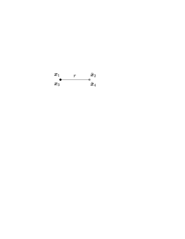
(a)

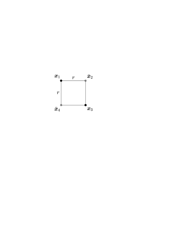
(b)

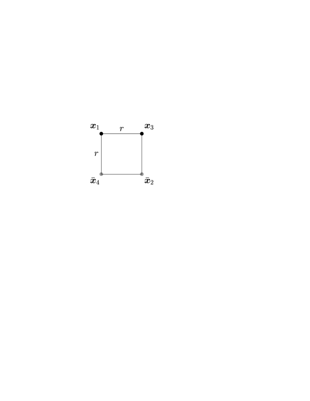
(c)

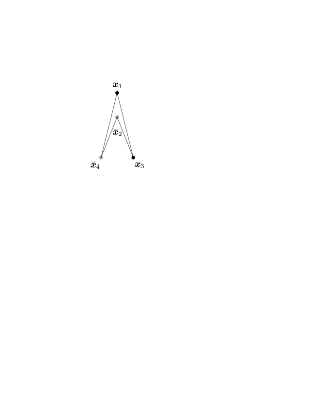
(d)

Figure 1: Special quadrupole configurations that we shall use to illustrate our general results. The dots represent the positions of the fermions in the transverse plane. (A bar on a transverse coordinate refers to an antiquark.) The lines have no physical meaning, they are meant only to delimitate the shape of the figures, in conformity with the names that we use to refer to them.

We shall pick the ‘line’ configuration, where we place the two quarks on top of each other and the same for the antiquarks (see Fig. 1.a), as our warm–up example. For this example, we shall perform in detail all the steps to be repeated for the general case in the next section. (The three other configurations in Fig. 1 will be studied in Sect. 4, as special limits of our general result for the quadrupole.) As obvious from Fig. 1.a, the ‘line’ configuration involves a single transverse scale $r$, which is the common size of the four $q\bar{q}$ pairs: $r_{12}=r_{14}=r_{23}=r_{34}\equiv r$. When applied to this configuration, the general evolution equation (10) reduces to

$$\frac{\partial\langle\hat{Q}_{\bm{x}_{1}\bm{x}_{2}\bm{x}_{1}\bm{x}_{2}}\rangle_{Y}}{\partial Y} = \frac{\bar{\alpha}}{\pi}\int_{\bm{z}}\mathcal{M}_{\bm{x}_{1}\bm{x}_{2}\bm{z}}\big{[}\langle\hat{S}_{\bm{x}_{1}\bm{z}}\rangle_{Y}\langle\hat{Q}_{\bm{z}\bm{x}_{2}\bm{x}_{1}\bm{x}_{2}}\rangle_{Y}+\langle\hat{S}_{\bm{z}\bm{x}_{2}}\rangle_{Y}\langle\hat{Q}_{\bm{x}_{1}\bm{z}\bm{x}_{1}\bm{x}_{2}}\rangle_{Y}$$ (6)

$$\qquad\qquad\qquad-\langle\hat{Q}_{\bm{x}_{1}\bm{x}_{2}\bm{x}_{1}\bm{x}_{2}}\rangle_{Y}-\langle\hat{S}_{\bm{x}_{1}\bm{x}_{2}}\rangle_{Y}^{2}\big{]}.$$

When the separation $r$ is much larger than $1/Q_{s}$, the virtual terms (the last two terms in Eq. (6)) dominate and give

$$\frac{\partial\langle\hat{Q}(r)\rangle_{Y}}{\partial Y}\simeq-2\bar{\alpha}\ln(r^{2}Q_{s}^{2})\,\big{[}\langle\hat{Q}(r)\rangle_{Y}+\langle\hat{S}(r)\rangle_{Y}^{2}\big{]}\,.$$ (7)

We have written the argument of the quadrupole simply as $\hat{Q}(r)$, because $r$ is the only independent transverse scale for this particular configuration. After also using Eq. (4), it turns out that this inhomogeneous equation admits a relatively simple solution, which is (for $Y\geq Y_{0}$)

$$\langle\hat{Q}(r)\rangle_{Y}=\langle\hat{S}(r)\rangle_{Y}^{2}\left[\frac{\langle\hat{Q}(r)\rangle_{Y_{0}}}{\langle\hat{S}(r)\rangle_{Y_{0}}^{2}}+\ln\frac{\langle\hat{S}(r)\rangle_{Y}^{2}}{\langle\hat{S}(r)\rangle_{Y_{0}}^{2}}\right]\qquad\mbox{(`line' in Fig.~{}\ref{Fig:configs}.a)}\,.$$ (8)

In view of its derivation above, one may expect this formula to hold only deeply at saturation, that is, for $Y>Y_{0}$, with $Y_{0}$ the rapidity at which saturation sets in on the given transverse scale $r$. But as a matter of facts, Eq. (8) is more general than that: it has also the right limit at weak scattering, in agreement with Eq. (2), and hence it provides a global approximation. To see that, let us study the weak scattering limit of Eq. (8), by writing $\langle\hat{S}(r)\rangle_{Y}=1-\langle\hat{T}(r)\rangle_{Y}$, with $\langle\hat{T}(r)\rangle_{Y}\ll 1$, and then expanding the r.h.s. to linear order in $\langle\hat{T}(r)\rangle_{Y}$. After doing that, one finds that the following relation is satisfied at $Y$, provided it was already satisfied at $Y_{0}$ :

$$\langle\hat{Q}(r)\rangle_{Y}\simeq 1-4\langle\hat{T}(r)\rangle_{Y}\,.$$ (9)

As anticipated, Eq. (9) is the correct weak–scattering limit for this particular configuration, as predicted by Eq. (2).

Eq. (8) can be further simplified if one assumes that the initial conditions at $Y_{0}$ are provided by the MV model at large $N_{c}$. Indeed, it is easy to check that Eq. (8) reduces to

$$\langle\hat{Q}(r)\rangle_{Y}=\langle\hat{S}(r)\rangle_{Y}^{2}\left[1+\ln{\langle\hat{S}(r)\rangle_{Y}^{2}}\right]\,,$$ (10)

provided the above formula already holds at the initial rapidity $Y_{0}$ — a property which is indeed satisfied within the MV model at large $N_{c}$.

To summarize, by using Eq. (10) together with a reasonable approximation for the dipole $S$–matrix $\langle\hat{S}(r)\rangle_{Y}$ — say, the solution to the BK equation with initial conditions provided by the large–$N_{c}$ version of the MV model — one obtains a unified description for (i) the initial conditions at low energy, (ii) the BFKL regime at high energy, and (iii) the approach towards the black disk limit at all the energies.

As demonstrated by the numerical analysis in Ref. Dumitru:2011vk , Eq. (10) agrees well with the numerical solution to the JIMWLK equation for this particular configuration. In the forthcoming section and in Appendix B, we shall generalize Eq. (8) to generic configurations for the quadrupole and the sextupole, and we shall also study some other particular configurations.

4 A global approximation for the quadrupole

We shall now extend the analysis in the previous section to a generic configuration for the quadrupole — that is, we shall study the approximation obtained by keeping only the virtual terms in Eq. (10). In line with our general strategy, we shall rely on this approximation, which is strictly speaking valid only in the vicinity of the black disk limit, in order to derive a functional relation between the quadrupole and the dipole, that will be then promoted to a global approximation.

After neglecting the ‘real’ terms and restricting the integrations over $\bm{z}$ to the regions yielding large logarithmic contributions, like in Eq. (3), we get

$$\frac{\partial\langle\hat{Q}_{\bm{x}_{1}\bm{x}_{2}\bm{x}_{3}\bm{x}_{4}}\rangle_{Y}}{\partial Y}\simeq\, - \frac{\bar{\alpha}}{2}\left[\ln(r_{12}^{2}Q_{s}^{2})+\ln(r_{34}^{2}Q_{s}^{2})+\ln(r_{14}^{2}Q_{s}^{2})+\ln(r_{23}^{2}Q_{s}^{2})\right]\langle\hat{Q}_{\bm{x}_{1}\bm{x}_{2}\bm{x}_{3}\bm{x}_{4}}\rangle_{Y}$$

$$- \frac{\bar{\alpha}}{2}\left[\ln(r_{12}^{2}Q_{s}^{2})+\ln(r_{34}^{2}Q_{s}^{2})-\ln(r_{13}^{2}Q_{s}^{2})-\ln(r_{24}^{2}Q_{s}^{2})\right]\langle\hat{S}_{\bm{x}_{1}\bm{x}_{2}}\rangle_{Y}\langle\hat{S}_{\bm{x}_{3}\bm{x}_{4}}\rangle_{Y}$$

$$- \frac{\bar{\alpha}}{2}\left[\ln(r_{14}^{2}Q_{s}^{2})+\ln(r_{23}^{2}Q_{s}^{2})-\ln(r_{13}^{2}Q_{s}^{2})-\ln(r_{24}^{2}Q_{s}^{2})\right]\langle\hat{S}_{\bm{x}_{3}\bm{x}_{2}}\rangle_{Y}\langle\hat{S}_{\bm{x}_{1}\bm{x}_{4}}\rangle_{Y},$$

where in writing the r.h.s. we have also factorized the 2–dipole $S$–matrix, as appropriate at large $N_{c}$. Now we can use Eq. (4) in order to express the logarithms in terms of the dipole $S$-matrix. The merit of that is three-fold. First, we can express the quadrupole in terms of the dipole without worrying about the explicit solution for the latter. Second, in order to get the dominant logarithmic contribution we do the same kind of approximation in both the dipole and the quadrupole equations since their structures are the same. Therefore we probably have better control than originally announced, that is, we have better accuracy than the one given by the leading logarithmic terms. Third, we do not really need to specify the energy dependence of $Q_{s}$ and thus the approach is fully valid even if we consider a running coupling scenario (at least in the case where $\bar{\alpha}$ is evaluated at $Q_{s}$). Thus, writing all logarithms in Eq. (4) terms of $S$ we have

$$\frac{\partial\langle\hat{Q}_{\bm{x}_{1}\bm{x}_{2}\bm{x}_{3}\bm{x}_{4}}\rangle_{Y}}{\partial Y} = \frac{1}{2}\left[\frac{\partial}{\partial Y}\ln\langle\hat{S}_{\bm{x}_{1}\bm{x}_{2}}\rangle_{Y}\langle\hat{S}_{\bm{x}_{3}\bm{x}_{2}}\rangle_{Y}\langle\hat{S}_{\bm{x}_{3}\bm{x}_{4}}\rangle_{Y}\langle\hat{S}_{\bm{x}_{1}\bm{x}_{4}}\rangle_{Y}\right]\langle\hat{Q}_{\bm{x}_{1}\bm{x}_{2}\bm{x}_{3}\bm{x}_{4}}\rangle_{Y}$$ (2)

$$+ \frac{1}{2}\left[\frac{\partial}{\partial Y}\ln\frac{\langle\hat{S}_{\bm{x}_{1}\bm{x}_{2}}\rangle_{Y}\langle\hat{S}_{\bm{x}_{3}\bm{x}_{4}}\rangle_{Y}}{\langle\hat{S}_{\bm{x}_{1}\bm{x}_{3}}\rangle_{Y}\langle\hat{S}_{\bm{x}_{2}\bm{x}_{4}}\rangle_{Y}}\right]\langle\hat{S}_{\bm{x}_{1}\bm{x}_{2}}\rangle_{Y}\langle\hat{S}_{\bm{x}_{3}\bm{x}_{4}}\rangle_{Y}$$

$$+ \frac{1}{2}\left[\frac{\partial}{\partial Y}\ln\frac{\langle\hat{S}_{\bm{x}_{1}\bm{x}_{4}}\rangle_{Y}\langle\hat{S}_{\bm{x}_{3}\bm{x}_{2}}\rangle_{Y}}{\langle\hat{S}_{\bm{x}_{1}\bm{x}_{3}}\rangle_{Y}\langle\hat{S}_{\bm{x}_{2}\bm{x}_{4}}\rangle_{Y}}\right]\langle\hat{S}_{\bm{x}_{1}\bm{x}_{4}}\rangle_{Y}\langle\hat{S}_{\bm{x}_{3}\bm{x}_{2}}\rangle_{Y}.$$

This is an ordinary first order inhomogeneous differential equation whose general solution is straightforward to find; it reads

$$\langle\hat{Q}_{\bm{x}_{1}\bm{x}_{2}\bm{x}_{3}\bm{x}_{4}}\rangle_{Y}=\sqrt{\langle\hat{S}_{\bm{x}_{1}\bm{x}_{2}}\rangle_{Y}\langle\hat{S}_{\bm{x}_{3}\bm{x}_{2}}\rangle_{Y}\langle\hat{S}_{\bm{x}_{3}\bm{x}_{4}}\rangle_{Y}\langle\hat{S}_{\bm{x}_{1}\bm{x}_{4}}\rangle_{Y}}\left[\frac{\langle\hat{Q}_{\bm{x}_{1}\bm{x}_{2}\bm{x}_{3}\bm{x}_{4}}\rangle_{Y_{0}}}{\sqrt{\langle\hat{S}_{\bm{x}_{1}\bm{x}_{2}}\rangle_{Y_{0}}\langle\hat{S}_{\bm{x}_{3}\bm{x}_{2}}\rangle_{Y_{0}}\langle\hat{S}_{\bm{x}_{3}\bm{x}_{4}}\rangle_{Y_{0}}\langle\hat{S}_{\bm{x}_{1}\bm{x}_{4}}\rangle_{Y_{0}}}}\right.$$

$$\quad\left.+\,\frac{1}{2}\,\int_{Y_{0}}^{Y}{\rm d}y\,\frac{\langle\hat{S}_{\bm{x}_{1}\bm{x}_{3}}\rangle_{y}\langle\hat{S}_{\bm{x}_{2}\bm{x}_{4}}\rangle_{y}}{\sqrt{\langle\hat{S}_{\bm{x}_{1}\bm{x}_{2}}\rangle_{y}\langle\hat{S}_{\bm{x}_{3}\bm{x}_{2}}\rangle_{y}\langle\hat{S}_{\bm{x}_{3}\bm{x}_{4}}\rangle_{y}\langle\hat{S}_{\bm{x}_{1}\bm{x}_{4}}\rangle_{y}}}\,\frac{\partial}{\partial y}\frac{\langle\hat{S}_{\bm{x}_{1}\bm{x}_{2}}\rangle_{y}\langle\hat{S}_{\bm{x}_{3}\bm{x}_{4}}\rangle_{y}+\langle\hat{S}_{\bm{x}_{1}\bm{x}_{4}}\rangle_{y}\langle\hat{S}_{\bm{x}_{3}\bm{x}_{2}}\rangle_{y}}{\langle\hat{S}_{\bm{x}_{1}\bm{x}_{3}}\rangle_{y}\langle\hat{S}_{\bm{x}_{2}\bm{x}_{4}}\rangle_{y}}\right]\!\!.$$ (3)

As explained in the Introduction, the above expression is guaranteed to be correct also for weak scattering, even though it has been obtained here via manipulations which are well justified only deeply at saturation. This is so since, at weak scattering, the relation between the quadrupole and the dipole becomes linear, cf. Eq. (2). Such a linear relation is then preserved by any evolution equation generated by a Hamiltonian — in particular, by the equations including only the virtual terms, which are generated, as we have seen, by a truncated version of the JIMWLK Hamiltonian (the first two terms in Eq. (2)). This argument about linearity is simple, but at the same time important for the present construction, so let us make a small digression in order to explain it better.

Consider a set of three operators, $\hat{A}$, $\hat{B}$, and $\hat{C}$, which obey a linear relation: $\hat{A}=c_{1}\hat{B}+c_{2}\hat{C}$. Also assume that the evolution of these operators with ‘time’ $Y$ is governed by some Hamiltonian $H$; e.g. $\partial_{Y}\hat{A}=H\hat{A}$. Then one can successively write

$$\frac{\partial\hat{A}}{\partial Y}\,=\,H\hat{A}\,=\,H\big{(}c_{1}\hat{B}+c_{2}\hat{C}\big{)}\,=\,c_{1}\frac{\partial\hat{B}}{\partial Y}\,+\,c_{2}\frac{\partial\hat{C}}{\partial Y}\,.$$ (4)

This equation implies that the linear relation $\hat{A}=c_{1}\hat{B}+c_{2}\hat{C}$ is preserved at any $Y$ provided it was satisfied at the initial ‘time’ $Y_{0}$. Note that specific form of $H$ was irrelevant for the above argument; all that matters is the fact that this is a linear operator.

Returning to the physics problem at hand, the relation (4) between the quadrupole and the dipole has been obtained by solving a Hamiltonian evolution equation. The corresponding Hamiltonian is incorrect in the dilute regime, where it would predict a wrong evolution for the quadrupole, or the dipole, taken separately. However, as a linear operator, it must preserve the linear relation (2) between the two operators $\hat{Q}$ and $\hat{S}$ which is valid in that regime. And indeed, it can be easily checked — by rewriting $\langle\hat{S}_{\bm{x}_{i}\bm{x}_{j}}\rangle_{y}=1-\langle\hat{T}_{\bm{x}_{i}\bm{x}_{j}}\rangle_{y}$ and then expanding the r.h.s. of Eq. (4) to linear order in the various $\langle\hat{T}_{\bm{x}_{i}\bm{x}_{j}}\rangle_{y}$’s — that Eq. (4) predicts the correct relation, Eq. (2), between the quadrupole and the dipole at weak scattering and at rapidity $Y$ provided this relation was already satisfied at the initial rapidity $Y_{0}$.

In view of the above, we conclude that Eq. (4), when used with a numerical solution of the BK equation (or some good approximation to it), provides a reliable approximation to the solution to the quadrupole equation which is valid in all regimes (at least for generic configurations, which are not very asymmetric). This solution provides a smooth (infinitely differentiable) interpolation between the BFKL solution in the weak scattering regime at $r_{ij}\ll 1/Q_{s}$ and the correct approach towards the black disk limit at $r_{ij}\gg 1/Q_{s}$.

The expression (4) has some other good properties. It is symmetric under the interchange of the two quarks (or the two antiquarks) at any $Y$, provided that this is true at the initial rapidity $Y_{0}$. This is a true property of the JIMWLK evolution at large-$N_{c}$, as it can be directly checked at the level of the evolution equations in Sect. 2. Furthermore, there is an interesting relation between Eq. (4) and the corresponding expression in the MV model JalilianMarian:2004da ; Dominguez:2011wm . To see this connection, it is useful to write the dipole $S$–matrix in the form

$$\langle\hat{S}_{\bm{x}_{i}\bm{x}_{j}}\rangle_{Y}={\rm e}^{-\Gamma_{Y}(\bm{x}_{i},\bm{x}_{j})}\langle\hat{S}_{\bm{x}_{i}\bm{x}_{j}}\rangle_{Y_{0}}.$$ (5)

Now, (4) becomes formally identical with the quadrupole formula in the MV model (for large $N_{c}$) provided one assumes $\Gamma_{Y}(\bm{x}_{i},\bm{x}_{j})$ to be a separable function of $Y$ and the transverse coordinates, plus an arbitrary function of $Y$. This property is certainly not satisfied in general, but it is locally satisfied under some approximations — e.g., in the window for extended geometric scaling, where $\Gamma_{Y}(r)\simeq(r^{2}Q_{s}^{2}(Y))^{\gamma_{s}}$ with $\gamma_{s}\approx 0.63$ (modulo more slowly varying logarithmic terms) Iancu:2002tr ; Mueller:2002zm ; Munier:2003vc , and deep at saturation where $\Gamma_{Y}(r)\simeq(1/2\omega)\ln^{2}[r^{2}Q_{s}^{2}(Y)]$ (cf. Eq. (5)). This is also fulfilled in some dipole models, like the GBW model GolecBiernat:1998js ; GolecBiernat:1999qd , where $\Gamma_{Y}(r)=r^{2}Q_{s}^{2}(Y)/4$. Assuming this to be the case, then it is possible to explicitly perform the integral over $y$ in Eq. (4) and thus obtain, after some algebraic manipulations,

$$\langle\hat{Q}_{\bm{x}_{1}\bm{x}_{2}\bm{x}_{3}\bm{x}_{4}}\rangle_{Y} = \frac{\Gamma_{Y}(\bm{x}_{1},\bm{x}_{2})+\Gamma_{Y}(\bm{x}_{3},\bm{x}_{4})-\Gamma_{Y}(\bm{x}_{1},\bm{x}_{3})-\Gamma_{Y}(\bm{x}_{2},\bm{x}_{4})}{\Gamma_{Y}(\bm{x}_{1},\bm{x}_{2})+\Gamma_{Y}(\bm{x}_{3},\bm{x}_{4})-\Gamma_{Y}(\bm{x}_{1},\bm{x}_{4})-\Gamma_{Y}(\bm{x}_{2},\bm{x}_{3})}\,{\langle\hat{S}_{\bm{x}_{1}\bm{x}_{2}}\rangle_{Y}\langle\hat{S}_{\bm{x}_{3}\bm{x}_{4}}\rangle_{Y}}$$ (6)

$$+ \frac{\Gamma_{Y}(\bm{x}_{1},\bm{x}_{4})+\Gamma_{Y}(\bm{x}_{2},\bm{x}_{3})-\Gamma_{Y}(\bm{x}_{1},\bm{x}_{3})-\Gamma_{Y}(\bm{x}_{2},\bm{x}_{4})}{\Gamma_{Y}(\bm{x}_{1},\bm{x}_{4})+\Gamma_{Y}(\bm{x}_{2},\bm{x}_{3})-\Gamma_{Y}(\bm{x}_{1},\bm{x}_{2})-\Gamma_{Y}(\bm{x}_{3},\bm{x}_{4})}\,{\langle\hat{S}_{\bm{x}_{1}\bm{x}_{4}}\rangle_{Y}\langle\hat{S}_{\bm{x}_{3}\bm{x}_{2}}\rangle_{Y}},$$

which is indeed the same as the corresponding expression in the MV model at large $N_{c}$ JalilianMarian:2004da ; Dominguez:2011wm . Notice that the quadrupole at $Y_{0}$ does not appear anymore since in writing Eq. (6) we have assumed that the latter is already valid at $Y_{0}$, as correct for initial conditions of the MV type.

Returning to the general formula (4), let us notice that there are special quadrupole configurations, like those shown in Fig. 1, which have enough symmetry for the integral over $y$ to be exactly doable, without additional assumptions. For instance, consider the case where all transverse separations between a quark and an antiquark are the same, that is $r_{12}=r_{34}=r_{14}=r_{32}\equiv r$. (This includes the ‘line’, Fig. 1.a, and also the first ‘square’, Fig. 1.b.) Then the integrand in Eq. (4) is a total derivative, so one easily finds

$$\langle\hat{Q}\rangle_{Y}=\langle\hat{S}(r)\rangle_{Y}^{2}\left[\frac{\langle\hat{Q}\rangle_{Y_{0}}}{\langle\hat{S}(r)\rangle_{Y_{0}}^{2}}+\ln\frac{\langle\hat{S}(r)\rangle_{Y}^{2}}{\langle\hat{S}(r_{13})\rangle_{Y}\langle\hat{S}(r_{24})\rangle_{Y}}-\ln\frac{\langle\hat{S}(r)\rangle_{Y_{0}}^{2}}{\langle\hat{S}(r_{13})\rangle_{Y_{0}}\langle\hat{S}(r_{24})\rangle_{Y_{0}}}\right].$$ (7)

The arguments of $\langle\hat{Q}\rangle_{Y}$, which here is a function of $r$, $r_{13}$, and $r_{24}$, are kept implicit.

The ‘line’ configuration in Fig. 1.a corresponds to $r_{13}=r_{24}=0$, and then Eq. (7) reduces to Eq. (10), as expected. As for the ‘square’ configuration in Fig. 1.b, one has $r_{13}=r_{24}=\sqrt{2}r$, so Eq. (7) gives

$$\langle\hat{Q}(r)\rangle_{Y}=\langle\hat{S}(r)\rangle_{Y}^{2}\left[\frac{\langle\hat{Q}(r)\rangle_{Y_{0}}}{\langle\hat{S}(r)\rangle_{Y_{0}}^{2}}+\ln\frac{\langle\hat{S}(r)\rangle_{Y}^{2}}{\langle\hat{S}(\sqrt{2}r)\rangle_{Y}^{2}}-\ln\frac{\langle\hat{S}(r)\rangle_{Y_{0}}^{2}}{\langle\hat{S}(\sqrt{2}r)\rangle_{Y_{0}}^{2}}\right]\,\,\mbox{(`square' in Fig.~{}\ref{Fig:configs}.b)}\,.$$ (8)

Notice that the above reduce to

$$\langle\hat{Q}(r)\rangle_{Y}=\langle\hat{S}(r)\rangle_{Y}^{2}\left[1+\ln\frac{\langle\hat{S}(r)\rangle_{Y}^{2}}{\langle\hat{S}(\sqrt{2}r)\rangle_{Y}^{2}}\right],$$ (9)

provided Eq. (9) is also valid at $Y_{0}$, as it is indeed the case in the MV model at large-$N_{c}$. More generally, Eq. (9) is valid at $Y$ even if it was not valid at $Y_{0}$ provided the scattering of a dipole with the given size $r$ was weak at $Y_{0}$. (But of course, the scattering can be strong at $Y>Y_{0}$ for the same size $r$.) Indeed, assuming that $\langle\hat{T}(r)\rangle_{Y_{0}}\ll 1$, and therefore also $\langle\hat{T}(\sqrt{2}r)\rangle_{Y_{0}}\ll 1$, it is straightforward to show that the pieces linear in $\langle\hat{T}\rangle_{Y_{0}}$ coming from the first and the last term of Eq. (8) mutually cancel and then Eq. (9) is again obtained.

In Ref. Dumitru:2011vk , Eq. (9) has been compared to the numerical solution to JIMWLK equation and the agreement appears to be remarkably good — actually, even better than for the ‘line’ configuration. Clearly, expressions like (9) or (10), which involve a single transverse scale $r$, exhibit geometric scaling in the same regime where the dipole does so. This feature too is in agreement with the numerical results in Ref. Dumitru:2011vk

A second class of configurations for which the integrand in Eq. (4) is a total derivative are those which are constrained by $r_{13}=r_{14}$ and $r_{23}=r_{24}$, whereas the two other separations $r_{12}$ and $r_{34}$ are left arbitrary. The two last configurations in Fig. 1 — the second ‘square’, Fig. 1.c, and the ‘double triangle’, Fig. 1.d — belong to this category. For any configuration in this class, Eq. (4) yields a very simple, factorized, expression

$$\langle\hat{Q}\rangle_{Y}=\frac{\langle\hat{Q}\rangle_{Y_{0}}}{\langle\hat{S}(r_{12})\rangle_{Y_{0}}\langle\hat{S}(r_{34})\rangle_{Y_{0}}}\,\langle\hat{S}(r_{12})\rangle_{Y}\langle\hat{S}(r_{34})\rangle_{Y},$$ (10)

which involves the unconstrained separations $r_{12}$ and $r_{34}$, but it is independent of the other ones (those which are constrained). As before, Eq. (10) reduces to an even simpler expression

$$\langle\hat{Q}\rangle_{Y}=\langle\hat{S}(r_{12})\rangle_{Y}\langle\hat{S}(r_{34})\rangle_{Y},$$ (11)

provided this last formula holds already at $Y_{0}$ (a property which, once again, is satisfied within the MV model at large $N_{c}$). In particular, for the second ‘square’ configuration in Fig. 1.c, one has $r_{13}=r_{14}=r_{23}=r_{24}\equiv r$ and $r_{12}=r_{34}=\sqrt{2}\,r$, and Eq. (11) gives

$$\langle\hat{Q}(r)\rangle_{Y}\,=\,\langle\hat{S}(\sqrt{2}\,r)\rangle_{Y}^{2}\qquad\mbox{(`square' in Fig.~{}\ref{Fig:configs}.c)}\,.$$ (12)

But the most interesting configuration in our opinion is the last one in Fig. 1: the ‘double triangle’. What is remarkable about this configuration is the fact that the separation between the $q\bar{q}$ pair $(\bm{x}_{1},\bm{x}_{2})$ and the second $q\bar{q}$ pair $(\bm{x}_{3},\bm{x}_{4})$ can be made arbitrary, yet the corresponding $S$–matrix in Eq. (10) is independent of this separation. In particular, so long as $r_{12}$ and $r_{34}$ are much smaller than $1/Q_{s}$, the scattering of the quadrupole as a whole remains weak independently of the distance $\sim r_{14}$ separating the two pairs — including in the case where $r_{14}\gg 1/Q_{s}(Y)$. This may look counterintuitive since normally one expects the scattering to be strong whenever the separation between color charges is of order $1/Q_{s}$ or larger. However, we believe that this result can be physically understood as follows: when the two quark–antiquark pairs $(\bm{x}_{1},\bm{x}_{2})$ and respectively $(\bm{x}_{3},\bm{x}_{4})$ are individually small, whereas the distance $\sim r_{14}$ between them is of order $1/Q_{s}$ or larger, the color exchanges between the two pairs are strongly suppressed by saturation; then, the color charges compensates locally, within each of the small $q\bar{q}$ pairs, which therefore behave like two individual dipoles. In view of this argument, the factorized structure of Eq. (10) looks quite natural. It would be very interesting to verify this formula via numerical simulations of the JIMWLK evolution, along the lines in Ref. Dumitru:2011vk .

Appendix A The evolution equation for the quadrupole

In this section, we shall present a particularly streamlined derivation of the evolution equation for the quadrupole, using the ‘dipole’ version of the JIMWLK Hamiltonian in Eq. (2). (An alternative derivation can be found in Ref. Dominguez:2011gc .)

For pedagogy, we shall first derive the evolution equation for a color dipole, that is, the 2–point function of the Wilson lines shown in Eq. (5). The action of the functional derivative on these Wilson lines is computed according to Eq. (8), thus yielding

$$\frac{\delta}{\delta\alpha^{a}_{\bm{u}}}\,\frac{\delta}{\delta\alpha^{b}_{\bm{v}}}\,V^{\dagger}_{\bm{x}_{1}}V_{\bm{x}_{2}}\rightarrow g^{2}\delta_{\bm{x}_{1}\bm{u}}\delta_{\bm{x}_{2}\bm{v}}\,t^{a}V_{\bm{x}_{1}}^{\dagger}V_{\bm{x}_{2}}t^{b}+g^{2}\delta_{\bm{x}_{1}\bm{v}}\delta_{\bm{x}_{2}\bm{u}}\,t^{b}V_{\bm{x}_{1}}^{\dagger}V_{\bm{x}_{2}}t^{a},$$ (13)

where in writing the r.h.s. we have dropped some terms proportional to $\delta_{\bm{u}\bm{v}}$ since the kernel $\mathcal{M}_{\bm{u}\bm{v}\bm{z}}$ vanishes when $\bm{u}=\bm{v}$.

Consider the first term in the parenthesis of Eq. (2), that is, the identity matrix. For it, both terms arising from Eq. (13) contribute equally and together yield the following contribution to $H\hat{S}_{\bm{x}_{1}\bm{x}_{2}}$ :

$$-\frac{N_{c}^{2}-1}{2N_{c}^{2}}\,\frac{\bar{\alpha}}{2\pi}\,\int\limits_{\bm{z}}\mathcal{M}_{\bm{x}_{1}\bm{x}_{2}\bm{z}}\,\hat{S}_{\bm{x}_{1}\bm{x}_{2}},$$ (14)

where we have also used $t^{a}t^{a}=(N_{c}^{2}-1)/2N_{c}$. Next consider the contribution coming from the second term in the parenthesis of Eq. (2). After expressing adjoint Wilson lines in terms of fundamental ones according to

$$\big{(}\widetilde{V}^{\dagger}\big{)}^{ac}t^{a}=\widetilde{V}^{cb}t^{b}=V^{\dagger}t^{c}\,V,$$ (15)

it becomes straightforward to show that this second term yields the same contribution as the first one, that is, Eq. (14). The third term in the Hamiltonian leads to contributions like

$$\big{(}\widetilde{V}_{\bm{x}_{1}}^{\dagger}\big{)}^{ac}\,\widetilde{V}_{\bm{z}}^{cb}\,{\rm tr}\big{(}t^{a}\,V_{\bm{x}_{1}}^{\dagger}V_{\bm{x}_{2}}t^{b}\big{)}={\rm tr}\big{(}V_{\bm{x}_{1}}^{\dagger}\,t^{c}\,V_{\bm{x}_{2}}V_{\bm{z}}^{\dagger}\,t^{c}\,V_{\bm{z}}\big{)}.$$ (16)

By using the Fierz identity

$${\rm tr}\big{(}t^{a}A\,t^{a}B\big{)}=\frac{1}{2}\,{\rm tr}A\,{\rm tr}B-\frac{1}{2N_{c}}\,{\rm tr}(AB),$$ (17)

we find that the corresponding contribution to $H\hat{S}_{\bm{x}_{1}\bm{x}_{2}}$, which also is equal to the one coming from the fourth term in Eq. (2), is

$$\frac{1}{2}\,\frac{\bar{\alpha}}{2\pi}\,\int\limits_{\bm{z}}\mathcal{M}_{\bm{x}_{1}\bm{x}_{2}\bm{z}}\Big{(}\hat{S}_{\bm{x}_{1}\bm{z}}\hat{S}_{\bm{z}\bm{x}_{2}}-\frac{1}{N_{c}^{2}}\,\hat{S}_{\bm{x}_{1}\bm{x}_{2}}\Big{)}.$$ (18)

Putting all contributions together and averaging over the color field of the target, we arrive at the dipole equation shown in Eq. (9).

Now let us turn our attention to the object of interest, the quadrupole operator, as defined in Eq. (6). The two functional derivatives can now act on 6 pairs of Wilson lines while the remaining two Wilson lines are simply ‘spectators’. Just for the sake of illustration we shall give here some intermediate steps for the terms that arise when the ‘active’ pair is the one composed of the two quarks at $\bm{x}_{1}$ and $\bm{x}_{3}$. Acting on the respective Wilson lines with the first term of the Hamiltonian, we find

$$\frac{g^{2}}{8\pi^{3}N_{c}}\int_{\bm{z}}\mathcal{M}_{\bm{x}_{1}\bm{x}_{3}\bm{z}}{\rm tr}(t^{a}{V}^{\dagger}_{\bm{x}_{1}}{V}_{\bm{x}_{2}}t^{a}{V}^{\dagger}_{\bm{x}_{3}}{V}_{\bm{x}_{4}}),$$

which after simple manipulations using the Fierz identity in Eq. (17) leads to

$$\frac{\bar{\alpha}}{4\pi}\int_{\bm{z}}\mathcal{M}_{\bm{x}_{1}\bm{x}_{3}\bm{z}}\Big{(}\hat{S}_{\bm{x}_{1}\bm{x}_{2}}\hat{S}_{\bm{x}_{3}\bm{x}_{4}}-\frac{1}{N_{c}^{2}}\,\hat{Q}_{\bm{x}_{1}\bm{x}_{2}\bm{x}_{3}\bm{x}_{4}}\Big{)}.$$ (19)

Acting with the second term of the Hamiltonian we obtain

$$\frac{g^{2}}{16\pi^{3}N_{c}}\int_{\bm{z}}\mathcal{M}_{\bm{x}_{1}\bm{x}_{3}\bm{z}}\left[\big{(}\widetilde{V}_{\bm{x}_{1}}^{\dagger}\big{)}^{ac}\widetilde{V}_{\bm{x}_{3}}^{cb}\,{\rm tr}(t^{a}{V}^{\dagger}_{\bm{x}_{1}}{V}_{\bm{x}_{2}}t^{b}{V}^{\dagger}_{\bm{x}_{3}}{V}_{\bm{x}_{4}})+\big{(}\widetilde{V}_{\bm{x}_{3}}^{\dagger}\big{)}^{ac}\widetilde{V}_{\bm{x}_{1}}^{cb}\,{\rm tr}(t^{b}{V}^{\dagger}_{\bm{x}_{1}}{V}_{\bm{x}_{2}}t^{a}{V}^{\dagger}_{\bm{x}_{3}}{V}_{\bm{x}_{4}})\right],$$

and by also making use of Eq. (15) we are lead to

$$\frac{\bar{\alpha}}{4\pi}\int_{\bm{z}}\mathcal{M}_{\bm{x}_{1}\bm{x}_{3}\bm{z}}\Big{(}\hat{S}_{\bm{x}_{3}\bm{x}_{2}}\hat{S}_{\bm{x}_{1}\bm{x}_{4}}-\frac{1}{N_{c}^{2}}\,\hat{Q}_{\bm{x}_{1}\bm{x}_{2}\bm{x}_{3}\bm{x}_{4}}\Big{)}.$$ (20)

The action of the third term of the Hamiltonian gives

$$-\frac{g^{2}}{16\pi^{3}N_{c}}\int_{\bm{z}}\mathcal{M}_{\bm{x}_{1}\bm{x}_{3}\bm{z}}\left[\big{(}\widetilde{V}_{\bm{x}_{1}}^{\dagger}\big{)}^{ac}\widetilde{V}_{\bm{z}}^{cb}\,{\rm tr}(t^{a}{V}^{\dagger}_{\bm{x}_{1}}{V}_{\bm{x}_{2}}t^{b}{V}^{\dagger}_{\bm{x}_{3}}{V}_{\bm{x}_{4}})+\big{(}\widetilde{V}_{\bm{x}_{3}}^{\dagger}\big{)}^{ac}\widetilde{V}_{\bm{z}}^{cb}\,{\rm tr}(t^{b}{V}^{\dagger}_{\bm{x}_{1}}{V}_{\bm{x}_{2}}t^{a}{V}^{\dagger}_{\bm{x}_{3}}{V}_{\bm{x}_{4}})\right],$$

leading to

$$-\frac{\bar{\alpha}}{8\pi}\int_{\bm{z}}\mathcal{M}_{\bm{x}_{1}\bm{x}_{3}\bm{z}}\Big{(}\hat{S}_{\bm{z}\bm{x}_{2}}\hat{Q}_{\bm{x}_{1}\bm{z}\bm{x}_{3}\bm{x}_{4}}+\hat{S}_{\bm{z}\bm{x}_{4}}\hat{Q}_{\bm{x}_{1}\bm{x}_{2}\bm{x}_{3}\bm{z}}-\frac{2}{N_{c}^{2}}\,\hat{Q}_{\bm{x}_{1}\bm{x}_{2}\bm{x}_{3}\bm{x}_{4}}\Big{)}.$$ (21)

Finally the action of the fourth term in the Hamiltonian gives

$$-\frac{g^{2}}{16\pi^{3}N_{c}}\int_{\bm{z}}\mathcal{M}_{\bm{x}_{1}\bm{x}_{3}\bm{z}}\left[\big{(}\widetilde{V}_{\bm{z}}^{\dagger}\big{)}^{ac}\widetilde{V}_{\bm{x}_{3}}^{cb}\,{\rm tr}(t^{a}{V}^{\dagger}_{\bm{x}_{1}}{V}_{\bm{x}_{2}}t^{b}{V}^{\dagger}_{\bm{x}_{3}}{V}_{\bm{x}_{4}})+\big{(}\widetilde{V}_{\bm{z}}^{\dagger}\big{)}^{ac}\widetilde{V}_{\bm{x}_{1}}^{cb}\,{\rm tr}(t^{b}{V}^{\dagger}_{\bm{x}_{1}}{V}_{\bm{x}_{2}}t^{a}{V}^{\dagger}_{\bm{x}_{3}}{V}_{\bm{x}_{4}})\right],$$

yielding the same result as shown in Eq. (21). Putting together all the contributions, we see that the terms explicitly suppressed by $1/N_{c}^{2}$ cancel each other, as anticipated. Thus, the action of the Hamiltonian on the pair made with the two quarks at $\bm{x}_{1}$ and $\bm{x}_{3}$ gives

$$-\frac{\bar{\alpha}}{4\pi}\int_{\bm{z}}\mathcal{M}_{\bm{x}_{1}\bm{x}_{3}\bm{z}}\big{(}\hat{S}_{\bm{z}\bm{x}_{2}}\hat{Q}_{\bm{x}_{1}\bm{z}\bm{x}_{3}\bm{x}_{4}}+\hat{S}_{\bm{z}\bm{x}_{4}}\hat{Q}_{\bm{x}_{1}\bm{x}_{2}\bm{x}_{3}\bm{z}}-\hat{S}_{\bm{x}_{1}\bm{x}_{2}}\hat{S}_{\bm{x}_{3}\bm{x}_{4}}-\hat{S}_{\bm{x}_{3}\bm{x}_{2}}\hat{S}_{\bm{x}_{1}\bm{x}_{4}}\big{)}.$$ (22)

Similarly, when acting on the quark and the antiquark at $\bm{x}_{1}$ and $\bm{x}_{2}$ respectively, we obtain

$$\frac{\bar{\alpha}}{4\pi}\int_{\bm{z}}\mathcal{M}_{\bm{x}_{1}\bm{x}_{2}\bm{z}}\big{(}\hat{S}_{\bm{x}_{1}\bm{z}}\hat{Q}_{\bm{z}\bm{x}_{2}\bm{x}_{3}\bm{x}_{4}}+\hat{S}_{\bm{z}\bm{x}_{2}}\hat{Q}_{\bm{x}_{1}\bm{z}\bm{x}_{3}\bm{x}_{4}}-\hat{Q}_{\bm{x}_{1}\bm{x}_{2}\bm{x}_{3}\bm{x}_{4}}-\hat{S}_{\bm{x}_{1}\bm{x}_{2}}\hat{S}_{\bm{x}_{3}\bm{x}_{4}}\big{)}.$$ (23)

The action of the Hamiltonian on the other possible pairs of Wilson lines is obtained via appropriate permutations in either Eq. (22) or Eq. (23). Putting all terms together and averaging over the target field, we arrive at the evolution equation shown in Eq. (10) in the main text.

Appendix B The sextupole

In order to demonstrate the generality of our procedure, we shall succinctly present here the corresponding analysis for the next non–trivial high–point correlator, which is the sextupole defined in Eq. (7). The respective evolution equation has not been yet presented in the literature, thus we have derived it on this occasion. We shall not give here the details of the derivation, since this is merely a lengthy but straightforward repetition of the manipulations shown in the previous Appendix. This is the final result:

$$\frac{\partial\langle\hat{S}_{\bm{x}_{1}\bm{x}_{2}\bm{x}_{3}\bm{x}_{4}\bm{x}_{5}\bm{x}_{6}}^{(6)}\rangle_{Y}}{\partial Y} = \frac{\bar{\alpha}}{4\pi}\int_{\bm{z}}\Big{[}(\mathcal{M}_{\bm{x}_{1}\bm{x}_{2}\bm{z}}+\mathcal{M}_{\bm{x}_{1}\bm{x}_{6}\bm{z}}-\mathcal{M}_{\bm{x}_{2}\bm{x}_{6}\bm{z}})\langle\hat{S}_{\bm{x}_{1}\bm{z}}\hat{S}_{\bm{z}\bm{x}_{2}\bm{x}_{3}\bm{x}_{4}\bm{x}_{5}\bm{x}_{6}}^{(6)}\rangle_{Y}$$ (24)

$$+ (\mathcal{M}_{\bm{x}_{1}\bm{x}_{2}\bm{z}}+\mathcal{M}_{\bm{x}_{2}\bm{x}_{3}\bm{z}}-\mathcal{M}_{\bm{x}_{1}\bm{x}_{3}\bm{z}})\langle\hat{S}_{\bm{z}\bm{x}_{2}}\hat{S}_{\bm{x}_{1}\bm{z}\bm{x}_{3}\bm{x}_{4}\bm{x}_{5}\bm{x}_{6}}^{(6)}\rangle_{Y}$$

$$+ (\mathcal{M}_{\bm{x}_{2}\bm{x}_{3}\bm{z}}+\mathcal{M}_{\bm{x}_{3}\bm{x}_{4}\bm{z}}-\mathcal{M}_{\bm{x}_{2}\bm{x}_{4}\bm{z}})\langle\hat{S}_{\bm{x}_{3}\bm{z}}\hat{S}_{\bm{x}_{1}\bm{x}_{2}\bm{z}\bm{x}_{4}\bm{x}_{5}\bm{x}_{6}}^{(6)}\rangle_{Y}$$

$$+ (\mathcal{M}_{\bm{x}_{3}\bm{x}_{4}\bm{z}}+\mathcal{M}_{\bm{x}_{4}\bm{x}_{5}\bm{z}}-\mathcal{M}_{\bm{x}_{3}\bm{x}_{5}\bm{z}})\langle\hat{S}_{\bm{z}\bm{x}_{4}}\hat{S}_{\bm{x}_{1}\bm{x}_{2}\bm{x}_{3}\bm{z}\bm{x}_{5}\bm{x}_{6}}^{(6)}\rangle_{Y}$$

$$+ (\mathcal{M}_{\bm{x}_{4}\bm{x}_{5}\bm{z}}+\mathcal{M}_{\bm{x}_{5}\bm{x}_{6}\bm{z}}-\mathcal{M}_{\bm{x}_{4}\bm{x}_{6}\bm{z}})\langle\hat{S}_{\bm{x}_{5}\bm{z}}\hat{S}_{\bm{x}_{1}\bm{x}_{2}\bm{x}_{3}\bm{x}_{4}\bm{z}\bm{x}_{6}}^{(6)}\rangle_{Y}$$

$$+ (\mathcal{M}_{\bm{x}_{1}\bm{x}_{6}\bm{z}}+\mathcal{M}_{\bm{x}_{5}\bm{x}_{6}\bm{z}}-\mathcal{M}_{\bm{x}_{1}\bm{x}_{5}\bm{z}})\langle\hat{S}_{\bm{z}\bm{x}_{6}}\hat{S}_{\bm{x}_{1}\bm{x}_{2}\bm{x}_{3}\bm{x}_{4}\bm{x}_{5}\bm{z}}^{(6)}\rangle_{Y}$$

$$+ (\mathcal{M}_{\bm{x}_{1}\bm{x}_{4}\bm{z}}+\mathcal{M}_{\bm{x}_{3}\bm{x}_{6}\bm{z}}-\mathcal{M}_{\bm{x}_{1}\bm{x}_{3}\bm{z}}-\mathcal{M}_{\bm{x}_{4}\bm{x}_{6}\bm{z}})\langle\hat{Q}_{\bm{x}_{1}\bm{x}_{2}\bm{x}_{3}\bm{z}}\hat{Q}_{\bm{z}\bm{x}_{4}\bm{x}_{5}\bm{x}_{6}}\rangle_{Y}$$

$$+ (\mathcal{M}_{\bm{x}_{2}\bm{x}_{5}\bm{z}}+\mathcal{M}_{\bm{x}_{3}\bm{x}_{6}\bm{z}}-\mathcal{M}_{\bm{x}_{3}\bm{x}_{5}\bm{z}}-\mathcal{M}_{\bm{x}_{2}\bm{x}_{6}\bm{z}})\langle\hat{Q}_{\bm{x}_{3}\bm{x}_{4}\bm{x}_{5}\bm{z}}\hat{Q}_{\bm{z}\bm{x}_{6}\bm{x}_{1}\bm{x}_{2}}\rangle_{Y}$$

$$+ (\mathcal{M}_{\bm{x}_{1}\bm{x}_{4}\bm{z}}+\mathcal{M}_{\bm{x}_{2}\bm{x}_{5}\bm{z}}-\mathcal{M}_{\bm{x}_{1}\bm{x}_{5}\bm{z}}-\mathcal{M}_{\bm{x}_{2}\bm{x}_{4}\bm{z}})\langle\hat{Q}_{\bm{x}_{5}\bm{x}_{6}\bm{x}_{1}\bm{z}}\hat{Q}_{\bm{z}\bm{x}_{2}\bm{x}_{3}\bm{x}_{4}}\rangle_{Y}$$

$$- (\mathcal{M}_{\bm{x}_{1}\bm{x}_{2}\bm{z}}+\mathcal{M}_{\bm{x}_{2}\bm{x}_{3}\bm{z}}+\mathcal{M}_{\bm{x}_{3}\bm{x}_{4}\bm{z}}+\mathcal{M}_{\bm{x}_{4}\bm{x}_{5}\bm{z}}+\mathcal{M}_{\bm{x}_{5}\bm{x}_{6}\bm{z}}+\mathcal{M}_{\bm{x}_{6}\bm{x}_{1}\bm{z}})\langle\hat{S}_{\bm{x}_{1}\bm{x}_{2}\bm{x}_{3}\bm{x}_{4}\bm{x}_{5}\bm{x}_{6}}^{(6)}\rangle_{Y}$$

$$- (\mathcal{M}_{\bm{x}_{1}\bm{x}_{2}\bm{z}}+\mathcal{M}_{\bm{x}_{3}\bm{x}_{6}\bm{z}}-\mathcal{M}_{\bm{x}_{1}\bm{x}_{3}\bm{z}}-\mathcal{M}_{\bm{x}_{2}\bm{x}_{6}\bm{z}})\langle\hat{S}_{\bm{x}_{1}\bm{x}_{2}}\hat{Q}_{\bm{x}_{3}\bm{x}_{4}\bm{x}_{5}\bm{x}_{6}}\rangle_{Y}$$

$$- (\mathcal{M}_{\bm{x}_{1}\bm{x}_{4}\bm{z}}+\mathcal{M}_{\bm{x}_{2}\bm{x}_{3}\bm{z}}-\mathcal{M}_{\bm{x}_{1}\bm{x}_{3}\bm{z}}-\mathcal{M}_{\bm{x}_{2}\bm{x}_{4}\bm{z}})\langle\hat{S}_{\bm{x}_{3}\bm{x}_{2}}\hat{Q}_{\bm{x}_{1}\bm{x}_{4}\bm{x}_{5}\bm{x}_{6}}\rangle_{Y}$$

$$- (\mathcal{M}_{\bm{x}_{3}\bm{x}_{4}\bm{z}}+\mathcal{M}_{\bm{x}_{2}\bm{x}_{5}\bm{z}}-\mathcal{M}_{\bm{x}_{2}\bm{x}_{4}\bm{z}}-\mathcal{M}_{\bm{x}_{3}\bm{x}_{5}\bm{z}})\langle\hat{S}_{\bm{x}_{3}\bm{x}_{4}}\hat{Q}_{\bm{x}_{1}\bm{x}_{2}\bm{x}_{5}\bm{x}_{6}}\rangle_{Y}$$

$$- (\mathcal{M}_{\bm{x}_{3}\bm{x}_{6}\bm{z}}+\mathcal{M}_{\bm{x}_{4}\bm{x}_{5}\bm{z}}-\mathcal{M}_{\bm{x}_{3}\bm{x}_{5}\bm{z}}-\mathcal{M}_{\bm{x}_{4}\bm{x}_{6}\bm{z}})\langle\hat{S}_{\bm{x}_{5}\bm{x}_{4}}\hat{Q}_{\bm{x}_{1}\bm{x}_{2}\bm{x}_{3}\bm{x}_{6}}\rangle_{Y}$$

$$- (\mathcal{M}_{\bm{x}_{1}\bm{x}_{4}\bm{z}}+\mathcal{M}_{\bm{x}_{5}\bm{x}_{6}\bm{z}}-\mathcal{M}_{\bm{x}_{1}\bm{x}_{5}\bm{z}}-\mathcal{M}_{\bm{x}_{4}\bm{x}_{6}\bm{z}})\langle\hat{S}_{\bm{x}_{5}\bm{x}_{6}}\hat{Q}_{\bm{x}_{1}\bm{x}_{2}\bm{x}_{3}\bm{x}_{4}}\rangle_{Y}$$

$$- (\mathcal{M}_{\bm{x}_{1}\bm{x}_{6}\bm{z}}+\mathcal{M}_{\bm{x}_{2}\bm{x}_{5}\bm{z}}-\mathcal{M}_{\bm{x}_{1}\bm{x}_{5}\bm{z}}-\mathcal{M}_{\bm{x}_{2}\bm{x}_{6}\bm{z}})\langle\hat{S}_{\bm{x}_{1}\bm{x}_{6}}\hat{Q}_{\bm{x}_{3}\bm{x}_{4}\bm{x}_{5}\bm{x}_{2}}\rangle_{Y}\Big{]}.$$

We notice that all the subleading terms of relative order $1/N_{c}^{2}$ have canceled in the final equation, as expected for a single trace operator. As a cross check, one can see that when choosing, for example, $\bm{x}_{5}=\bm{x}_{6}$, the above equation reduces to the quadrupole equation (10).

The subsequent manipulations follow the general procedure outlined in Sect. 4. First, one separates the ‘virtual’ terms in the r.h.s. of Eq. (24), that is, the terms in which the integration variable $\bm{z}$ appears only in the dipole kernel, but not in the correlation functions; these are the terms proportional to $\langle\hat{S}^{(6)}\rangle_{Y}$ and to $\langle\hat{S}\hat{Q}\rangle_{Y}\simeq\langle\hat{S}\rangle_{Y}\langle\hat{Q}\rangle_{Y}$. Then in evaluating the integrals over $\bm{z}$, one keeps only the dominant logarithmic contributions and use Eq. (4) to express the logarithms in term of the dipole derivative. We thus arrive at an ordinary first order inhomogeneous differential equation whose solution is

$$\langle\hat{S}_{\bm{x}_{1}\bm{x}_{2}\bm{x}_{3}\bm{x}_{4}\bm{x}_{5}\bm{x}_{6}}^{(6)}\rangle_{Y} = \sqrt{\langle\hat{S}_{\bm{x}_{1}\bm{x}_{2}}\rangle_{Y}\langle\hat{S}_{\bm{x}_{3}\bm{x}_{2}}\rangle_{Y}\langle\hat{S}_{\bm{x}_{3}\bm{x}_{4}}\rangle_{Y}\langle\hat{S}_{\bm{x}_{5}\bm{x}_{4}}\rangle_{Y}\langle\hat{S}_{\bm{x}_{5}\bm{x}_{6}}\rangle_{Y}\langle\hat{S}_{\bm{x}_{1}\bm{x}_{6}}\rangle_{Y}}$$ (25)

$$\ \mspace{-2.0mu}\times\mspace{-2.0mu}\left\{\frac{\langle\hat{S}_{\bm{x}_{1}\bm{x}_{2}\bm{x}_{3}\bm{x}_{4}\bm{x}_{5}\bm{x}_{6}}^{(6)}\rangle_{Y_{0}}}{\sqrt{\langle\hat{S}_{\bm{x}_{1}\bm{x}_{2}}\rangle_{Y_{0}}\langle\hat{S}_{\bm{x}_{3}\bm{x}_{2}}\rangle_{Y_{0}}\langle\hat{S}_{\bm{x}_{3}\bm{x}_{4}}\rangle_{Y_{0}}\langle\hat{S}_{\bm{x}_{5}\bm{x}_{4}}\rangle_{Y_{0}}\langle\hat{S}_{\bm{x}_{5}\bm{x}_{6}}\rangle_{Y_{0}}\langle\hat{S}_{\bm{x}_{1}\bm{x}_{6}}\rangle_{Y_{0}}}}\right.$$

$$\hskip 8.5359pt+\frac{1}{2}\,\int_{Y_{0}}^{Y}{\rm d}y\,\frac{1}{\sqrt{\langle\hat{S}_{\bm{x}_{1}\bm{x}_{2}}\rangle_{y}\langle\hat{S}_{\bm{x}_{3}\bm{x}_{2}}\rangle_{y}\langle\hat{S}_{\bm{x}_{3}\bm{x}_{4}}\rangle_{y}\langle\hat{S}_{\bm{x}_{5}\bm{x}_{4}}\rangle_{y}\langle\hat{S}_{\bm{x}_{5}\bm{x}_{6}}\rangle_{y}\langle\hat{S}_{\bm{x}_{1}\bm{x}_{6}}\rangle_{y}}}$$

$$\hskip 17.07182pt\mspace{-2.0mu}\times\mspace{-2.0mu}\Bigg{[}\langle\hat{S}_{\bm{x}_{1}\bm{x}_{2}}\rangle_{y}\langle\hat{Q}_{\bm{x}_{3}\bm{x}_{4}\bm{x}_{5}\bm{x}_{6}}\rangle_{y}\,\frac{\partial}{\partial y}\ln\frac{\langle\hat{S}_{\bm{x}_{1}\bm{x}_{2}}\rangle_{y}\langle\hat{S}_{\bm{x}_{3}\bm{x}_{6}}\rangle_{y}}{\langle\hat{S}_{\bm{x}_{1}\bm{x}_{3}}\rangle_{y}\langle\hat{S}_{\bm{x}_{2}\bm{x}_{6}}\rangle_{y}}$$

$$\hskip 22.76228pt+\langle\hat{S}_{\bm{x}_{3}\bm{x}_{2}}\rangle_{y}\langle\hat{Q}_{\bm{x}_{1}\bm{x}_{4}\bm{x}_{5}\bm{x}_{6}}\rangle_{y}\,\frac{\partial}{\partial y}\ln\frac{\langle\hat{S}_{\bm{x}_{3}\bm{x}_{2}}\rangle_{y}\langle\hat{S}_{\bm{x}_{1}\bm{x}_{4}}\rangle_{y}}{\langle\hat{S}_{\bm{x}_{1}\bm{x}_{3}}\rangle_{y}\langle\hat{S}_{\bm{x}_{2}\bm{x}_{4}}\rangle_{y}}$$

$$\hskip 22.76228pt+\langle\hat{S}_{\bm{x}_{3}\bm{x}_{4}}\rangle_{y}\langle\hat{Q}_{\bm{x}_{1}\bm{x}_{2}\bm{x}_{5}\bm{x}_{6}}\rangle_{y}\,\frac{\partial}{\partial y}\ln\frac{\langle\hat{S}_{\bm{x}_{3}\bm{x}_{4}}\rangle_{y}\langle\hat{S}_{\bm{x}_{5}\bm{x}_{2}}\rangle_{y}}{\langle\hat{S}_{\bm{x}_{2}\bm{x}_{4}}\rangle_{y}\langle\hat{S}_{\bm{x}_{3}\bm{x}_{5}}\rangle_{y}}$$

$$\hskip 22.76228pt+\langle\hat{S}_{\bm{x}_{5}\bm{x}_{4}}\rangle_{y}\langle\hat{Q}_{\bm{x}_{1}\bm{x}_{2}\bm{x}_{3}\bm{x}_{6}}\rangle_{y}\,\frac{\partial}{\partial y}\ln\frac{\langle\hat{S}_{\bm{x}_{5}\bm{x}_{4}}\rangle_{y}\langle\hat{S}_{\bm{x}_{3}\bm{x}_{6}}\rangle_{y}}{\langle\hat{S}_{\bm{x}_{3}\bm{x}_{5}}\rangle_{y}\langle\hat{S}_{\bm{x}_{4}\bm{x}_{6}}\rangle_{y}}$$

$$\hskip 22.76228pt+\langle\hat{S}_{\bm{x}_{5}\bm{x}_{6}}\rangle_{y}\langle\hat{Q}_{\bm{x}_{1}\bm{x}_{2}\bm{x}_{3}\bm{x}_{4}}\rangle_{y}\,\frac{\partial}{\partial y}\ln\frac{\langle\hat{S}_{\bm{x}_{5}\bm{x}_{6}}\rangle_{y}\langle\hat{S}_{\bm{x}_{1}\bm{x}_{4}}\rangle_{y}}{\langle\hat{S}_{\bm{x}_{1}\bm{x}_{5}}\rangle_{y}\langle\hat{S}_{\bm{x}_{4}\bm{x}_{6}}\rangle_{y}}$$

$$\hskip 22.76228pt+\!\left.\langle\hat{S}_{\bm{x}_{1}\bm{x}_{6}}\rangle_{y}\langle\hat{Q}_{\bm{x}_{3}\bm{x}_{4}\bm{x}_{5}\bm{x}_{2}}\rangle_{y}\,\frac{\partial}{\partial y}\ln\frac{\langle\hat{S}_{\bm{x}_{1}\bm{x}_{6}}\rangle_{y}\langle\hat{S}_{\bm{x}_{5}\bm{x}_{2}}\rangle_{y}}{\langle\hat{S}_{\bm{x}_{1}\bm{x}_{5}}\rangle_{y}\langle\hat{S}_{\bm{x}_{2}\bm{x}_{6}}\rangle_{y}}\Bigg{]}\right\}.$$

Again, one can check that choosing, for example, $\bm{x}_{5}=\bm{x}_{6}$, the above solution reduces to the quadrupole one given in Eq. (4). Expanding Eq. (25) in the weak scattering region, we find

$$1-\langle\hat{S}_{\bm{x}_{1}\bm{x}_{2}\bm{x}_{3}\bm{x}_{4}\bm{x}_{5}\bm{x}_{6}}^{(6)}\rangle_{Y} \simeq \langle\hat{T}_{\bm{x}_{1}\bm{x}_{2}}-\hat{T}_{\bm{x}_{1}\bm{x}_{3}}+\hat{T}_{\bm{x}_{1}\bm{x}_{4}}-\hat{T}_{\bm{x}_{1}\bm{x}_{5}}+\hat{T}_{\bm{x}_{1}\bm{x}_{6}}+\hat{T}_{\bm{x}_{2}\bm{x}_{3}}-\hat{T}_{\bm{x}_{2}\bm{x}_{4}}+\hat{T}_{\bm{x}_{2}\bm{x}_{5}}$$ (26)

$$-\hat{T}_{\bm{x}_{2}\bm{x}_{6}}+\hat{T}_{\bm{x}_{3}\bm{x}_{4}}-\hat{T}_{\bm{x}_{3}\bm{x}_{5}}+\hat{T}_{\bm{x}_{3}\bm{x}_{6}}+\hat{T}_{\bm{x}_{4}\bm{x}_{5}}-\hat{T}_{\bm{x}_{4}\bm{x}_{6}}+\hat{T}_{\bm{x}_{5}\bm{x}_{6}}\rangle_{Y},$$

where we have also used Eq. (2) for $\langle\hat{Q}\rangle_{Y}$ and we have assumed that Eq. (26) is already valid at $Y_{0}$. It is straightforward to confirm that the same result is obtained when we expand Eq. (7) to order $g^{2}\alpha^{2}$.

As a particular example, we shall consider the ‘line’ configuration, already studied in the case of the quadrupole. This is obtained by putting all the quarks at the same point, $\bm{x}_{1}=\bm{x}_{3}=\bm{x}_{5}$, and similarly for the anti–quarks, $\bm{x}_{2}=\bm{x}_{4}=\bm{x}_{6}$, with the two points separated by a distance $r$. (One can trivially visualize this configuration by looking at Fig. 1.a and adding there $\bm{x}_{5}$ and $\bm{x}_{6}$ at the left and right ends, respectively.) Then by also using Eq. (8) we see that the $y$–integration in Eq. (25) can be exactly performed and gives

$$\langle\hat{S}^{(6)}\rangle_{Y}=\langle\hat{S}\rangle_{Y}^{3}\left[\frac{\langle\hat{S}^{(6)}\rangle_{Y_{0}}}{\langle\hat{S}\rangle_{Y_{0}}^{3}}+3\left(\frac{\langle\hat{Q}\rangle_{Y_{0}}}{\langle\hat{S}\rangle_{Y_{0}}^{2}}-\ln\langle\hat{S}\rangle_{Y_{0}}^{2}\right)\ln\frac{\langle\hat{S}\rangle_{Y}^{2}}{\langle\hat{S}\rangle_{Y_{0}}^{2}}+\frac{3}{2}\ln^{2}\langle\hat{S}\rangle_{Y}^{2}-\frac{3}{2}\ln^{2}\langle\hat{S}\rangle_{Y_{0}}^{2}\right],\ \$$ (27)

where clearly all quantities are evaluated at $r$. The above simplifies to

$$\langle\hat{S}^{(6)}\rangle_{Y}=\langle\hat{S}\rangle_{Y}^{3}\left[1+3\ln\langle\hat{S}\rangle_{Y}^{2}+\frac{3}{2}\ln^{2}\langle\hat{S}\rangle_{Y}^{2}\right],$$ (28)

if we assume that the above and Eq. (10) are already valid at $Y_{0}$ or if we assume that the scattering at $Y_{0}$ for the given $r$ is weak. The sextupole in Eq. (28) exhibits geometric scaling in the same regime where the dipole does so.

References

(1) I. Balitsky, “Operator expansion for
high-energy scattering,” Nucl.
Phys.B463 (1996) 99–160,
hep-ph/9509348.
(2) J. Jalilian-Marian, A. Kovner,
A. Leonidov, and H. Weigert, “The BFKL
equation from the Wilson renormalization group,” Nucl. Phys.B504 (1997) 415–431,
hep-ph/9701284.
(3) J. Jalilian-Marian, A. Kovner,
A. Leonidov, and H. Weigert, “The Wilson
renormalization group for low x physics: Towards the high density regime,”
Phys. Rev.D59 (1999) 014014,
hep-ph/9706377.
(4) J. Jalilian-Marian, A. Kovner, and
H. Weigert, “The Wilson renormalization
group for low x physics: Gluon evolution at finite parton density,” Phys. Rev.D59 (1999) 014015,
hep-ph/9709432.
(5) A. Kovner, J. G. Milhano, and H. Weigert,
“Relating different approaches to
nonlinear QCD evolution at finite gluon density,” Phys. Rev.D62 (2000) 114005,
hep-ph/0004014.
(6) H. Weigert, “Unitarity at small Bjorken x,”
Nucl. Phys.A703
(2002) 823–860,
hep-ph/0004044.
(7) E. Iancu, A. Leonidov, and L. D. McLerran,
“Nonlinear gluon evolution in the
color glass condensate. I,” Nucl. Phys.A692 (2001) 583–645,
hep-ph/0011241.
(8) E. Iancu, A. Leonidov, and L. D. McLerran, “The
renormalization group
equation for the color glass condensate,” Phys. Lett.B510
(2001) 133–144,
hep-ph/0102009.
(9) E. Ferreiro, E. Iancu, A. Leonidov, and
L. McLerran, “Nonlinear gluon
evolution in the color glass condensate. II,” Nucl. Phys.A703
(2002) 489–538,
hep-ph/0109115.
(10) E. Iancu, A. Leonidov, and L. McLerran, “The
colour glass condensate: An
introduction,”
hep-ph/0202270.
(11) E. Iancu and R. Venugopalan, “The color glass
condensate and high energy
scattering in QCD,”
hep-ph/0303204.
(12) F. Gelis, E. Iancu, J. Jalilian-Marian, and
R. Venugopalan, “The Color Glass
Condensate,” Ann. Rev. Nucl. Part. Sci.60 (2010) 463–489,
1002.0333.
(13) E. Braidot, “Two-particle azimuthal
correlations at forward rapidity in
STAR,”
1102.0931.
(14) J. Jalilian-Marian and Y. V. Kovchegov,
“Inclusive two-gluon and valence
quark-gluon production in DIS and p A,” Phys. Rev.D70 (2004)
114017,
hep-ph/0405266.
(15) N. N. Nikolaev, W. Schafer, B. G. Zakharov, and
V. R. Zoller, “Nonlinear
k(T)-factorization for quark-gluon dijet production off nuclei,” Phys.
Rev.D72 (2005) 034033,
hep-ph/0504057.
(16) R. Baier, A. Kovner, M. Nardi, and U. A.
Wiedemann, “Particle correlations in
saturated QCD matter,” Phys.Rev.D72 (2005) 094013,
hep-ph/0506126.
(17) C. Marquet, “Forward inclusive dijet
production and azimuthal correlations in
pA collisions,” Nucl. Phys.A796 (2007) 41–60,
0708.0231.
(18) J. L. Albacete and C. Marquet, “Azimuthal
correlations of forward di-hadrons
in d+Au collisions at RHIC in the Color Glass Condensate,” Phys. Rev.
Lett.105 (2010) 162301,
1005.4065.
(19) A. Dumitru and J. Jalilian-Marian, “Forward
dijets in high-energy collisions:
evolution of QCD n-point functions beyond the dipole approximation,” Phys. Rev.D82 (2010) 074023,
1008.0480.
(20) F. Dominguez, C. Marquet, B.-W. Xiao, and
F. Yuan, “Universality of
Unintegrated Gluon Distributions at small x,” Phys. Rev.D83
(2011) 105005,
1101.0715.
(21) F. Dominguez, A. H. Mueller, S. Munier, and
B.-W. Xiao, “On the small-x
evolution of the color quadrupole and the Weizsácker-Williams gluon
distribution,”
1108.1752.
(22) A. Dumitru, J. Jalilian-Marian, T. Lappi,
B. Schenke, and R. Venugopalan,
“Renormalization group evolution of multi-gluon correlators in high energy
QCD,”
1108.4764.
(23) L. D. McLerran and R. Venugopalan, “Computing
quark and gluon distribution
functions for very large nuclei,” Phys. Rev.D49 (1994)
2233–2241,
hep-ph/9309289.
(24) L. D. McLerran and R. Venugopalan, “Gluon
distribution functions for very
large nuclei at small transverse momentum,” Phys. Rev.D49
(1994) 3352–3355,
hep-ph/9311205.
(25) A. H. Mueller, “Soft gluons in the infinite
momentum wave function and the
BFKL pomeron,” Nucl. Phys.B415 (1994)
373–385.
(26) J. Jalilian-Marian , private communication.
(27) G. A. Chirilli , private communication.
(28) Y. V. Kovchegov, “Small-x F2 structure
function of a nucleus including
multiple pomeron exchanges,” Phys. Rev.D60 (1999) 034008,
hep-ph/9901281.
(29) J.-P. Blaizot, E. Iancu, and H. Weigert, “Non
linear gluon evolution in
path-integral form,” Nucl. Phys.A713 (2003) 441–469,
hep-ph/0206279.
(30) K. Rummukainen and H. Weigert, “Universal
features of JIMWLK and BK evolution
at small x,” Nucl. Phys.A739 (2004) 183–226,
hep-ph/0309306.
(31) Y. V. Kovchegov, J. Kuokkanen, K. Rummukainen,
and H. Weigert,
“Subleading– corrections in non-linear small-x evolution,” Nucl. Phys.A823 (2009) 47–82,
0812.3238.
(32) T. Lappi, “Gluon spectrum in the glasma from
JIMWLK evolution,” 1105.5511.
(33) Y. Hatta, E. Iancu, K. Itakura, and L. McLerran,
“Odderon in the color glass
condensate,” Nucl. Phys.A760 (2005) 172–207,
hep-ph/0501171.
(34) D. N. Triantafyllopoulos, “Pomeron
loops in high energy QCD,” Acta
Phys. Polon.B36 (2005) 3593–3664,
hep-ph/0511226.
(35) E. Levin and K. Tuchin, “Solution to the
evolution equation for high parton
density QCD,” Nucl. Phys.B573 (2000) 833–852,
hep-ph/9908317.
(36) E. Iancu and A. H. Mueller, “Rare fluctuations
and the high-energy limit of
the S- matrix in QCD,” Nucl. Phys.A730 (2004) 494–513,
hep-ph/0309276.
(37) E. Iancu and D. N. Triantafyllopoulos, “A
Langevin equation for high energy
evolution with pomeron loops,” Nucl. Phys.A756 (2005)
419–467,
hep-ph/0411405.
(38) A. H. Mueller, A. I. Shoshi, and S. M. H. Wong,
“Extension of the JIMWLK
equation in the low gluon density region,” Nucl. Phys.B715
(2005) 440–460,
hep-ph/0501088.
(39) E. Iancu and D. N. Triantafyllopoulos,
“Non-linear QCD evolution with
improved triple-pomeron vertices,” Phys. Lett.B610 (2005)
253–261,
hep-ph/0501193.
(40) A. Kovner and M. Lublinsky, “In pursuit of
pomeron loops: The JIMWLK equation
and the Wess-Zumino term,” Phys. Rev.D71 (2005) 085004,
hep-ph/0501198.
(41) E. Iancu, K. Itakura, and L. McLerran,
“Geometric scaling above the
saturation scale,” Nucl. Phys.A708 (2002) 327–352,
hep-ph/0203137.
(42) A. H. Mueller and D. N. Triantafyllopoulos,
“The energy dependence of the
saturation momentum,” Nucl. Phys.B640 (2002) 331–350,
hep-ph/0205167.
(43) S. Munier and R. B. Peschanski, “Geometric
scaling as traveling waves,”
Phys. Rev. Lett.91 (2003) 232001,
hep-ph/0309177.
(44) K. J. Golec-Biernat and M. Wusthoff,
“Saturation effects in deep inelastic
scattering at low and its implications on diffraction,” Phys.
Rev.D59 (1998) 014017,
hep-ph/9807513.
(45) K. J. Golec-Biernat and M. Wusthoff,
“Saturation in diffractive deep
inelastic scattering,” Phys. Rev.D60 (1999) 114023,
hep-ph/9903358.
(46) D. Binosi and L. Theussl, “JaxoDraw: A
graphical user interface for drawing
Feynman diagrams,” Comput. Phys. Commun.161 (2004) 76–86,
hep-ph/0309015.
(47) D. Binosi, J. Collins, C. Kaufhold, and
L. Theussl, “JaxoDraw: A graphical
user interface for drawing Feynman diagrams. Version 2.0 release notes,”
Comput. Phys. Commun.180 (2009) 1709–1715,
0811.4113.