Finite-temperature spectra and quasiparticle interference in Kondo lattices:
From light electrons to coherent heavy quasiparticles

Abstract

Recent advances in scanning tunneling spectroscopy performed on heavy-fermion metals provide a window onto local electronic properties of composite heavy-electron quasiparticles. Here we theoretically investigate the energy and temperature evolution of single-particle spectra and their quasiparticle interference caused by point-like impurities in the framework of a periodic Anderson model. By numerically solving dynamical-mean-field-theory equations, we are able to access all temperatures and to capture the crossover from weakly interacting $c$ and $f$ electrons to fully coherent heavy quasiparticles. Remarkably, this crossover occurs in a dynamical fashion at an energy-dependent crossover temperature. We study in detail the associated Fermi-surface reconstruction and characterize the incoherent regime near the Kondo temperature. Finally, we link our results to current heavy-fermion experiments.

I Introduction

Heavy-fermion metals,hewson ; colemanrev where strongly localized $f$ electrons tend to form magnetic moments which interact with more delocalized conduction ($c$) electrons, constitute an active and fascinating research area in condensed matter physics: Many non-trivial phenomena like competing orders, quantum criticality, unconventional superconductivity, and quantum Griffiths phases find their realization in members of the heavy-fermion family.stewart01 ; hvl Despite significant theoretical progress in the field of correlated electrons, the rich physics of heavy-fermion materials remains only partially understood. The difficulties lie with spatially non-local phenomena – like exotic magnetism and superconductivity – while we have at least a qualitative understanding of the local process of temperature-dependent heavy-quasiparticle formation.

Experimentally, most investigations have concentrated on thermodynamic or transport properties, which are accessible in a straightforward fashion. In contrast, experimental results using single-electron spectroscopy in the heavy-fermion regime are scarce, as the required energy resolution in the sub-meV range is difficult to reach with present-day photoemission techniques.

Spectroscopic-imaging scanning tunneling microscopy (SI-STM) is a surface-sensitive probe which allows to measure single-particle spectra with the required energy resolution. Recent efforts in preparing clean surfaces of layered heavy-fermion compounds have allowed for the first time to measure spatially resolved maps of the differential conductance, $dI/dV$, in heavy-fermion compounds.lee_expt ; davis_urusi ; yazdani_urusi ; wirth Thanks to impurity scattering processes, such imaging also allows to partially reconstruct momentum-space information on the electronic spectra, via energy-dependent Friedel oscillations, dubbed “quasiparticle interference” (QPI).crommie93 ; hoffman02 ; mcelroy03 ; qpi_cup ; wanglee03 Thus, SI-STM provides a unique opportunity to visualize the many-body quantum physics generated by the coupling between $f$ and $c$ electrons. The experimental data obtained on URu₂Si₂davis_urusi ; yazdani_urusi show a periodic lattice of Fano-shaped tunneling spectra at lowest temperatures, which is likely to arise from a combination of the hybridization between $c$ and $f$ bands and interference effects of different tunneling paths. In addition, the QPI signal shows signatures of heavy-band formation near the Fermi level.

The theoretical modeling of these tunneling spectra has so far been restricted to a few easily accessible limits. Slave-boson mean-field techniques have been applied to the Kondo lattice model,coleman09 ; morr10 which describe elements of the low-energy and low-temperature physics of heavy quasiparticles: The mean-field Hamiltonian is that of two hybridized bands of otherwise non-interacting fermions. As all inelastic scattering processes are neglected, physical properties at elevated energies or temperatures cannot be described: Among the artifacts are a hard hybridization gap in the heavy-fermion state and an artificial finite-temperature transition between this and a decoupled high-temperature state. A model of heavy quasiparticle bands has been supplied by phenomenological Fermi-liquid self-energies in Ref. woelfle10, in order to capture the partial filling of the hybridization gap. Such a quasiparticle broadening has been shown to be essential to the observation of the Fano-shaped peak in a Kondo lattice system. However, a consistent modeling for all energies and temperatures is not yet available.

The purpose of this paper is to close this gap: We provide a detailed study of temperature-dependent electronic spectra and QPI phenomena in a generic model of heavy-fermion metals, the periodic Anderson model (PAM). To this end, we numerically solve dynamical mean-field theory (DMFT) equations using Wilson’s numerical renormalization group (NRG), a method which provides real-frequency spectra at all temperatures. The calculations allow us to track the formation of coherent heavy quasiparticles as function of energy and temperature, thus providing a basis for the interpretation of SI-STM experiments. As detailed below, we find that the crossover temperature associated with the Kondo-driven Fermi-surface reconstruction is energy-dependent, demonstrating the dynamical character of the screening process.

I.1 Outline

The paper is organized as follows. In Sec. II we introduce the PAM and its treatment within DMFT using the NRG impurity solver. Sec. III describes the calculational scheme for the tunneling and QPI signals, the latter involving the scattering off isolated impurities. In Sec. IV we discuss various general aspects of heavy fermions and their description within a local self-energy approximation, with focus on energy scales and corresponding features in the single-particle spectra. Sec. V is devoted to a detailed discussion of our numerical results, where we present both momentum-integrated and momentum-resolved single-particle spectra as well as constant-energy cuts through single-particle and QPI spectra, all as function of temperature. This will allow for a detailed discussion of the crossover from weakly interacting $c$ and $f$ bands at high $T$, with a small Fermi surface, to coherent heavy quasiparticles with a large Fermi surface at low $T$. A summary of experimentally relevant aspects closes the paper.

Readers mainly interested in the temperature-driven band reconstruction from light to heavy quasiparticles should jump ahead to Sec. V.2 and Fig. 6.

II Model and dynamical mean-field approximation

Here we describe the microscopic approach taken to calculate single-particle spectra. The concrete modeling of SI-STM data is covered in Sec. III.

II.1 Periodic Anderson model

A standard microscopic model used in the context of heavy-fermion compounds is the so-called periodic Anderson (or Anderson lattice) model,hewson which describes hybridized $c$ and $f$ bands with a strong local repulsion on the $f$ orbitals:

$$\mathcal{H}= \sum_{{\bf k}\sigma}\left[\epsilon_{{\bf k}}c^{\dagger}_{{\bf k}\sigma}c_{{\bf k}\sigma}+\epsilon_{f}f^{\dagger}_{{\bf k}\sigma}f_{{\bf k}\sigma}+V_{\bf k}(c^{\dagger}_{{\bf k}\sigma}f_{{\bf k}\sigma}+\mbox{H.c.})\right]$$ (1)

$$+U\sum_{i}n^{f}_{i\downarrow}n^{f}_{i\uparrow}.$$

Here $c^{\dagger}_{{\bf k}\sigma}(f^{\dagger}_{{\bf k}\sigma})$ create a conduction electron ($f$-electron) of momentum ${\bf k}$ and spin $\sigma$, and $n^{f}_{i\sigma}=f^{\dagger}_{i\sigma}f_{i\sigma}$ counts the $f$ particles at site $i$. $\epsilon_{{\bf k}}$ and $\epsilon_{f}$ are the band energies of the conduction and dispersionless $f$-electrons, respectively, measured relative to the chemical potential. Finally, $V_{\bf k}$ is the hybridization between the two fermion bands, and $U$ is the local Coulomb repulsion between the $f$-electrons, which is often to be taken the largest energy scale.

For negative $\epsilon_{f}$ and large $U$, local moment tends to form on the $f$ orbitals. The charge fluctuation scale of the $f$-electrons is determined by the Anderson width $\Gamma_{0}=(1/\mathcal{N})\sum_{\bf k}V_{\bf k}^{2}\delta(\epsilon_{{\bf k}})$. Provided that $\Gamma_{0}\ll U$, a mixed-valence regime is reached for $|\epsilon_{f}|\sim\Gamma_{0}$ with $0<n_{f}<1$, whereas $|\epsilon_{f}|\gg\Gamma_{0}$ leads to stable local moments. In this regime, charge fluctuations can be integrated out, and one obtains the Kondo lattice model

$$\mathcal{H}_{\rm KLM}=\sum_{{\bf k}\sigma}\epsilon_{{\bf k}}c^{\dagger}_{{\bf k}\sigma}c_{{\bf k}\sigma}+J_{\rm K}\sum_{i}\vec{S}_{i}\cdot\vec{s}_{i},$$ (2)

where the impurity spin $\vec{S}_{i}$ is coupled to the conduction electrons spin density at site i, $\vec{s}_{i}=\sum_{\sigma\sigma^{\prime}}c^{\dagger}_{i\sigma}\vec{\tau}_{\sigma\sigma^{\prime}}c_{i\sigma^{\prime}}/2$ and $c_{i\sigma}=(1/\mathcal{N})\sum_{{\bf k}}e^{i{\bf r}_{i}\cdot{\bf k}}c_{{\bf k}\sigma}$. For a local hybridization, $V_{\bf k}\equiv V$, the Kondo coupling $J_{\rm K}$ in (2) is related to the parameters of the Anderson model through

$$J_{\rm K}=2V^{2}\left(\frac{1}{|\epsilon_{f}|}+\frac{1}{|\epsilon_{f}+U|}\right).$$ (3)

The Anderson model (1) describes orbitally non-degenerate $f$ states – this situation often applies to Ce-based heavy-fermion systems: the lowest $f$ configuration is $f^{1}$, whose multiplicity is reduced to a Kramers doublet due to crystalline-electric-field (CEF) splitting, and which is well separated from the $f^{0}$ state. The situation is more complicated, e.g., in uranium compounds where $f^{2}$ configurations cannot be neglected. It is, however, believed that Eq. (1) captures, at least qualitatively, the low-energy physics of many heavy-fermion compounds.

II.2 Dynamical mean-field theory

As the periodic Anderson model with non-zero $U$ is not exactly solvable, further approximations have to be made. A well-established and successful method, which is able to capture the effects of strong local correlations, is the so-called dynamical mean-field theory.dmft_metzner ; dmft_georges Here, the self-energy due to the Hubbard-like interaction $U$ is assumed to be momentum-independent,

$$\Sigma_{f}({\bf k},\omega)\rightarrow\Sigma_{f}(\omega).$$ (4)

This approximation becomes exact in the limit of infinite coordination number. As a result of Eq. (4), the lattice problem Eq. (1) can be mapped onto an effective single-impurity Anderson model supplemented by a self-consistency condition for the effective medium (or bath) of the impurity. Assuming that both $c$ and $f$ electrons live on the same lattice structure, with a local hybridization $V_{\bf k}\equiv V$, the self-consistency equation for the single-particle propagator reads

$$\mathcal{G}^{0}_{ff}(i\omega) \equiv \frac{1}{\mathcal{N}}\sum_{{\bf k}}\frac{1}{i\omega-\epsilon_{f}-\Sigma_{f}(i\omega)-\frac{V^{2}}{i\omega-\epsilon_{{\bf k}}}}$$

$$= \int d\epsilon\frac{\rho_{0}(\epsilon)}{i\omega-\epsilon_{f}-\Sigma_{f}(i\omega)-\frac{V^{2}}{i\omega-\epsilon}}$$

$$= \frac{1}{i\omega-\epsilon_{f}-\tilde{\Delta}(i\omega)-\Sigma_{f}(i\omega)}=\mathcal{G}^{\rm SIAM}(i\omega),$$

where $\mathcal{G}^{0}_{ff}(i\omega)$ is the local $f$ Green’s function, with the superscript $0$ denoting the impurity-free system (see below), and $\rho_{0}(\epsilon)=(1/\mathcal{N})\sum_{\bf k}\delta(\epsilon-\epsilon_{{\bf k}})$ is the non-interacting $c$ electron density of states (DOS). Further, $\tilde{\Delta}(i\omega)$ is a generalized hybridization function, which define the impurity problem and depends implicitly on the $f$ self-energy $\Sigma_{f}(i\omega)$ and is thus different from its non-interacting form due to the $f$ correlations effects.

Using the $f$ self-energy one can express the momentum-dependent Green’s functions as follows:

$$\mathcal{G}^{0}_{cc}({\bf k},i\omega) = \frac{i\omega-\epsilon_{f}-\Sigma_{f}(i\omega)}{(i\omega-\epsilon_{{\bf k}})(i\omega-\epsilon_{f}-\Sigma_{f}(i\omega))-V^{2}},$$ (6)

$$\mathcal{G}^{0}_{ff}({\bf k},i\omega) = \frac{i\omega-\epsilon_{{\bf k}}}{(i\omega-\epsilon_{{\bf k}})(i\omega-\epsilon_{f}-\Sigma_{f}(i\omega))-V^{2}},$$ (7)

$$\mathcal{G}^{0}_{cf}({\bf k},i\omega) = \frac{V}{(i\omega-\epsilon_{{\bf k}})(i\omega-\epsilon_{f}-\Sigma_{f}(i\omega))-V^{2}}.$$ (8)

Here, $\mathcal{G}^{0}_{cc}({\bf k},i\omega)$ is the Fourier transform of $\mathcal{G}^{0}_{cc}({\bf k},\tau)=-\langle T_{\tau}c_{{\bf k}\sigma}(\tau)c_{{\bf k}\sigma}^{\dagger}\rangle$, with $T_{\tau}$ being the time-ordering operator on the imaginary time axis; $\mathcal{G}^{0}_{ff}({\bf k},i\omega)$ and $\mathcal{G}^{0}_{cf}({\bf k},i\omega)$ are defined analogously. Note that all Green’s functions are independent of spin in the considered paramagnetic state. From Eq. (6), we can define a self-energy $\Sigma_{c}(i\omega)$ for the conduction electrons according to

$$\Sigma_{c}(i\omega)\equiv\frac{V^{2}}{i\omega-\epsilon_{f}-\Sigma_{f}(i\omega)}.$$ (9)

II.3 Numerical renormalization group

To solve the effective impurity problem arising within DMFT or its generalizations, a variety of different methods have been developed, all with individual advantages and drawbacks. In the present case, a non-perturbative method is preferable which (i) can access the small energies and temperatures relevant for heavy-fermion formation and (ii) directly provides spectral function on the real frequency axis, such that analytic continuation from the imaginary axis is not required.

Here, we choose Wilson’s numerical renormalization group (NRG) technique,NRGrev which has been successfully implemented in the context of DMFT for the Hubbard model, for periodic Anderson model, and the Kondo lattice model.IS_sakai ; bulla99 ; bulla00 ; pruschke00 ; shimizu00 NRG is based on a logarithmic discretization of the energy axis, controlled by a parameter $\Lambda>1$: The energy axis is divided into intervals $[\pm W\Lambda^{-(n+1)},\pm W\Lambda^{-n}]$ for $n=0,1,\ldots,\infty$, where $W$ is the half-bandwidth of the bare conduction band. The original Hamiltonian is then mapped onto a semi-infinite chain, the Wilson chain, where the $N$th link represents an exponentially decreasing energy scale $\sim\Lambda^{-N/2}$. The chain Hamiltonian is diagonalized iteratively, by starting from the impurity and successively adding chain sites. In each step, the high-energy states are truncated to maintain a manageable number of states $N_{s}$. The reduced states are expected to capture the spectrum of the original Hamiltonian on a scale $\sim\Lambda^{-N/2}$, corresponding to a temperature $T=W/\bar{\beta}\Lambda^{-N/2}$ from which all thermodynamic expectation values are calculated. Spectral information at the temperature $T$ is calculated by collecting information from NRG steps $1,\ldots,N$ which yields discrete spectra on a logarithmic energy scale down to energies of (a fraction of) $T$. The impurity self-energy needed in the DMFT iteration is most accurately evaluated as the ratio of two propagators, eliminating the need for using the Dyson equation.bulla98 For more details of NRG and its application to DMFT we refer the reader to a recent review article.NRGrev

The DMFT-NRG method has been employed to investigate heavy-fermion physics in the past.pruschke00 ; shimizu00 ; costi02 ; grenzebach06 ; grenzebach08 ; bodensiek11 However, those investigations mainly focused on thermodynamic properties or momentum-integrated spectra, and consequently the Bethe lattice was used. Here, we are motivated by layered heavy-fermion materials being good candidates for STM investigations, and thus we perform all numerical calculations for a two-dimensional (2d) square lattice with nearest-neighbor hopping. NRG parameters are $\Lambda=2$, $N_{s}=600$, and $\bar{\beta}=1$ unless otherwise noted.

III Tunneling spectra and quasiparticle interference

After having described our theoretical approach to the clean (i.e. impurity-free) bulk heavy-fermion system, we now turn to aspects relevant to SI-STM.

III.1 Tunneling spectra

In the context of tunneling experiments both on single magnetic impurities on metallic surfacesmadhavan98 ; kroha00 and on heavy-fermion systems,coleman09 ; morr10 it has been proposed that the tunneling current arises from the interference of two channels, namely a tunneling process from the tip – positioned over a particular site ${\bf r}_{i}$ – into a conduction-electron state, with an amplitude $t_{c}$, and another one to an $f$-electron state, with an amplitude $t_{f}$. Assuming both processes to be spatially local, the tunneling piece of the Hamiltonian may be written as:

$$\mathcal{H}_{T}=\sum_{\sigma}\left(t_{c}c^{\dagger}_{i\sigma}+t_{f}f^{\dagger}_{i\sigma}\right)p_{\sigma}+\mbox{H.c.},$$ (10)

where $p_{\sigma}$ destroys an electron with spin $\sigma$ in the tip.

Assuming further that the tip and the system are in thermal equilibrium, te_note the total tunneling current, flowing from the tip into the system, to lowest order in the tunneling amplitudes $t_{f},t_{c}$, is given by

$$I({\bf r}_{i},eV)=\frac{2e}{\hbar}\int d\omega\,\,\rho_{\rm tip}(\omega-eV)\left[f(\omega-eV)-f(\omega)\right]\times$$

$${{\rm Im}}\left[t_{c}^{2}\mathcal{G}_{cc}({\bf r}_{i},{\bf r}_{i},\omega)+t_{f}^{2}\mathcal{G}_{ff}({\bf r}_{i},{\bf r}_{i},\omega)+2t_{c}t_{f}\mathcal{G}_{cf}({\bf r}_{i},{\bf r}_{i},\omega)\right].$$

(11)

Here, $\rho_{\rm tip}$ is the tip DOS, $V$ the applied bias voltage, $f(\omega)=1/(1+e^{\omega/T})$ the Fermi-Dirac function, and all real-frequency Green’s functions are to be understood as retarded ones. In a translation-invariant system, the real-space Green’s function $\mathcal{G}_{cc}({\bf r}_{i},{\bf r}_{j},\omega)$ depends on $({\bf r}_{i}-{\bf r}_{j})$ only, such that $I({\bf r}_{i},eV)$ is independent of the tip position ${\bf r}_{i}$. (Note that we do not account for the sub-atomic structure of the Bloch states.) The last term in (11) describes the quantum interference processes between the two tunneling paths.

If the tip DOS $\rho_{\rm tip}(\omega)$ is independent of $\omega$, the differential tunneling conductance reduces to

$$\frac{dI}{dV}({\bf r}_{i},eV)=-\rho_{\rm tip}\frac{2e}{\hbar}\int d\omega\,\,f^{\prime}(\omega-eV)\times$$

$$~{}~{}~{}~{}~{}~{}~{}~{}~{}~{}{{\rm Im}}\big{[}t_{c}^{2}\mathcal{G}_{cc}({\bf r}_{i},{\bf r}_{i},\omega)+t_{f}^{2}\mathcal{G}_{ff}({\bf r}_{i},{\bf r}_{i},\omega)$$

$$~{}~{}~{}~{}~{}~{}~{}~{}~{}~{}~{}~{}~{}~{}~{}~{}~{}~{}~{}~{}~{}~{}~{}~{}~{}~{}~{}~{}~{}~{}+2t_{c}t_{f}\mathcal{G}_{cf}({\bf r}_{i},{\bf r}_{i},\omega)\big{]},$$ (12)

which is the quantity of interest in discussing STM data.

III.2 Impurities

Friedel oscillations and QPI phenomena rely on the breaking of translational invariance due to impurities or crystal imperfections which act as scattering centers. In fact, intentional impurity doping has been employed to enhance QPI signatures in SI-STM experiments.davis_urusi

As we are interested in qualitative features, we use the simplest model capable of describing interference phenomena in the framework of the Anderson model. Consider a random distribution of $n_{s}$ non-magnetic point-like scatterers at sites ${\bf R}_{i},i=1,\ldots,n_{s}$ which couple to the conduction electrons only. This introduces a scattering term $\mathcal{H}_{S}$ in the Hamiltonian

$$\mathcal{\mathcal{H}}_{s} = g_{s}\sum_{i=1,\sigma}^{n_{s}}c^{\dagger}_{\sigma}({\bf R}_{i})c_{\sigma}({\bf R}_{i})$$ (15)

$$= \sum_{i=1,\sigma}^{n_{s}}(c^{\dagger}_{\sigma}({\bf R}_{i})\,\,\,f^{\dagger}_{\sigma}({\bf R}_{i}))\,\,\hat{g}_{s}\left(\begin{array}[]{c}c_{\sigma}({\bf R}_{i})\\ f_{\sigma}({\bf R}_{i})\end{array}\right)$$

where $g_{s}$ is the strength of the impurity potential and

$$\hat{g}_{s}=\left(\begin{array}[]{cc}g_{s}&0\\ 0&0\end{array}\right).$$ (16)

Apparently, more general forms of $\hat{g}_{s}$ are possible, but will not be considered here.

For static point-like impurities embedded into a free-electron gas ($U=0$ in our case), the Green’s function matrix $\hat{\mathcal{G}}$ in the presence of scattering can be expressed exactly via the T-matrix as follows:

$$\hat{\mathcal{G}}({\bf r},{\bf r}^{\prime},\omega) = \hat{\mathcal{G}}^{0}({\bf r}-{\bf r}^{\prime},\omega)$$

$$+ \sum_{i,j=1}^{n_{s}}\hat{\mathcal{G}}^{0}({\bf r}-{\bf R}_{i},\omega)\hat{T}_{ij}(\omega)\hat{\mathcal{G}}^{0}({\bf R}_{j}-{\bf r}^{\prime},\omega)$$

with

$$\hat{T}_{ij}=\hat{t}\,\,\delta_{ij}+\sum_{l=1}^{n_{s}}\hat{t}\left[1-\delta_{l,i}\right]\hat{\mathcal{G}}^{0}({\bf R}_{i}-{\bf R}_{l})\hat{T}_{lj}$$ (18)

and the single-impurity T-matrix $\hat{t}(\omega)$

$$\hat{t}(\omega)=\hat{g}_{s}\left[\hat{1}-\hat{g}_{s}\hat{\mathcal{G}}^{0}({\bf r}=0,\omega)\right]^{-1}$$ (19)

where $\hat{1}$ is the identity matrix in spatial, spin and fermion indices, and $\hat{\mathcal{G}}^{0}$ now denotes Green’s functions in the absence of scattering.

a)
b)
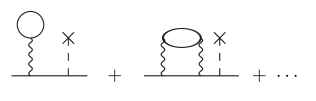
c)

Figure 1: a) Feynman diagrams which enter the single-impurity T-matrix used in our calculation. Bold lines are full (i.e. interacting) propagators $\hat{\mathcal{G}}^{0}$, the cross denotes impurity scattering with strength $\hat{g}_{s}$. b) Sample diagrams contained in a), where thin lines are now non-interacting propagators, and the wavy line represents the interaction $U$. c) An interference process between $\hat{g}_{s}$ and $U$ which is neglected in a).

In our calculations for the interacting system, we shall employ the following approximations: (i) We neglect interference process between different impurities, formally $\hat{T}_{ij}\rightarrow\hat{t}\delta_{ij}$. (ii) We capture the scattering effects using Eqs. (III.2) and (19), i.e., we evaluate a single-impurity T-matrix $\hat{t}$ according to (19) with full (i.e. interacting) propagators $\hat{\mathcal{G}}^{0}$. This neglects processes where impurity scattering and electron-electron interactions interfere, as illustrated in Fig. 1. The change in local density of states induced by the potential scattering can then be expressed as

$$\delta\rho({\bf r},\omega)\equiv\rho({\bf r},\omega)-\rho_{0}({\bf r},\omega)$$ (20)

$$=-\frac{1}{\pi}{\rm Im}\mbox{Tr}\left[\sum_{i}\hat{\mathcal{G}}^{0}({\bf r}-{\bf R}_{i},\omega){\hat{t}}(\omega)\hat{\mathcal{G}}^{0}({\bf R}_{j}-{\bf r},\omega)\right].$$

(iii) Unless otherwise noted, we employ the lowest-order Born approximation, i.e., $\hat{t}=\hat{g}_{s}$.

The approximations (i)–(iii) are designed to capture the effect of weak impurity scattering. They do not account for impurity-induced local changes in the Kondo screening,kaul07 ; morr11 a description of which would require a solution of real-space DMFT equations with a self-consistent set of impurity problemshelmes – a task which we leave for future work.

III.3 Quasiparticle interference

If we Fourier transform $\delta\rho({\bf r},\omega)$ (20) into momentum space and restrict ourselves to the lowest Born approximation, we find

$$\delta\rho({\bf q},\omega)=\frac{-1}{\pi}(\sum_{j}e^{i{\bf q}\cdot{R}_{j}}){\rm Im}\sum_{{\bf k}}\left[\hat{\mathcal{G}}^{0}({\bf k},\omega)\hat{g}_{s}\hat{\mathcal{G}}^{0}({\bf k}+{\bf q},\omega)\right]$$ (21)

i.e, to leading order in the impurity strength, the FT of the LDOS separates into a factor from the QPI of $\hat{\mathcal{G}}^{0}$, describing “band structure”, and another factor representing the spatial distribution of the scatters. The latter is a smooth function of momentum; it is relevant for the overall intensity distribution of $\delta\rho({\bf q},\omega)$ in momentum space, but not for the presence of sharp features (peaks, ripples etc.).

Therefore, we may restrict the calculation to the case of a single impurity, say at ${\bf R_{i}=0}$. We note that this type of approximation (single impurity, T-matrix approximation in the presence of interactions) has been frequently used to describe QPI phenomena in various physical systems in the past (see e.g. Refs. qpi_cup, ; wanglee03, ; qpi_pnic, ; qpi_topo, ). Using (12), the impurity-induced change in differential tunneling conductance, i.e. its spatially inhomogeneous piece, is given

$$\delta\frac{dI}{dV}({\bf r},eV) = -g_{s}\rho_{tip}\frac{2e}{\hbar}\int d\omega\,\,f^{\prime}(\omega-eV)\times$$

$${\rm Im}\left[t_{c}^{2}\mathcal{G}^{0}_{cc}({\bf r},\omega)\mathcal{G}^{0}_{cc}(-{\bf r},\omega)+t_{f}^{2}\mathcal{G}^{0}_{fc}({\bf r},\omega)\mathcal{G}^{0}_{cf}(-{\bf r},\omega)\right.$$

$$+t_{c}t_{f}\mathcal{G}^{0}_{cc}({\bf r},\omega)\mathcal{G}^{0}_{cf}(-{\bf r},\omega)+\left.t_{c}t_{f}\mathcal{G}^{0}_{fc}({\bf r},\omega)\mathcal{G}^{0}_{cc}(-{\bf r},\omega)\right].$$

Note that no $\mathcal{G}^{0}_{ff}$ appears here because of the structure of the scattering potential $\hat{g}_{s}$ (16). Transforming to Fourier space and assuming inversion symmetry, we obtain

$$\delta\frac{dI}{dV}({\bf q},eV)\propto\sum_{{\bf k}} {\rm Im} \left[t_{c}^{2}\,\,\mathcal{G}^{0}_{cc}({\bf k},eV)\mathcal{G}^{0}_{cc}({\bf k}+{\bf q},eV)\right.$$

$$+ \left.t_{f}^{2}\,\,\mathcal{G}^{0}_{fc}({\bf k},eV)\mathcal{G}^{0}_{cf}({\bf k}+{\bf q},eV)\right.$$

$$+ \left.2t_{c}t_{f}\,\,\mathcal{G}^{0}_{cc}({\bf k},eV)\mathcal{G}^{0}_{cf}({\bf k}+{\bf q},eV)\right]$$

which is the equation we will use below to generate numerical results describing QPI. Note that the Fourier-transformed LDOS is complex in general, but the present situation obeys inversion symmetry w.r.t. the position of the single impurity, and hence $dI/dV({\bf q},eV)$ is real.

In general, QPI phenomena as captured, e.g., by equations (20)–(LABEL:eq:QPI), lead to energy-dependent Friedel oscillations in the LDOS, caused by scattering off the impurities. Those oscillations at an energy $\omega$ are primarily determined by the shape of the iso-energy surface at $\omega$ of the underlying band structure, i.e., the oscillation wavevectors ${\bf q}$ are given by approximate nesting wavevectors or by wavevectors which connect points of high DOS in momentum space. (Note that this argument neglects the influence of the real parts of the propagators which enter in Eqs. (21)–(LABEL:eq:QPI) as well.) Thus, the Fourier transform of the LDOS “ripples”qpi_cup observed in SI-STM experiments allows to approximately extract characteristic wavevectors ${\bf q}(\omega)$ of the underlying electronic state. Below we shall show that QPI in heavy-fermion systems is capable of detecting the Fermi-surface reconstruction from high to low temperatures.

IV Energy scales and general considerations

Before diving into numerical results, let us discuss a few general aspects of heavy-fermion physics relevant to SI-STM experiments performed at variable temperature.

Provided that the Anderson model (1) is close to the Kondo limit, i.e., $U,-\epsilon_{f}\gg V^{2}/W$ where $W$ is the half-bandwidth of the $c$ electrons, local moments will form on the $f$ sites upon cooling below a temperature of order $U$. At those high temperatures, conduction electrons will weakly scatter off those local moments, a process which can be described in perturbation theory in the Kondo coupling $J_{\rm K}$ in (2). Upon cooling, the scattering intensity becomes large when $T$ reaches the single-impurity Kondo temperature $T_{\rm K}$ where perturbation theory breaks down.

In the opposite limit of low temperatures (and in the absence of spontaneous symmetry breaking e.g. by magnetism or superconductivity), a heavy Fermi liquid forms away from half-filling. This Fermi liquid is adiabatically connected to the weakly interacting limit of the PAM (1), and perturbation theory in $U$ is at least formally applicable. The Fermi liquid is bounded in temperature from above by a coherence temperature $T_{\rm coh}$ which acts as an effective Fermi energy for the heavy quasiparticles. Typically $T_{\rm coh}<T_{\rm K}$.

In the low-temperature Fermi-liquid regime, Luttinger’s theorem applies, and consequently the Fermi volume is “large”, i.e., given by $\mathcal{V}_{\rm FL}=K_{d}(n_{\rm tot}\,\mbox{mod}2)$, where $n_{\rm tot}=n_{c}+n_{f}$ is the total number of electrons per unit cell and $K_{d}=(2\pi)^{d}/(2v_{0})$ a phase space factor, with $v_{0}$ the unit cell volume and $d$ the spatial dimensionality. In the limit of small $T_{\rm K}$, it also makes sense to consider a Fermi volume for temperatures $T_{\rm K}\ll T\ll W$. Here, the $f$ electrons do not contribute, leading to a “small” Fermi volume with $\mathcal{V}_{s}=K_{d}n_{c}$.

Inelastic scattering between $c$ and $f$ electrons is particularly strong for intermediate temperatures near $T_{\rm coh},T_{\rm K}$. In fact, a common experimental definition of $T_{\rm coh}$ is via the maximum in the resistivity $\rho(T)$. Thus, one expects that the temperature-driven crossover between the small and large Fermi volumes occurs at a temperature of order $T_{\rm coh},T_{\rm K}$.

The physics of the heavy Fermi liquid can be understood, to some degree, in a picture of renormalized bands: Two bands of non-interacting $c$ and $f$ fermions hybridize with a renormalized hybridization $V_{\rm eff}$. This results in two quasiparticle bands with dispersions

$$E_{{\bf k}}^{\pm}=\frac{\epsilon_{{\bf k}}+\tilde{\epsilon}_{f}\pm\sqrt{(\epsilon_{{\bf k}}-\tilde{\epsilon}_{f})^{2}+4V_{\rm eff}^{2}}}{2},$$ (24)

where $\tilde{\epsilon}_{f}$ is the renormalized energy of the $f$-electrons. These bands describe sharp quasiparticles formed as a mixture of $f$ and $c$ degrees of freedom. The renormalized bands, shown schematically in Fig. 2, are separated in energy by a direct (or optical) gap $\Delta_{\rm opt}=2V_{\rm eff}$ at the crossing of the original conduction band and $\tilde{\epsilon}_{f}$, while the bottom of the upper band is separated from the top of the lower band by an indirect gap $\Delta_{g}\propto\sqrt{V_{\rm eff}W}$. $\Delta_{g}$ is typically called hybridization gap.

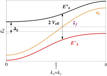
Figure 2: Schematic representation of the $T\rightarrow 0$ band structure expected for a PAM. $V_{\rm eff}$ and $\tilde{\epsilon}_{f}$ are the renormalized hybridization and f-chemical potential respectively. $\Delta_{g}$ is the hybridization gap between the lower and upper renormalized bands.

While this two-band picture is trivially realized at $U=0$ in (1), with $V_{\rm eff}=V$ and $\tilde{\epsilon}_{f}=\epsilon_{f}$, it can be obtained using a slave-boson mean-field approximation from either Eq. (1) in the $U\rightarrow\infty$ limit or from Eq. (2). In both cases, a slave boson $b_{i}$ is introduced such that

$$f^{\dagger}_{i,\sigma}\rightarrow\tilde{f}^{\dagger}_{i,\sigma}b_{i}.$$ (25)

In the simplest approximation, $b$ is uniform and static and measures the effective hybridization between the bands, i.e., $V_{\rm eff}$ in Eq. (24) becomes $V_{\rm eff}=bV$ ($V_{\rm eff}=bJ_{\rm K}$) in the Anderson (Kondo) model. (Note that $b$ is also a measure of the mass renormalization of the quasiparticles, i.e., the mass enhancement is given by $m^{\ast}/m=1/b^{2}$.) This mean-field approximation can be formally justified in a limit where the spin symmetry of the original model is extended from SU(2) to SU($N$) with $N\rightarrow\infty$. Remarkably, the qualitative picture of effective quasiparticle bands, Fig. 2, has been reproduced in numerical treatments of the periodic Anderson (or Kondo lattice) models, using both DMFT grenzebach06 ; assaad_DMFT and its cluster generalizations assaad_CDMFT . Hence, a quasiparticle description of low-temperature heavy-fermion bands appears justified, with a number of caveats noted in the following.

While the slave-boson mean-field theory correctly captures the exponential dependence of the Kondo scale $T_{\rm K}$ on $J_{\rm K}$, $W$, and accounts for the enlargement of the Fermi surface in the Fermi-liquid regime, it misses all inelastic scattering processes, as it only operates with non-interacting fermions. Consequently, the physics not only at finite temperatures, but also that at $T\to 0$ and finite energies is not described well. Both interaction-induced broadening of spectral features away from the Fermi level and incoherent scattering at elevated temperatures are not included. For instance, the hybridization gap in the heavy-fermion state, Fig. 2, is predicted to be a sharp gap in the mean-field theory, but can be expected to be significantly smeared or even washed out by interaction effects. In fact, it has been argued that the experimentally observed Fano-line shape is a consequence of a quasiparticle broadening not captured by the mean-field theory.coleman09 ; woelfle10 More seriously, the crossover from $T\ll T_{\rm K}$ to $T\gg T_{\rm K}$ turns into an artificial phase transition at $T_{\rm K}$ in the slave-boson theory. Hence, to understand the crossover between large and small Fermi volumes upon varying temperature requires at least to treat local correlation effects in a non-perturbative manner – this is what we shall do below using DMFT.

V Numerical results

We have performed extensive studies of the paramagnetic phase of the PAM using DMFT-NRG at various temperatures, tracking the formation of the heavy Fermi liquid upon cooling out of the light conduction band and the $f$-electrons.

For simplicity, we consider a square lattice with nearest-neighbor hopping,

$$\epsilon_{{\bf k}}=-2t(\cos k_{x}+\cos k_{y})+\epsilon_{c}\,,$$ (26)

and half-bandwidth $W=4t$ which we employ as energy unit. We assume the chemical potential to be located at zero energy, such that $\epsilon_{c}$ controls the conduction-band filling.

Most of the figures shown have been obtained with the following set of the PAM parameters: $\epsilon_{c}=0.4$, $\epsilon_{f}=-0.9$, $V=0.55$, $U=10$ (in units of $W$). With these parameters the Anderson width is $\Gamma_{0}\approx 0.51$. In the $T\rightarrow 0$ limit, we find the occupation number of the $c$ ($f$) electrons is $n_{c}\approx 0.57$ ($n_{f}\approx 0.87$), i.e., we work close to the Kondo regime, with a deviation from integer filling comparable to that in actual Ce or Yb heavy-fermion systems. The temperature variation of the band fillings is less than 5% within the temperature range considered here. For the above parameters, we find a $T\to 0$ mass renormalization

$$m^{\ast}/m=\left.1-\frac{\partial{\rm Re}\,\Sigma_{f}(\omega)}{\partial\omega}\right|_{\omega=0}\approx 60$$ (27)

which allows to define a low-temperature Kondo scale $\bar{T}_{\rm K}=\Gamma_{0}\,m/m^{\ast}\approx 8\times 10^{-3}$ – this roughly matches the full width at half maximum (FWHM) of the $T=0$ Abrikosov-Suhl resonance in $\mathcal{G}_{ff}$, see Fig. 5 below. Note, however, that a unique definition of neither the Kondo nor the coherence scale exists, and depending on ones choice may differ by up to an order of magnitude. In our case, we find the temperature scale where the impurity entropy within DMFT reaches $0.5\ln 2$ to be $T_{1/2}\approx 1.5\times 10^{-3}$, and heavy-fermion bands are fully formed only below a coherence temperature of $T_{\rm coh}\approx 2\times 10^{-4}$.

For the 2d system considered here, the van-Hove singularity (vHs) arising from the saddle point in the dispersion is a prominent feature in the DOS which will play a role in all momentum-integrated spectra discussed below.

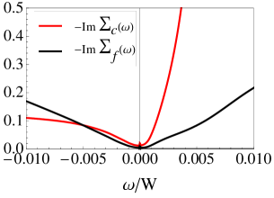
Figure 3: Frequency dependence of the self-energies, ${\rm Im}\Sigma_{f}$ and ${\rm Im}\Sigma_{c}$, of the $f$ and $c$ electrons, respectively, calculated using DMFT-NRG for the periodic Anderson model with parameter $U=10,\epsilon_{f}=-0.9,\epsilon_{c}=0.4,V=0.55$ at a low temperature of $T=1.8\times 10^{-6}$. Energies are given in units of the half-bandwidth $W$.

V.1 Local electronic spectra and self-energies

Once we have solved the self-consistent equation (II.2) for the $f$ self-energy $\Sigma_{f}$, we can form the Green’s function matrix whose elements are given in (6–8). In this section we discuss self-energies as well as the local spectral functions the $c$ and $f$ electrons at different temperatures.

V.1.1 Self-energies

As a check of Fermi-liquid behavior, we start with the frequency dependence of the imaginary parts of the low-temperature electronic self-energies, ${\rm Im}\Sigma_{c}$ and ${\rm Im}\Sigma_{f}$, displayed in Fig. 3. Both exhibit quadratic behavior in $\omega$, in a limited energy range around the Fermi level, as expected for a Fermi liquid. We note that the self-energies have a small residual value at $\omega=0$, arising from both inaccuracies of NRG in fulfilling spectral sum rulesNRGrev and the artificial broadening which has been introduced to stabilize the numerics.grenzebach06 (Our results do not depend on details of this broadening.)

V.1.2 Low-temperature spectra

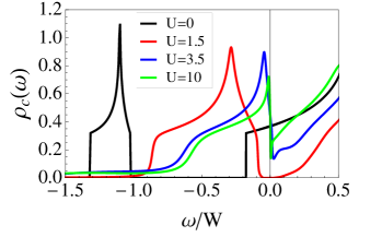
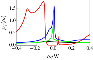
Figure 4: a) $c$ and b) $f$ electron local spectral functions of the periodic Anderson model, calculated using DMFT-NRG at $T=1.8\times 10^{-6}$. The different curves correspond to different values of the local interaction $U$; other parameters are as in Fig. 3. Because the chemical potential is kept fixed, the total and individual band fillings vary as follows: $n_{\rm tot}-n_{c}-n_{f}\approx 2.2-0.42-1.78$ ($U=0$), $1.98-0.78-1.2$ ($U=1.5$), $1.52-0.63-0.89$ ($U=3.5$), and $1.44-0.57-0.87$ ($U=10$).

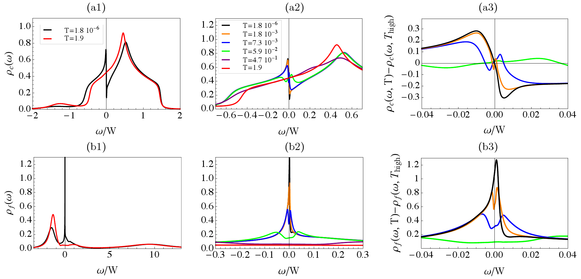
Figure 5: Local spectral functions a) $\rho_{c}(\omega)$ and b) $\rho_{f}(\omega)$ of the PAM calculated using DMFT-NRG for different temperatures $T$, with model parameters as in Fig. 3. a1,b1) Spectra on the full energy range for two temperatures, $T\gg T_{\rm K}$ and $T\ll T_{\rm K}$. a2,b2) Temperature evolution of $\rho_{c}$ and $\rho_{f}$ shown in a restricted energy range near the Fermi level. a3,c3) Low-temperature, low-energy results for $\rho_{c}$ and $\rho_{f}$, with the high-temperature spectra at $T=4.7\times 10^{-1}$ subtracted. The progressive formation of the hybridization pseudogap (panel a) and the Abrikosov-Suhl resonance (panel b) are clearly visible.

Next we turn to the local spectral functions, $\rho_{c}(\omega)=(-1/\pi){\rm Im}\mathcal{G}_{cc}(\omega)$ and $\rho_{f}(\omega)=(-1/\pi){\rm Im}\mathcal{G}_{ff}(\omega)$. To illustrate the effect of interactions and the concomitant deviations from the two-band picture of slave-boson theory explained in Sec. IV, we show the $U$ dependence of the low-temperature spectra in Fig. 4. For the $c$ spectral function, Fig. 4a, increasing $U$ has the following effects: a renormalization of the band positions arising from the real part of the self-energy (note that the chemical potential is kept fixed), a renormalization and simultaneous displacement of the inter-band gap, and its smearing due to the quasiparticle broadening induced by ${\rm Im}\Sigma_{c}(\omega)$. While the two first effects are accounted for in the slave-boson theory, the last is absent in this approximation. The progressive smearing of the hard gap at $U=0$ and its displacement are also visible in the $f$ spectrum, Fig. 4b. Increasing $U$ induces the formation of the Kondo peak (or Abrikosov-Suhl resonance) near the Fermi level. Its width can be considered as a measure of the Kondo scale $T_{\rm K}$, which approaches a finite value in the $U\rightarrow\infty$ limit (due to the finite $\epsilon_{f}$).

A few comments are in order: A sharply defined hybridization gap in $\rho_{c}$, corresponding to the indirect gap $\Delta_{g}$ of Fig. 2, is only present for $U\lesssim 2$, while it is reduced to a dip or pseudogap for larger values of $U\gtrsim 3$. Remarkably, with increasing $U$ one observes an apparent pinning of the vHs of the $c$ band to the Fermi level. As will become clear from the band structures discussed below, this is due to the progressive narrowing of the lower quasiparticle band at low energies. As a result, the vHs and hybridization gap feature cannot be clearly separated in $\rho_{c}$ (both exist on an energy scale of order $T_{\rm K}$). The vHs is also responsible for the strong particle-hole asymmetry of the $c$ spectra. In $\rho_{f}$ both the vHs and the hybridization gap are less prominent. Finally, we remind the reader that our single-orbital PAM does not account for multiple $f$ levels and their crystal-field splitting, i.e., we only model the physics of the lowest-energy crystal-field doublet.

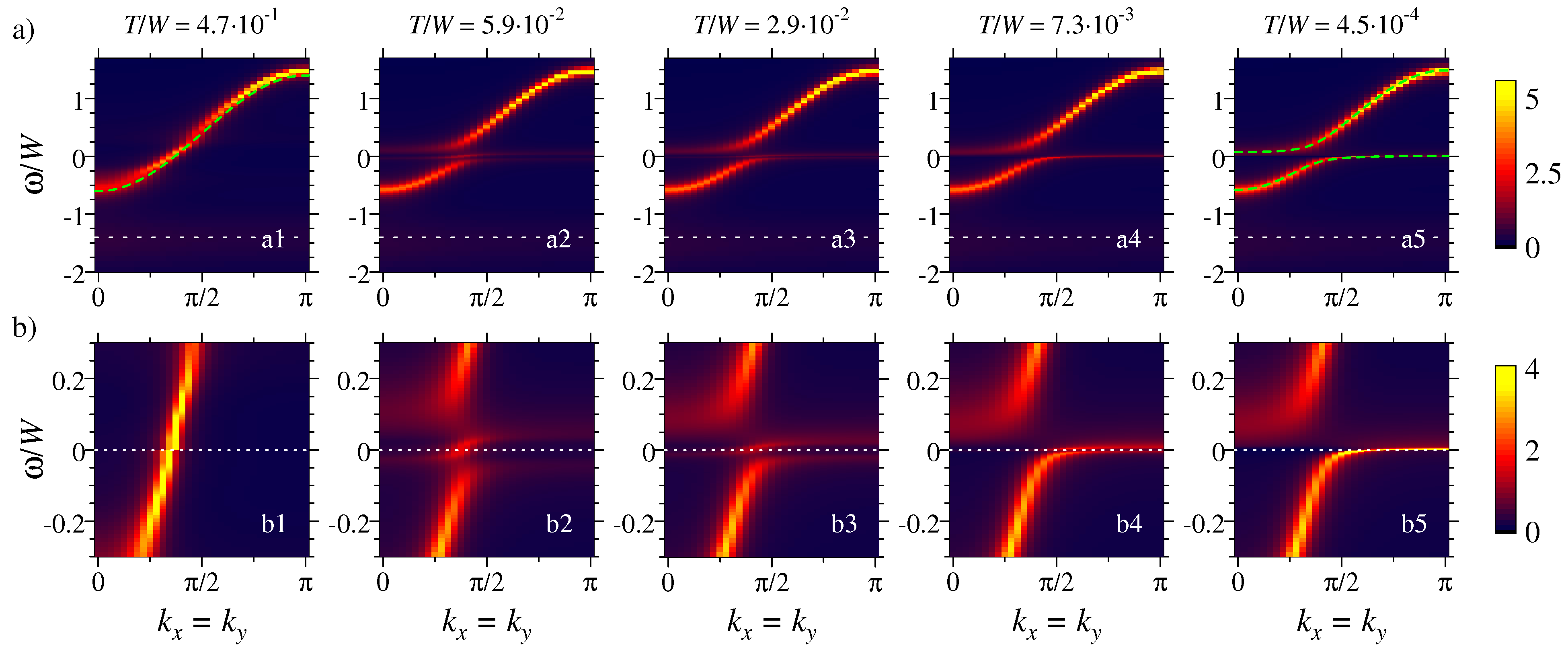
Figure 6: Evolution of the electronic spectrum of the PAM, with parameters as in Fig. 3, with temperature: Shown is $(-1/\pi){\rm Im}(\mathcal{G}_{ff}+\mathcal{G}_{cc})({\bf k},\omega)$ as function of $k_{x}=k_{y}$ and $\omega$ over a) the full range of energies and b) a restricted energy window near the Fermi level. In a) the dotted horizontal lines mark the renormalized $f$ level (i.e. the lower Hubbard band), while in b) the dotted lines represent the Fermi level. Further the dashed line in a1) shows the bare conduction band $\epsilon_{{\bf k}}$. At low temperatures, the formation of heavy bands is obvious, with the reconstruction happening mainly within the optical gap. In a5) the dashed lines represent a fit of the intensity at elevated energies to the effective two-band picture using (24) with $V_{\rm eff}=0.17,\tilde{\epsilon}_{f}=0.025$, and $\tilde{\epsilon}_{c}=0.47$, for detail see text.

V.1.3 Temperature evolution of spectra

The temperature evolution of both $c$ and $f$ local spectral functions in the Kondo regime ($U=10$) is shown in Fig. 5. As can be seen in Fig. 5b1, the $f$ spectrum has the well-known three-peak structure at low temperature: the two charge excitation peaks at $\epsilon_{f}$ and $\epsilon_{f}+U$, well separated from the Abrikosov-Suhl resonance at the Fermi level. The latter is absent at high temperature and is the fingerprint of the Kondo effect. A close-up view of $\rho_{f}(\omega)$ near the Fermi level, Figs. 5b2 and 5b3, shows the development of this resonance with decreasing temperatures.

In the local $c$ spectrum, Fig. 5a1, cooling induces the hybridization pseudogap and a second van-Hove singularity near the Fermi level. This is again shown in detail in Figs. 5a2 and 5a3, where the development of a positive-frequency dip with decreasing temperatures is emphasized. As noted above, this dip is what remains of the hybridization gap once inelastic scattering is fully taken into account; its particle-hole asymmetry is a band-structure effect arising from the low-energy vHs in the present 2d case. The displacement of the higher-energy vHs in Fig. 5a2 can be taken as a measure of ${\rm Re}\Sigma_{c}$. The low-energy structures apparent at intermediate temperature $\approx 10^{-3}\ldots 10^{-2}$ are connected with the dynamical character of the band reconstruction and will be discussed in more detail below.

V.2 Renormalized band structure

After presenting the local (i.e. momentum-integrated) spectral functions, we turn to the full momentum dependence of the spectra. (Recall that in DMFT the interaction-induced self-energies are momentum-independent, but the Green’s functions acquire momentum dependence from the non-interacting bands.) Fig. 6 illustrates the temperature evolution of the electronic spectrum in a false-color plot of $(-1/\pi){\rm Im}(\mathcal{G}_{ff}+\mathcal{G}_{cc})({\bf k},\omega)$ as function of energy $\omega$ and momentum ${\bf k}$ along the line $k_{x}=k_{y}$. At high temperature $T\gg T_{\rm K}$, Fig. 6a1, the signal consists of the rather sharp bare $c$ band and the “atomic” $f$ levels at $\epsilon_{f}$ and $\epsilon_{f}+U$, the latter being broadened by the hybridization. In the opposite limit $T\ll T_{K}$, Fig. 6a5, we have two self-energy-broadened bands, both being rather flat near the Fermi level. One may fit this low-temperature band structure using the two-band picture described in Sec. IV. However, we find that there is no unique fit for all energies: The features at elevated energies are well described by the fit shown in Fig. 6a5, which, however, overestimates the low-energy slope of the heavy band by a factor of 2.5. Alternatively, a low-energy fit results in $V_{\rm eff}=0.072$, consistent with $m^{\ast}/m\approx 60$ obtained from DMFT self-energy – this implies that the DMFT result has to be understood in terms of an energy-dependent band hybridization.

The reconstruction of the band structure from a weakly interacting $c$ band and $f$ levels at high temperature to two heavy bands at low temperature occurs mainly within the optical gap $\sim 2V_{\rm eff}$, as can be seen from Fig. 6b: Portions outside this window show little variation with temperature. When temperature is decreased, spectral weight is transferred gradually from the bare $c$ band near the small Fermi surface to the parts of the incipient heavy-fermion bands near the boundaries of the momentum window. Importantly, for a given energy this weight transfer happens at an energy-dependent temperature, i.e., upon cooling higher energies are reconstructed first, Figs. 6b2–6b4. As a result of this dynamical reconstruction, there is an “island” of spectral intensity near the bare $c$ band left at intermediate temperature, Fig. 6b2, which shrinks and finally disappears upon cooling to significantly lower $T$.

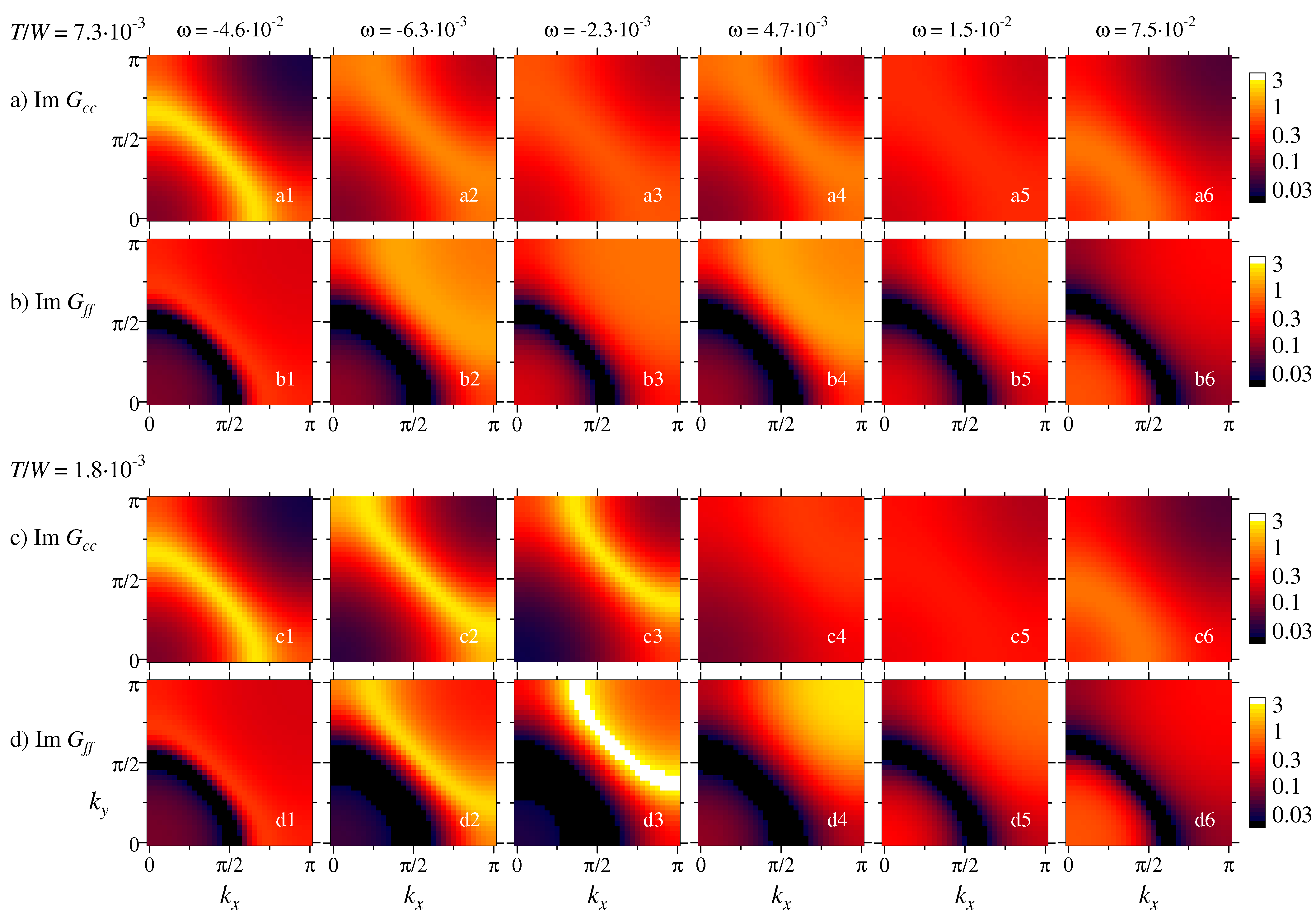
Figure 7: Constant-energy cuts through the electronic spectra of the PAM, with parameters as in Fig. 3. Panels a) and c) show $(-1/\pi){\rm Im}\mathcal{G}_{cc}({\bf k},\omega)$ in a quarter of the first Brillouin zone, panels b) and d) show $(-1/\pi){\rm Im}\mathcal{G}_{ff}({\bf k},\omega)$. The temperatures are a,b) $T=7.3\times 10^{-3}$ and c,d) $T=1.8\times 10^{-3}$. Note that the intensity color scale is logarithmic in all cases.

Constant-energy cuts of the spectral functions, now separated into $(-1/\pi){\rm Im}\mathcal{G}_{ff}$ and $(-1/\pi){\rm Im}\mathcal{G}_{cc}$, illustrating the weight distribution in 2d momentum space, are shown in Fig. 7 for two different temperatures (higher than the one at which the renormalized bands are fully constructed, which is roughly $2\times 10^{-4}$). The plots allow to track in detail the spectral-weight transfer from the high-temperature bare conduction band to the low-temperature renormalized bands; note that we have employed a logarithmic color scale in order to visualized weak-intensity features as well.

Starting the discussion with $c$ electron spectrum, we confirm that there is essentially no temperature dependence for energies outside the optical gap, compare panels a1) and a6) to c1) and c6) in Fig. 7. In contrast, for energies inside the optical gap one observes a significant temperature dependence: At higher temperatures a rather diffuse signal is present in panels a2)–a5), while quasiparticle peaks form at low $T$ and negative energies, panels c2) and c3), and spectral weight disappears at low $T$ and positives energies, panels c4) and c5) – the latter correspond to energies inside the hybridization gap. Note that panel Fig. 7a4 contains shows a well-defined (albeit weak) iso-energy contour – this represents a yet unreconstructed piece of the light band which only disappears at lower temperature, see also Fig. 6b.

The $f$ electron spectra in all panels, Fig. 7b,d, show a pronounced weight reduction which follows closely the “small” Fermi surface defined by $\omega-\epsilon_{\bf k}-{\rm Re}\Sigma_{c}(\omega)=0$; this effect can be easily deduced from Eq. (7) (given that the interaction-induced self-energy has a non-zero imaginary part). A well-defined quasiparticle peak is only visible in $\mathcal{G}_{ff}$ at frequencies where portions of the new renormalized bands are constructed, i.e., in panels d2) and d3).

V.3 Differential tunneling conductance

In the presence of lattice translational symmetry, i.e., in the absence of impurities, the differential tunneling conductance $dI/dV({\bf r}_{i},\omega)$, Eq. (12), is independent of the spatial position (i.e. lattice site) ${\bf r}_{i}$. It is a measure of the local density of states, but depends on the ratio $t_{f}/t_{c}$ of the tunneling amplitudes.

Fig. 8 shows our results for the energy (or bias-voltage) dependence of $dI/dV$ for different values of $t_{f}/t_{c}$ and each for three representative temperatures, $T\gg T_{K}$, $T\sim T_{K}$, and $T\ll T_{K}$. For small values of $t_{f}/t_{c}$, signatures of the hybridization gap are clearly seen, but – as expected – there is never a hard gap near the Fermi level, in contrast to results from slave-boson mean-field theory.coleman09 ; morr10 ; woelfle10 The reason of course are inelastic scattering processes, captured by DMFT but absent in the static mean-field approximation. (Those were added phenomenologically to explain the smearing of the hard gap near the Fermi level and the appearance of the asymmetric peak in experiments.woelfle10 )

For $t_{f}=0$, Fig. 8a, the differential tunneling conductance is proportional to the $c$-electron LDOS. It is almost flat at high temperature while it has a broad peak and a dip at low $T$, resulting from the interplay of the vHs and the hybridization gap. The particle–hole asymmetry is thus inherited from the conduction band. This asymmetry appears opposite to the one observed experimentallydavis_urusi ; yazdani_urusi in URu₂Si₂; in our calculations, such asymmetry would result upon choosing $n_{c}>1$. (Note that the asymmetry in experiment may be influenced by many factors: conduction band dispersions and fillings, relevant crystal field levels of the Kondo ion, and the tunneling paths relevant for STM.)

For $t_{f}/t_{c}\gg 1$, the main contribution to the differential tunneling conductance comes from the $f$-electron LDOS. Accordingly, a large (Kondo) peak is observed in $dI/dV$ near $\omega=0$ and the low-energy particle-hole asymmetry is inverted. This is shown in Fig. 8b.

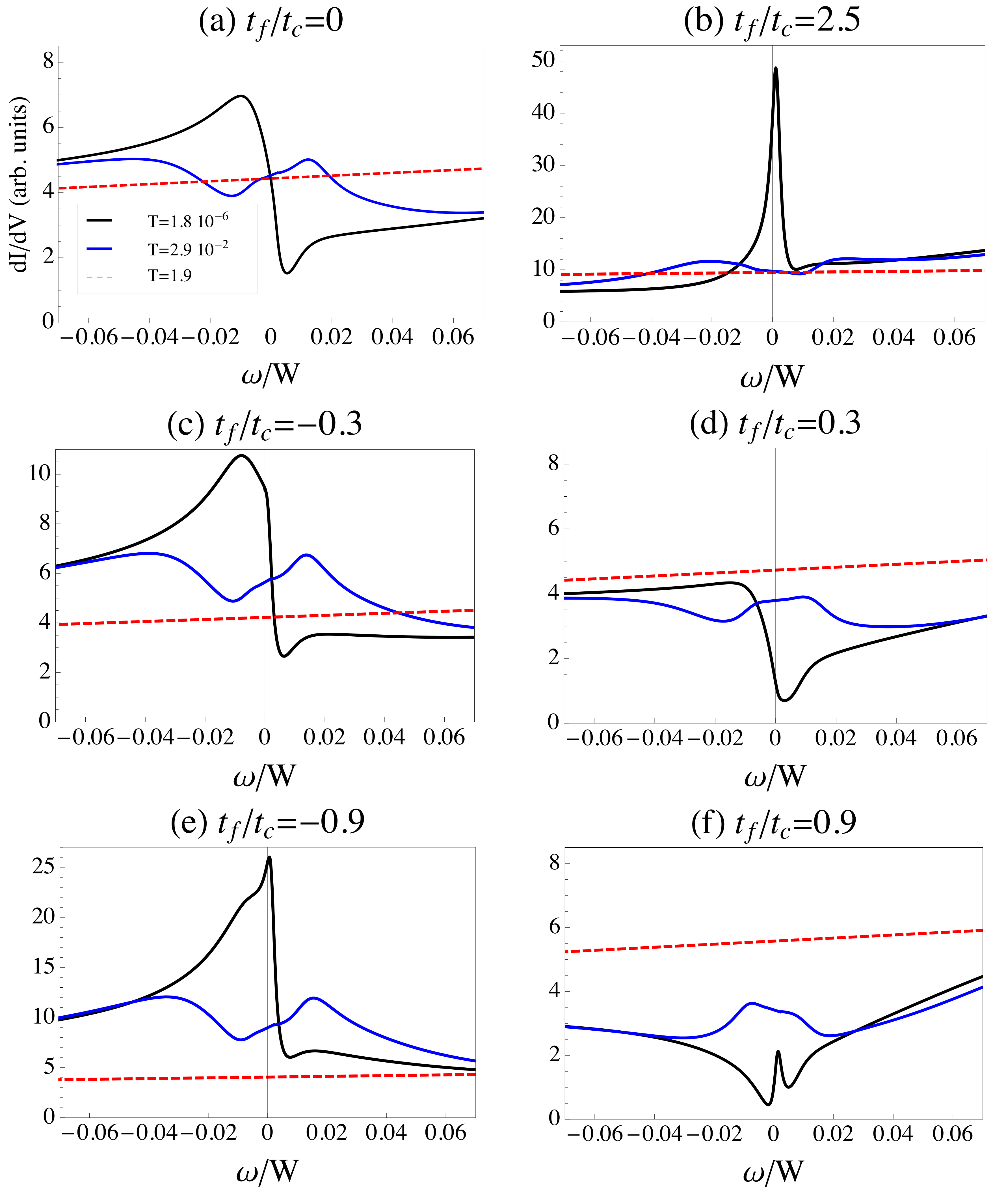
Figure 8: Evolution of the differential conductance $dI/dV$ for small bias voltage with the ratio $t_{f}/t_{c}$ for different temperatures $T\gg T_{K}$, $T\sim T_{K}$ and $T\ll T_{K}$. The effect of destructive [constructive] interference for positive [negative] ratios $t_{f}/t_{c}$ is visible at low temperatures in panels b), d), f) [c) and e)], while the interference is essentially ineffective at high $T$.

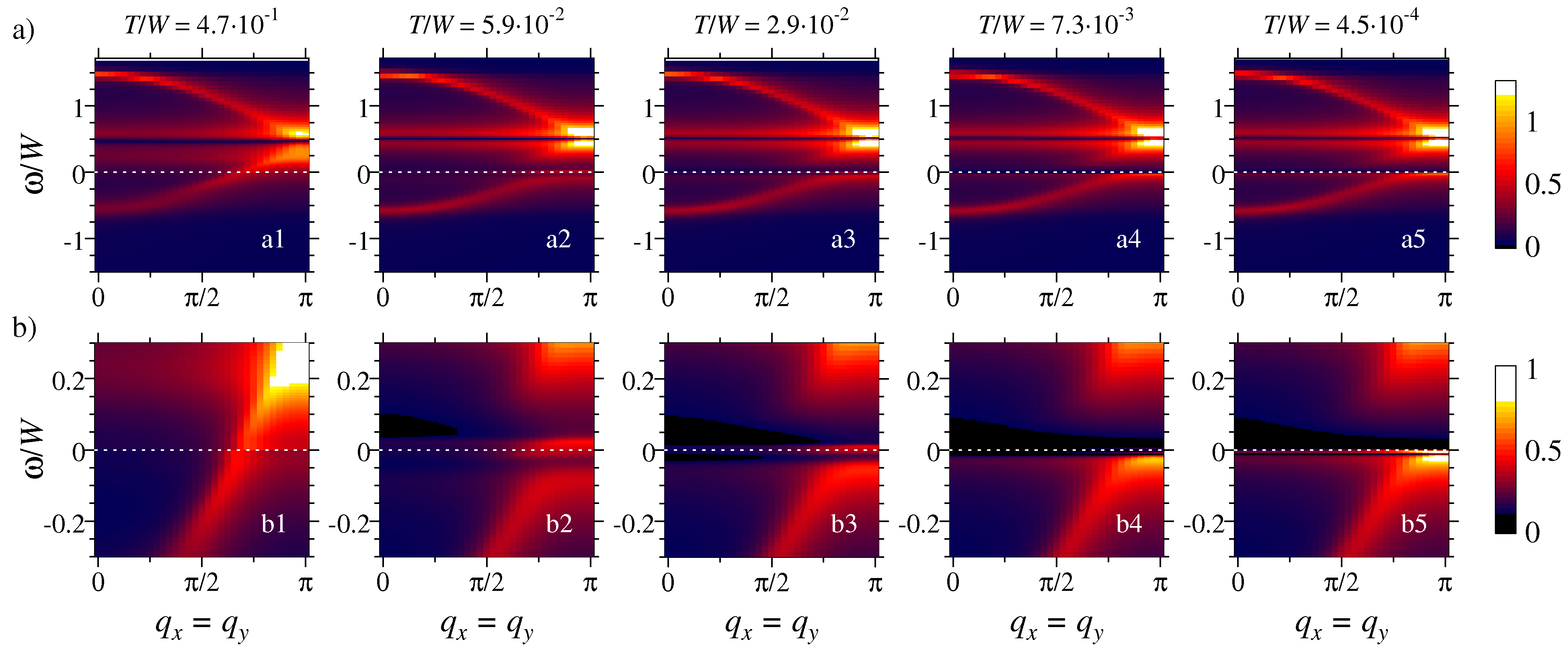
Figure 9: a) Intensity map of the Fourier transform of the spatially inhomogeneous part of the differential tunneling conductance, $|\delta\frac{dI}{dV}({\bf q},\omega)|$, induced by a single point-like weak scalar impurity (i.e. the QPI signal), along the $q_{x}=q_{y}$ direction of the first Brillouin zone. The perculiar behavior near $\omega/W=0.5$ is due to perfect nesting of $\epsilon_{{\bf k}}$, for details see text. b) Close-up near the Fermi level to be compared with the single-electron spectrum in Fig. 6b. The model parameters are as in Fig. 3, the ratio of the tunneling amplitudes is $t_{f}/t_{c}=0$.

For intermediate values of $t_{f}/t_{c}$, quantum interferences between the two tunneling channels have dramatic effects at low temperature as can be seen in Fig. 8c–f. These effects depend on the sign of $t_{f}/t_{c}$. With increasing positive $t_{f}/t_{c}$ and at low temperatures, the vHs peak at negative bias gradually decreases. Then the low-energy particle–hole asymmetry in $dI/dV$ is inverted, Fig. 8d,f, while the Kondo peak emerges near $\omega=0$. Notice that, while the ratio $t_{f}/t_{c}$ increases, the differential tunneling conductance at low $T$ decreases below the one at high temperature before it increases drastically for $t_{f}/t_{c}\gg 1$. The initial decrease is due to destructive interference of the two tunneling channels arising from a negative ${\rm Im}\mathcal{G}_{cf}(\omega)$ (for the $\omega$ range considered here) and positive ratio $t_{f}/t_{c}$. (This effect is essentially ineffective at high temperature.) Conversely, for negative $t_{f}/t_{c}$ we observe constructive interference of the tunneling channels at low $\omega$ and $T$, as can be seen in Fig. 8c,e. Note that the type of interference (constructive vs. destructive) depends on the sign of $t_{f}t_{c}{\rm Im}\mathcal{G}_{cf}(\omega)$, the latter in turn depending on particle-hole asymmetry and microscopic details.

V.4 Quasiparticle interference

Finally, we study quasiparticle-interference phenomena induced by scattering off impurities. As detailed in Sec. III.2, we concentrate on the physics of a single point-like scatterer in the Born limit, which should be appropriate for dilute weak impurities. As is done experimentally, we focus on the intensity in energy-momentum space of the Fourier-transformed differential tunneling conductance, i.e., the magnitude of $|\delta\frac{dI}{dV}({\bf q},E)|$ in Eq. (LABEL:eq:QPI).

V.4.1 QPI and renormalized band structure

We start the discussion of QPI with a plot of $|\delta\frac{dI}{dV}({\bf q},eV)|$ along $q_{x}=q_{y}$ for $t_{f}/t_{c}=0$, Fig. 9, to be compared to the single-particle spectrum shown in Fig. 6.

To understand the QPI result, one has to recall that high QPI intensity at a given energy $\omega$ is expected – within a quasiparticle picture – for wavevectors which connect pieces of the quasiparticle iso-energy contour at $\omega$. Thus, for a simple inversion-symmetric dispersion $\epsilon_{{\bf k}}$, high QPI intensity at $\omega=\epsilon_{{\bf k}}$ will occur for ${\bf q}=2{\bf k}$ such that ${\bf q}$ connects the equal-energy momenta $-{\bf k}$ and ${\bf k}$.

Indeed, by using ${\bf k}={\bf q}/2$ and “unfolding” the plot of $|\delta\frac{dI}{dV}({\bf q},eV)|$ (i.e. adding a mirror image), one can qualitatively recover from Fig. 9 the single-particle spectrum shown in Fig. 6. In particular, the reconstruction of the band structure upon cooling, where spectral weight is transferred within the optical gap near the Fermi level (Sec. V.2), is clearly visible in the QPI plot as well, Fig. 9.

Of course, more complicated band structures, their nesting properties, and the effect of van-Hove singularities are not captured by the above argument. This is nicely visible in our data as well: The QPI signal near the middle of the band is influenced by the nesting properties of the square-lattice dispersion, Eq. (26). The iso-energy contour is a rotated square with perfect nesting in the non-interacting limit. As a result, that QPI response is very strong at ${\bf q}=(\pi,\pi)$, but extends to all wavevectors with $q_{x}=q_{y}$, albeit with a reduced intensity, thanks to the interaction-induced quasiparticle broadening, compare Fig. 9a near $\omega/W\approx 0.5$.

V.4.2 Temperature evolution of QPI

An alternative way to represent QPI data and to discuss its relation to the single-particle spectra is via constant-energy cuts. Such plots are displayed in Figs. 10 and 11, which show the QPI signal together with the $c$ and $f$ spectra for different temperature and energies $\omega=0$ and $\omega=4.7\times 10^{-3}$ (inside the hybridization gap), respectively.

At the Fermi level, Fig. 10, the $c$-electron spectrum illustrates the temperature evolution from the small Fermi surface at high temperature (Fig. 10b1) to the large Fermi surface at low temperature (Fig. 10b5). The $f$-electron spectrum displays a sharp Fermi surface only at low $T$, where the intensity exceeds that in the $c$ spectrum, emphasizing that the low-energy renormalized band has more $f$ than $c$ character.

The QPI signal has a strong intensity at a wave-vector ${\bf q}$ essentially when the $c$ spectrum exhibits a sharp quasiparticle peak at ${\bf q}/2$. In particular, the data at high and low temperature, Figs. 10a1 and 10a5, reflect the corresponding Fermi surfaces. However, a unique extraction of the band structure from QPI may be difficult: Figs. 10a1 and 10a5 look rather similar, due to the fact that the small Fermi surface has an electron volume of $n_{c}\approx 0.6$ while the large Fermi surface has a hole volume $2-n_{c}-n_{f}\approx 0.56$, i.e., both Fermi surfaces yield similar wavevectors for elastic scattering. In actual STM experiments, sub-atomic resolution allows one to obtain information beyond the first Brillouin zone, such that those ambiguities can be partially resolved. At intermediate temperatures $T\sim T_{K}$, the quasiparticle peak in the $c$ spectrum dissolves, and consequently QPI response is very weak and diffuse, Figs. 10a2,a3.

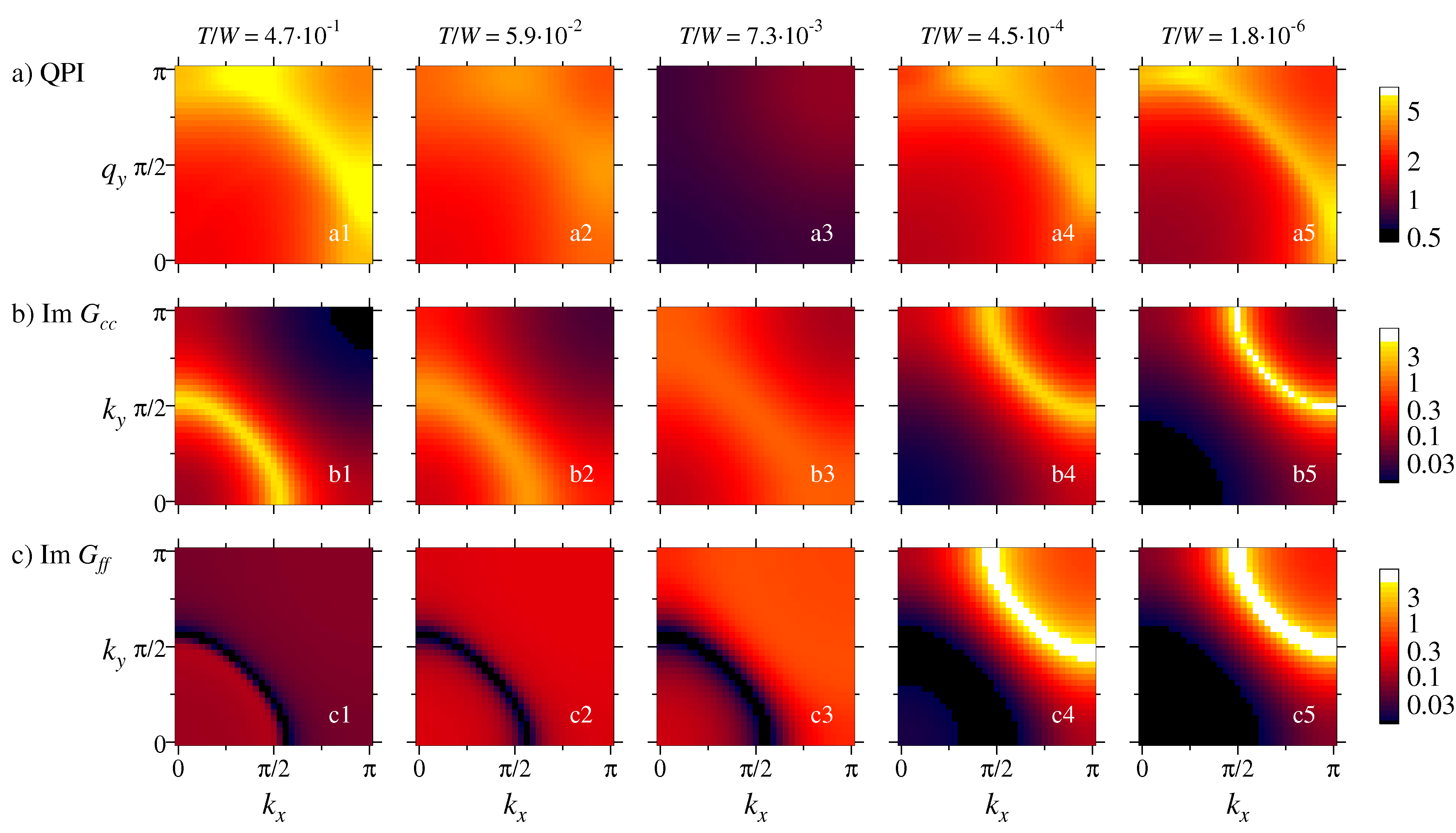
Figure 10: Constant-energy cuts through a) the QPI signal, b) the $c$-electron spectrum, and c) the $f$-electron spectrum, showing a quarter of the first Brillouin zone for different temperatures at an energy $\omega=0$. The ratio of the tunneling amplitudes is $t_{f}/t_{c}=0$. The model parameters are the same as in Fig. 3.

It is instructive to compare the signal at the Fermi level, Fig. 10, to that at an energy inside the hybridization gap, Fig. 11. Again, at high temperature, we have a sharp quasiparticle peak in the $c$ spectrum, corresponding to the band forming a small Fermi surface, and, accordingly, an intense QPI response at the wavevectors connecting portions of this iso-energy contour. Upon lowering the temperature, both the quasiparticle peak and the QPI intensity decrease and essentially disappear completely at the lowest temperature. This nicely reflects the absence of well-defined quasiparticles inside the hybridization gap, i.e., all intensity inside this pseudogap is incoherent.

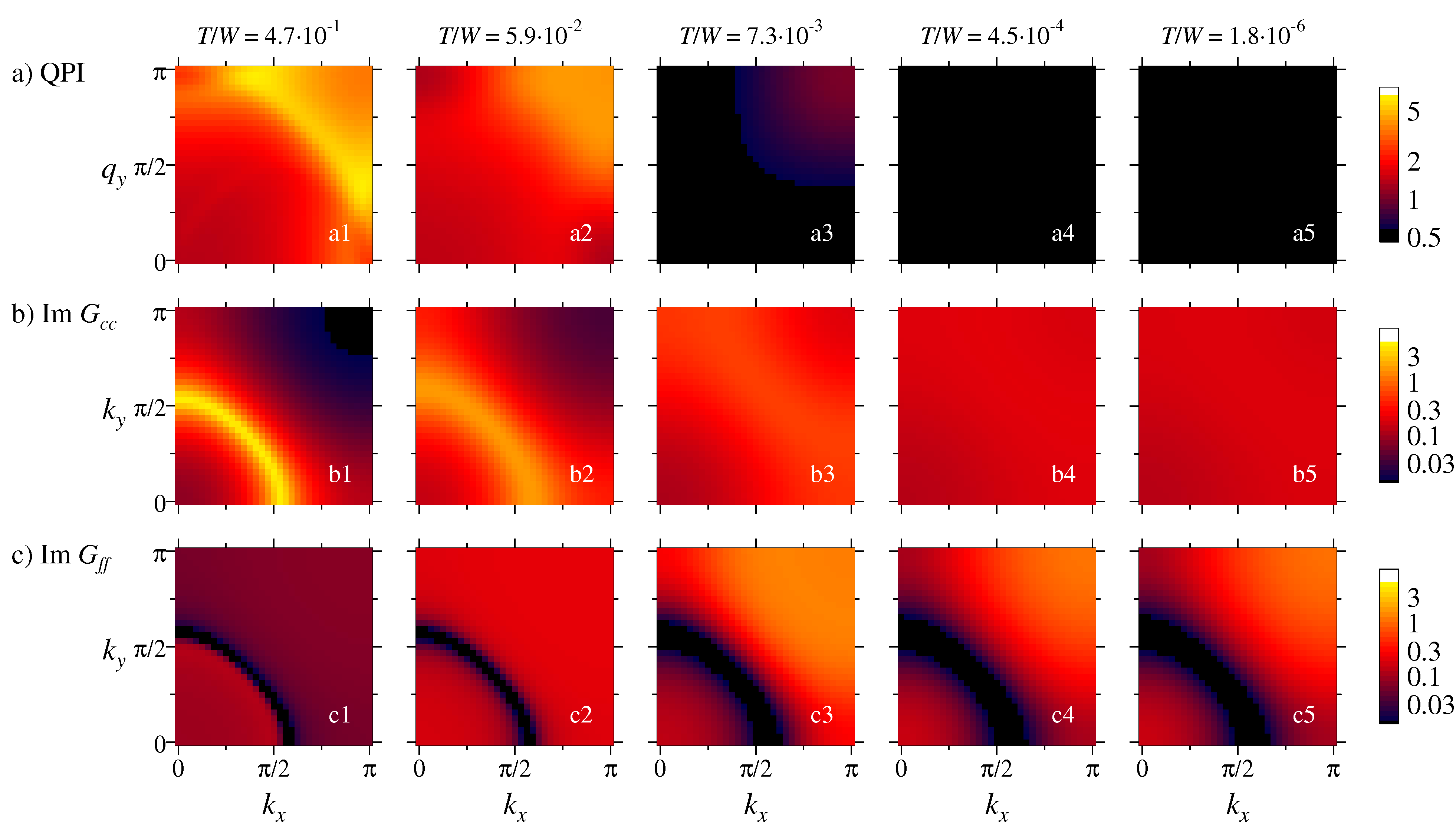
Figure 11: Same as in Fig. 10, but for an energy of $\omega=7.4\times 10^{-3}$ inside the hybridization gap.

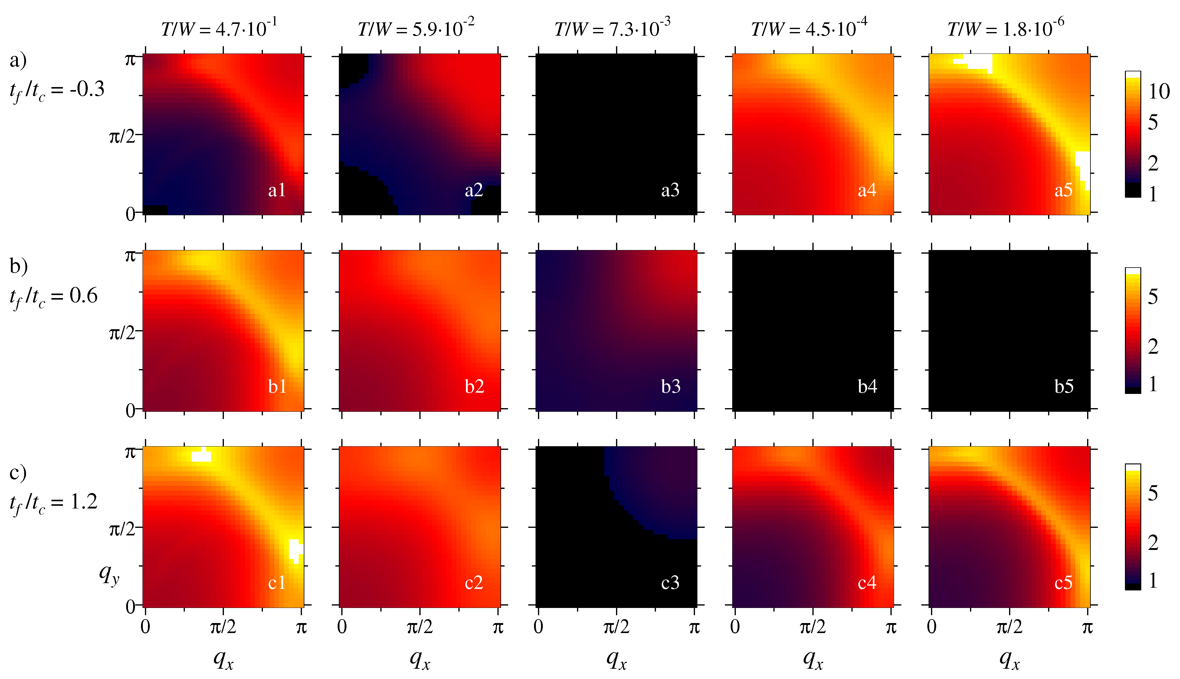
Figure 12: QPI signal at zero bias, $\omega=0$, and different temperatures, now showing the variation with the ratio of the tunneling amplitudes $t_{f}/t_{c}$. a) $t_{f}/t_{c}=-0.3$, b) $t_{f}/t_{c}=0.6$, c) $t_{f}/t_{c}=1.2$. The model parameters are the same as in Fig. 3.

V.4.3 Tunneling paths and QPI

To complete our survey, we show the QPI signal at the Fermi level, $\omega=0$, for a finite ratio of the tunneling amplitudes $t_{f}/t_{c}$ in Fig. 12. As discussed for the differential conductance in the clean system (Sec. V.3), the destructive (constructive) interference between the two tunneling channels for a positive (negative) ratio $t_{f}/t_{c}$ is apparent through a reduction (enhancement) in the QPI signal at low temperatures, while it is mainly unchanged at high temperature. The effect of the destructive interference can be so strong that it essentially suppresses the QPI signal at low energies and temperatures, as can be seen for $t_{f}/t_{c}=0.6$ in Fig. 12b.

VI Summary

We have analyzed the temperature-dependent electronic spectra in the periodic Anderson model, a paradigmatic model for heavy-fermion formation, using dynamical mean field theory (DMFT) with Wilson’s numerical renormalization group (NRG). Particular attention has been paid to the temperature evolution of the low-energy spectra and the crossover from a ‘”small” Fermi surface of conduction electrons to a ”large” Fermi surface of composite heavy quasiparticles upon cooling. To make contact with STM experiments, we have further studied the differential tunneling conductance, related to local spectral properties of the model, and its modulations arising from impurity scattering processes via quasiparticle interference (QPI). In particular, we go beyond the limitations of previous analytical approaches, based on a slave boson mean-field theory, by fully accounting for interaction-induced broadening of spectral features away from the Fermi level and incoherent scattering processes at elevated temperature.

For the clean system, the local differential tunneling conductance is shown to display an asymmetric peak, similar to the one observed experimentally, whose shape and intensity, apart from material specific details, depend on the ratio of the tunneling amplitudes $t_{c}$ and $t_{f}$ into conduction-electron and $f$-electron states, respectively. (Previous theoretical studies found a hard gap near the Fermi level and recovered the experimentally observed peak only by an ad hoc addition of a phenomenological quasiparticle broadening.) For positive ratio $t_{f}/t_{c}$, the effect of destructive interferences between the two tunneling channels shows itself as a decrease of the differential tunneling conductance intensity at low temperature, while it is mainly inefficient at high temperature.

By studying at the momentum-dependent spectral functions at different temperatures, we unveiled the dynamical reconstruction of the Fermi surface which happens mainly within the optical gap. In this window of energies, spectral weight at high frequencies is transferred from the bare conduction band to the edges of the renormalized bands when the temperature is lowered down to zero. Islets of spectral weight at the Fermi level persist but become smaller and smaller with decreasing temperatures until merging completely with the incipient band structure in the $T\rightarrow 0$ limit. This underlines the energy dependence of the crossover from a “small” to a “large” Fermi surface: this crossover, characterized by dissolving quasiparticle peaks, happens at a frequency-dependent temperature.

Quasiparticle interference induced by impurity scatterers offers an opportunity to follow such a dynamical reconstruction, as one can at least partially reconstruct the band structure from the dispersive high-intensity features of the QPI response. However, we have also shown that this may be seriously hindered by the destructive effect of the interference between the two tunneling channels (here for positive ratio $t_{f}/t_{c}$), which may lead to an almost complete extinction of QPI for certain energies.

Our detailed study spans many issues that are of relevance for existing and forthcoming spectroscopic measurements on heavy-fermion materials. It would be particularly interesting to study the energy-dependent crossover between small and large Fermi surfaces advocated here. Layered heavy-fermion materials, e.g. of the so-called 115 family (CeCoIn₅ and relatives) are most promising in this context, and corresponding experiments are underway.yaz11

- (1) A. C. Hewson, The Kondo Problem to Heavy Fermions, Cambridge University Press, Cambridge (1997).
- (2) P. Coleman, in: Handbook of Magnetism and Advanced Magnetic Materials (eds H. Kronmüller and S. Parkin), vol. 1, p. 45, Wileys, New York (2007).
- (3) G. R. Stewart, Rev. Mod. Phys. 73, 797 (2001).
- (4) H. v. Löhneysen, A. Rosch, M. Vojta, and P. Wölfle, Rev. Mod. Phys. 79, 1015 (2007).
- (5) J. Lee, M. P. Allan, M. A. Wang, J. Farrell, S. A. Grigera, F. Baumberger, J. C. Davis, and A. P. Mackenzie, Nature Phys. 5, 800 (2009).
- (6) A. R. Schmidt, M. H. Hamidian, P. Wahl, F. Meier, A. V. Baltsky, J. D. Garrett, T. J. Wiliams, G. M. Luke, and J. C. Davis, Nature 465, 570 (2010).
- (7) P. Aynajian, E. H. Da Silva Neto, C. V. Parker, Y. Huang, A. Pasupathy, J. Mydosh, and A. Yazdani, PNAS 107, 10383 (2010).
- (8) S. Ernst, S. Kirchner, C. Krellner, C. Geibel, G. Zwicknagl, F. Steglich, and S. Wirth, Nature 474, 362 (2011).
- (9) M. F. Crommie, C. P. Lutz, and D. M. Eigler, Nature 363, 524 (1993).
- (10) J. E. Hoffman, K. McElroy, D.-H. Lee, K. M Lang, H. Eisaki, S. Uchida, and J. C. Davis, Science 297, 1148 (2002).
- (11) K. McElroy, R. W. Simmonds, J. E. Hoffman, D.-H. Lee, J. Orenstein, H. Eisaki, S. Uchida, and J. C. Davis, Nature 422, 592 (2003).
- (12) L. Capriotti, D. J. Scalapino, and R. D. Sedgewick, Phys. Rev. B 68, 014508 (2003).
- (13) Q. H. Wang and D. H. Lee, Phys. Rev. B 67, 020511 (2003).
- (14) M. Maltseva, M. Dzero, and P. Coleman, Phys. Rev. Lett. 103, 206402 (2009).
- (15) J. Figgins and D. K. Morr, Phys. Rev. Lett. 104, 187202 (2010).
- (16) P. Wölfle, Y. Dubi, and A. V. Balatsky, Phys. Rev. Lett. 105, 246401 (2010).
- (17) W. Metzner and D. Vollhardt, Phys. Rev. Lett. 62, 324 (1989).
- (18) A. Georges, G. Kotliar, W. Krauth, and M. J. Rozenberg, Rev. Mod. Phys. 68, 13 (1996).
- (19) R. Bulla, T. A. Costi, and T. Pruschke, Rev. Mod. Phys. 80, 395 (2008).
- (20) O. Sakai and Y. Kuramoto, Solid State Commun. 89, 307 (1994)
- (21) R. Bulla, Phys. Rev. Lett. 83, 136 (1999).
- (22) R. Bulla, T. A. Costi, and D. Vollhardt, Phys. Rev. B 64, 045103 (2001)
- (23) T. Pruschke, R. Bulla, and M. Jarrell, Phys. Rev. B 61, 12799 (2000).
- (24) Y. Shimizu, O. Sakai, and A. C. Hewson, J. Phys. Soc. Jpn. 69, 1777 (2000).
- (25) R. Bulla, A. C. Hewson, and T. Pruschke, J. Phys.: Condens. Matter 10, 8365 (1998).
- (26) T. A. Costi and N. Manini, J. Low Temp. Phys. 126, 835 (2002).
- (27) C. Grenzebach, F. B. Anders, G. Czycholl, and T. Pruschke, Phys. Rev. B 74, 195119 (2006).
- (28) C. Grenzebach, F. B. Anders, G. Czycholl, and T. Pruschke, Phys. Rev. B 77, 115125 (2008).
- (29) O. Bodensiek, R. Zitko, R. Peters, and T. Pruschke, J. Phys.: Condens. Matter 23, 094212 (2011).
- (30) V. Madhavan, W. Chen, T. Jamneala, M. F. Crommie, and N. S. Wingreen, Science 280, 567 (1998).
- (31) O. Újsághy, J. Kroha, L. Szunyogh, and A. Zawadowski, Phys. Rev. Lett. 85, 2557 (2000).
- (32) Strictly speaking, the tunneling of electrons from the tip to the system is a non-equilibrium process. However, the amplitude of the current in STM experiments is sufficiently small that the time between two tunneling events is much longer than the typical electronic relaxation time. Then the thermal equilibrium assumption is appropriate.
- (33) R. K. Kaul and M. Vojta, Phys. Rev. B 75, 132407 (2007).
- (34) J. Figgins and D. K. Morr, Phys. Rev. Lett. 107, 066401 (2011).
- (35) R. W. Helmes, T. A. Costi, and A. Rosch Phys. Rev. Lett. 100, 056403 (2008).
- (36) Y.-Y. Zhang, C. Fang, X. Zhou, K. Seo, W.-F. Tsai, B. A. Bernevig, and J. Hu, Phys. Rev. B 80, 094528 (2009).
- (37) H.-M. Guo and M. Franz, Phys. Rev. B 81, 041102 (2010).
- (38) K. S. D. Beach and F. F. Assaad, Phys. Rev. B 77, 205123 (2008).
- (39) L. C. Martin and F. F. Assaad, Phys. Rev. Lett. 101, 066404 (2008); L. C. Martin, M. Bercx, and F. F. Assaad, Phys. Rev. B 82, 245105 (2010).
- (40) P. Aynajian, A. Yazdani et al., unpublished.