Nonconvex proximal-splitting: batch and incremental algorithms

Abstract

We study a class of large-scale, nonsmooth, and nonconvex optimization problems. In particular, we focus on nonconvex problems with composite objectives. This class includes the extensively studied convex, composite objective problems as a subclass. To solve composite nonconvex problems we introduce a powerful new framework based on asymptotically nonvanishing errors, avoiding the common stronger assumption of vanishing errors. Within our new framework we derive both batch and incremental proximal splitting algorithms. To our knowledge, our work is first to develop and analyze incremental nonconvex proximal-splitting algorithms, even if we were to disregard the ability to handle nonvanishing errors. We illustrate one instance of our general framework by showing an application to large-scale nonsmooth matrix factorization.

1 Introduction

This paper focuses on nonconvex composite objective problems having the form

$$\text{minimize}\quad\Phi(x):=f(x)+h(x)\qquad x\in\mathcal{X},$$ (1)

where $f:\mathbb{R}^{n}\to\mathbb{R}$ is continuously differentiable and possibly nonconvex, $h:\mathbb{R}^{m}\to\mathbb{R}\cup\left\{{\infty}\right\}$ is lower semi-continuous (lsc) and convex (possibly nonsmooth), and $\mathcal{X}$ is a compact convex set. We also make the common assumption that $f$ has a Lipschitz continuous gradient within $\mathcal{X}$, written as $f\in C_{L}^{1}(\mathcal{X})$; that is, there is a constant $L>0$ such that

$$\|{\nabla f(x)-\nabla f(y)}\|\leq L\|{x-y}\|\qquad\text{for all}\quad x,y\in\mathcal{X}.$$ (2)

Problem (1) is a natural but far-reaching generalization of composite objective convex problems, which continue to enjoy tremendous importance in machine learning; see e.g., [Duchi and Singer 2009, Bach et al. 2011, Xiao 2009, Beck and Teboulle 2009]. Although, convex formulations are extremely useful, for many difficult problems a nonconvex formulation is more natural. Familiar examples include matrix factorization [Mairal et al. 2010, Lee and Seung 2000], blind deconvolution [Kundur and Hatzinakos 1996], dictionary learning [Kreutz-Delgado et al. 2003, Mairal et al. 2010], and neural networks [Bertsekas 1999, Haykin 1994].

The primary contribution of this paper is theoretical and algorithmic. Specifically, we present a new framework: Nonconvex Inexact Proximal Splitting (NIPS). Our framework solves (1) by “splitting” the task into smooth (gradient) and nonsmooth (proximal) parts. Beyond splitting, the most notable feature of NIPS is that it allows computational errors. This capability proves critical to obtaining a scalable, incremental-gradient variant of NIPS, which, to our knowledge, is the first incremental nonconvex proximal-splitting method in the literature.

A further distinction of NIPS lies in how it models computational errors. Notably, NIPS does not require the errors to vanish in the limit, a realistic assumption as often one has limited to no control over computational errors inherent to a complex system. In accord with the errors, NIPS also does not require stepsizes (learning rates) to shrink to zero. In contrast, most incremental-gradient methods [Bertsekas 2010] and stochastic gradient algorithms [Gaivoronski 1994] do assume that the computational errors and stepsizes decay to zero. We do not make these simplifying assumptions, which complicates the convergence analysis but results perhaps in a more satisfying description.

Our analysis builds on the remarkable work of Solodov [1997], who studied the simpler setting of differentiable nonconvex problems (corresponding to the choice $h\equiv 0$ in (1)). NIPS is strictly more general: unlike [Solodov 1997] it solves a non-differentiable problem by allowing a nonsmooth regularizer $h\not\equiv 0$, which it tackles by invoking the fruitful idea of proximal-splitting [Combettes and Pesquet 2010].

Proximal splitting has proved to be exceptionally effective and practical [Combettes and Pesquet 2010, Beck and Teboulle 2009, Bach et al. 2011, Duchi and Singer 2009]. It retains the simplicity of gradient-projection while handling the nonsmooth regularizer $h$ via its proximity operator. This style is especially attractive because for several important choices of $h$, efficient implementations of the associated proximity operators exist [Bach et al. 2011, Liu and Ye 2009, Mairal et al. 2010]. For convex problems, an alternative to proximal splitting is the subgradient method; similarly, for nonconvex problems one could use a generalized subgradient method [Clarke 1983, Ermoliev and Norkin 1998]. However, as in the convex case, the use of subgradients has drawbacks: it fails to exploit the composite structure, and even when using sparsity promoting regularizers it does not generate intermediate sparse iterates [Duchi and Singer 2009].

Among batch nonconvex splitting methods, an early paper is [Fukushima and Mine 1981]. More recently, in his pioneering paper on convex composite minimization, Nesterov [2007] also briefly discussed nonconvex problems. Both [Fukushima and Mine 1981] and [Nesterov 2007], however, enforced monotonic descent in the objective value to ensure convergence. Very recently, Attouch et al. [2011] have introduced a generic method for nonconvex nonsmooth problems based on Kurdyka-Łojasiewicz theory, but their entire framework too hinges on descent.

This insistence on descent makes these methods unsuitable for incremental, stochastic, or online variants, all of which usually lead to a nonmonotone sequence of objective values. Among nonmonotonic methods that apply to (1), we are aware of the generalized gradient-type algorithms of [Solodov and Zavriev 1998] and the stochastic generalized gradient methods of [Ermoliev and Norkin 1998]. Both methods, however, are analogous to the usual subgradient-based algorithms, and fail to exploit the composite objective structure.

But despite its desirability and potential benefits, proximal-splitting for exploiting composite objectives does not apply out-of-the-box to (1): nonconvexity raises significant obstructions, especially because nonmonotonic descent in the objective function values is allowed. Overcoming these obstructions to achieve a scalable non-descent based method is what makes the NIPS framework novel.

2 The NIPS Framework

To simplify presentation, we replace $h$ by the penalty function

$$g(x):=h(x)+\delta({x}|{\mathcal{X}}),$$ (3)

where $\delta({\cdot}|{\mathcal{X}})$ is the indicator function for $\mathcal{X}$: $\delta({x}|{\mathcal{X}})=0$ for $x\in\mathcal{X}$, and $\delta({x}|{\mathcal{X}})=\infty$ for $x\not\in\mathcal{X}$. With this notation, we may rewrite (1) as the unconstrained problem:

$$\min\nolimits_{x\in\mathbb{R}^{n}}\quad\Phi(x):=f(x)+g(x),$$ (4)

and this particular formulation is our primary focus. We solve (4) via a proximal-splitting approach, so let us begin by defining our most important component.

Definition 1 (Proximity operator).

Let $g:\mathbb{R}^{n}\to\mathbb{R}$ be an lsc, convex function. The proximity operator for $g$, indexed by $\eta>0$, is the nonlinear map [see e.g., Rockafellar and Wets 1998; Def. 1.22]:

$$\mathscr{P}_{\eta}^{g}\ :\quad y\mapsto\ \operatorname*{argmin}_{x\in\mathbb{R}^{n}}\ \bigl{(}g(x)+\tfrac{1}{2\eta}\|{x-y}\|^{2}\bigr{)}.$$ (5)

The operator (5) was introduced by Moreau [1962] (1962) as a generalization of orthogonal projections. It is also key to Rockafellar’s classic proximal point algorithm [Rockafellar 1976], and it arises in a host of proximal-splitting methods [Combettes and Pesquet 2010, Duchi and Singer 2009, Bach et al. 2011, Beck and Teboulle 2009], most notably in forward-backward splitting (FBS) [Combettes and Pesquet 2010].

FBS is particularly attractive because of its simplicity and algorithmic structure. It minimizes convex composite objective functions by alternating between “forward” (gradient) steps and “backward” (proximal) steps. Formally, suppose $f$ in (4) is convex; for such $f$, FBS performs the iteration

$$x^{k+1}=\mathscr{P}_{\eta_{k}}^{g}(x^{k}-\eta_{k}\nabla f(x^{k})),\quad k=0,1,\ldots,$$ (6)

where $\left\{{\eta_{k}}\right\}$ is a suitable sequence of stepsizes. The usual convergence analysis of FBS is intimately tied to convexity of $f$. Therefore, to tackle nonconvex $f$ we must take a different approach. As previously mentioned, such approaches were considered by Fukushima and Mine [1981] and Nesterov [2007], but both proved convergence by enforcing monotonic descent.

This insistence on descent severely impedes scalability. Thus, the key challenge is: how to retain the algorithmic simplicity of FBS and allow nonconvex losses, without sacrificing scalability?

We address this challenge by introducing the following inexact proximal-splitting iteration:

$$x^{k+1}=\mathscr{P}_{\eta_{k}}^{g}(x^{k}-\eta_{k}\nabla f(x^{k})+\eta_{k}e(x^{k})),\quad k=0,1,\ldots,$$ (7)

where $e(x^{k})$ models the computational errors in computing the gradient $\nabla f(x^{k})$. We also assume that for $\eta>0$ smaller than some stepsize $\bar{\eta}$, the computational error is uniformly bounded, that is,

$$\eta\|{e(x)}\|\leq\bar{\epsilon},\quad\text{for some fixed error level }\ \bar{\epsilon}\geq 0,\quad\text{and }\forall x\in\mathcal{X}.$$ (8)

Condition (8) is weaker than the typical vanishing error requirements

$$\sum\nolimits_{k}\eta\|{e(x^{k})}\|<\infty,\qquad\lim_{k\to\infty}\eta\|{e(x^{k})}\|=0,$$

which are stipulated by most analyses of methods with gradient errors [Bertsekas 1999; 2010]. Obviously, since errors are nonvanishing, exact stationarity cannot be guaranteed. We will, however, show that the iterates produced by (7) do progress towards reasonable inexact stationary points. We note in passing that even if we assume the simpler case of vanishing errors, NIPS is still the first nonconvex proximal-splitting framework that does not insist on monotonicity, which which complicates convergence analysis but ultimately proves crucial to scalability.

Operator $\mathscr{P}_{\eta}^{g}$, and a sequence $\left\{{\eta_{k}}\right\}$ satisfying

$$c\leq\liminf\nolimits_{k}\eta_{k},\quad\limsup\nolimits_{k}\eta_{k}\leq\min\left\{{1,2/L-c}\right\},\quad 0<c<1/L.$$ (9)

Approximate solution to (7)  

$k\leftarrow 0$; Select arbitrary $x^{0}\in\mathcal{X}$

while $\neg$ converged do

    Compute approximate gradient $\widetilde{\nabla}f(x^{k}):=\nabla f(x^{k})-e(x^{k})$

    Update: $x^{k+1}=\mathscr{P}_{\eta_{k}}^{g}(x^{k}-\eta_{k}\widetilde{\nabla}f(x^{k}))$

    $k\leftarrow k+1$

end while

Algorithm 1 Inexact Nonconvex Proximal Splitting (NIPS)

2.1 Convergence analysis

We begin by characterizing inexact stationarity. A point $x^{*}$ is a stationary point for (4) if and only if it satisfies the inclusion

$$0\in\partial_{C}\Phi(x^{*}):=\nabla f(x^{*})+\partial g(x^{*}),$$ (10)

where $\partial_{C}\phi$ denotes the Clarke subdifferential [Clarke 1983]. A brief exercise shows that this inclusion may be equivalently recast as the fixed-point equation (which augurs the idea of proximal-splitting)

$$x^{*}=\mathscr{P}_{\eta}^{g}(x^{*}-\eta\nabla f(x^{*})),\quad\text{for }\eta>0.$$ (11)

This equation helps us define a measure of inexact stationarity: the proximal residual

$$\rho(x):=x-\mathscr{P}_{1}^{g}(x-\nabla f(x)).$$ (12)

Note that for an exact stationary point $x^{*}$ the residual norm $\|{\rho(x^{*})}\|=0$. Thus, we call a point $x$ to be $\epsilon$-stationary if for a prescribed error level $\epsilon(x)$, the corresponding residual norm satisfies

$$\|{\rho(x)}\|\leq\epsilon(x).$$ (13)

Assuming the error-level $\epsilon(x)$ (say if $\bar{\epsilon}=\lim\sup_{k}\epsilon(x^{k})$) satisfies the bound (8), we prove below that the iterates $\left\{{x^{k}}\right\}$ generated by (7) satisfy an approximate stationarity condition of the form (13), by allowing the stepsize $\eta$ to become correspondingly small (but strictly bounded away from zero).

We start by recalling two basic facts, stated without proof as they are standard knowledge.

Lemma 2 (Lipschitz-descent [see e.g., Nesterov 2004; Lemma 2.1.3]).

Let $f\in C_{L}^{1}(\mathcal{X})$. Then,

$$|f(x)-f(y)-\langle{\nabla f(y)},\,{x-y}\rangle|\leq\tfrac{L}{2}\|{x-y}\|^{2},\quad\forall\ x,y\in\mathcal{X}.$$ (14)

Lemma 3 (Nonexpansivity [see e.g., Combettes and Wajs 2005; Lemma 2.4]).

The operator $\mathscr{P}_{\eta}^{g}$ is nonexpansive, that is,

$$\|{\mathscr{P}_{\eta}^{g}(x)-\mathscr{P}_{\eta}^{g}(y)}\|\leq\|{x-y}\|,\quad\forall\ x,y\in\mathbb{R}^{n}.$$ (15)

Next we prove a crucial monotonicity property that actually subsumes similar results for projection operators derived by Gafni and Bertsekas [1984; Lem. 1], and may therefore be of independent interest.

Lemma 4 (Prox-Monotonicity).

Let $y,z\in\mathbb{R}^{n}$, and $\eta>0$. Define the functions

$$p_{g}(\eta)\quad:=\quad\tfrac{1}{\eta}\|{\mathscr{P}_{\eta}^{g}(y-\eta z)-y}\|,\quad\text{and}\quad q_{g}(\eta)\quad:=\quad\|{\mathscr{P}_{\eta}^{g}(y-\eta z)-y}\|.$$ (16)

Then, $p_{g}(\eta)$ is a decreasing function of $\eta$, and $q_{g}(\eta)$ an increasing function of $\eta$.

Proof.

Our proof exploits properties of Moreau-envelopes [Rockafellar and Wets 1998; pp. 19,52], and we present it in the language of proximity operators. Consider the “deflected” proximal objective

$$m_{g}(x,\eta;y,z):=\langle{z},\,{x-y}\rangle+\tfrac{1}{2\eta}\|{x-y}\|^{2}+g(x),\quad\text{for some}\ y,z\in\mathcal{X}.$$ (17)

Associate to objective $m_{g}$ the deflected Moreau-envelope

$$E_{g}(\eta):=\inf_{x\in\mathcal{X}}\ m_{g}(x,\eta;y,z),$$ (18)

whose infimum is attained at the unique point $\mathscr{P}_{\eta}^{g}(y-\eta z)$. Thus, $E_{g}(\eta)$ is differentiable, and its derivative is given by $E_{g}^{\prime}(\eta)=-\tfrac{1}{2\eta^{2}}\|{\mathscr{P}_{\eta}^{g}(y-\eta z)-y}\|^{2}=-\tfrac{1}{2}p(\eta)^{2}$. Since $E_{g}$ is convex in $\eta$, $E_{g}^{\prime}$ is increasing ([Rockafellar and Wets 1998; Thm. 2.26]), or equivalently $p(\eta)$ is decreasing. Similarly, define $\hat{E}_{g}(\gamma):=E_{g}(1/\gamma)$; this function is concave in $\gamma$ as it is a pointwise infimum (indexed by $x$) of functions linear in $\gamma$ [see e.g., §3.2.3 in Boyd and Vandenberghe 2004]. Thus, its derivative $\hat{E}_{g}^{\prime}(\gamma)=\tfrac{1}{2}\|{\mathscr{P}_{1/\gamma}^{g}(x-\gamma^{-1}y)-x}\|^{2}=q_{g}(1/\gamma)$, is a decreasing function of $\gamma$. Set $\eta=1/\gamma$ to conclude the argument about $q_{g}(\eta)$. ∎

We now proceed to bound the difference between objective function values from iteration $k$ to $k+1$, by developing a bound of the form

$$\Phi(x^{k})-\Phi(x^{k+1})\geq h(x^{k}).$$ (19)

Obviously, since we do not enforce strict descent, $h(x^{k})$ may be negative too. However, we show that for sufficiently large $k$ the algorithm makes enough progress to ensure convergence.

Lemma 5.

Let $x^{k+1}$, $x^{k}$, $\eta_{k}$, and $\mathcal{X}$ be as in (7), and that $\eta_{k}\|{e(x^{k})}\|\leq\epsilon(x^{k})$ holds. Then,

$$\Phi(x^{k})-\Phi(x^{k+1})\quad\geq\quad\tfrac{2-L\eta_{k}}{2\eta_{k}}\|{x^{k+1}-x^{k}}\|^{2}-\tfrac{1}{\eta_{k}}\epsilon(x^{k})\|{x^{k+1}-x^{k}}\|.$$ (20)

Proof.

For the deflected Moreau envelope (17), consider the directional derivative $\text{d}m_{g}$ with respect to $x$ in the direction $w$; at $x=x^{k+1}$, this derivative satisfies the optimality condition

$$\text{d}m_{g}(x^{k+1},\eta;y,z)(w)=\langle{z+\eta^{-1}(x^{k+1}-y)+s^{k+1}},\,{w}\rangle\geq 0,\quad s^{k+1}\in\partial g(x^{k+1}).$$ (21)

Set $z=\nabla f(x^{k})-e(x^{k})$, $y=x^{k}$, and $w=x^{k}-x^{k+1}$ in (21), and rearrange to obtain

$$\langle{\nabla f(x^{k})-e(x^{k})},\,{x^{k+1}-x^{k}}\rangle\leq\langle{\eta^{-1}(x^{k+1}-x^{k})+s^{k+1}},\,{x^{k}-x^{k+1}}\rangle.$$ (22)

From Lemma 2 it follows that

$$\Phi(x^{k+1})\leq f(x^{k})+\langle{\nabla f(x^{k})},\,{x^{k+1}-x^{k}}\rangle+\tfrac{L}{2}\|{x^{k+1}-x^{k}}\|^{2}+g(x^{k+1}),$$ (23)

whereby upon adding and subtracting $e(x^{k})$, and then using (22) we further obtain

$$f(x^{k})+\langle{\nabla f(x^{k})-e(x^{k})},\,{x^{k+1}-x^{k}}\rangle+\tfrac{L}{2}\|{x^{k+1}-x^{k}}\|^{2}+g(x^{k+1})+\langle{e(x^{k})},\,{x^{k+1}-x^{k}}\rangle$$

$$\leq f(x^{k})+g(x^{k+1})+\langle{s^{k+1}},\,{x^{k}-x^{k+1}}\rangle+\bigl{(}\tfrac{L}{2}-\tfrac{1}{\eta_{k}}\bigr{)}\|{x^{k+1}-x^{k}}\|^{2}+\langle{e(x^{k})},\,{x^{k+1}-x^{k}}\rangle$$

$$\leq f(x^{k})+g(x^{k})-\tfrac{2-L\eta_{k}}{2\eta_{k}}\|{x^{k+1}-x^{k}}\|^{2}+\langle{e(x^{k})},\,{x^{k+1}-x^{k}}\rangle$$

$$\leq\Phi(x^{k})-\tfrac{2-L\eta_{k}}{2\eta_{k}}\|{x^{k+1}-x^{k}}\|^{2}+\|{e(x^{k})}\|\|{x^{k+1}-x^{k}}\|$$

$$\leq\Phi(x^{k})-\tfrac{2-L\eta_{k}}{2\eta_{k}}\|{x^{k+1}-x^{k}}\|^{2}+\tfrac{1}{\eta_{k}}\epsilon(x^{k})\|{x^{k+1}-x^{k}}\|.$$

The second inequality above follows from convexity of $g$, the third one from Cauchy-Schwarz, and the last one by assumption on $\epsilon(x^{k})$. Now flip signs and apply (23) to conclude the bound (20). ∎

Next we further bound (20) by deriving two-sided bounds on $\|{x^{k+1}-x^{k}}\|$.

Lemma 6.

Let $x^{k+1}$, $x^{k}$, and $\epsilon(x^{k})$ be as before; also let $c$ and $\eta_{k}$ satisfy (9). Then,

$$c\|{\rho(x^{k})}\|-\epsilon(x^{k})\leq\|{x^{k+1}-x^{k}}\|\leq\|{\rho(x^{k})}\|+\epsilon(x^{k}).$$ (24)

Proof.

First observe that from Lemma 4 that for $\eta_{k}>0$ it holds that

$$\text{if}\ \ 1\leq\eta_{k}\ \ \text{then}\ \ q(1)\leq q_{g}(\eta_{k}),\quad\text{and if}\ \ \eta_{k}\leq 1\ \ \text{then}\ \ p_{g}(1)\leq p_{g}(\eta_{k})=\tfrac{1}{\eta_{k}}q_{g}(\eta_{k}).$$ (25)

Using (25), the triangle inequality, and Lemma 3, we have

$$\min\left\{{1,\eta_{k}}\right\}q_{g}(1) =\min\left\{{1,\eta_{k}}\right\}\|{\rho(x^{k})}\|\quad\leq\quad\|{\mathscr{P}_{\eta_{k}}^{g}(x^{k}-\eta_{k}\nabla f(x^{k}))-x^{k}}\|$$

$$\leq\quad\|{x^{k+1}-x^{k}}\|+\|{x^{k+1}-\mathscr{P}_{\eta_{k}}^{g}(x^{k}-\eta_{k}\nabla f(x^{k}))}\|$$

$$\leq\quad\|{x^{k+1}-x^{k}}\|+\|{\eta_{k}e(x^{k})}\|\quad\leq\quad\|{x^{k+1}-x^{k}}\|+\epsilon(x^{k}).$$

From (9) it follows that for sufficiently large $k$ we have $\|{x^{k+1}-x^{k}}\|\geq c\|{\rho(x^{k})}\|-\epsilon(x^{k})$. For the upper bound note that

$$\|{x^{k+1}-x^{k}}\| \leq\|{x^{k}-\mathscr{P}_{\eta_{k}}^{g}(x^{k}-\eta_{k}\nabla f(x^{k}))}\|+\|{\mathscr{P}_{\eta_{k}}^{g}(x^{k}-\eta_{k}\nabla f(x^{k}))-x^{k+1}}\|$$

$$\leq\max\left\{{1,\eta_{k}}\right\}\|{\rho(x^{k})}\|+\|{\eta_{k}e(x^{k})}\|\quad\leq\quad\|{\rho(x^{k})}\|+\epsilon(x^{k}).\hskip 28.45274pt\qed$$

Lemma 5 and Lemma 6 help prove the following crucial corollary.

Corollary 7.

Let $x^{k}$, $x^{k+1}$, $\eta_{k}$, and $c$ be as above and $k$ sufficiently large so that $c$ and $\eta_{k}$ satisfy (9). Then, $\Phi(x^{k})-\Phi(x^{k+1})\geq h(x^{k})$ holds with $h(x^{k})$ given by

$$h(x^{k}):=\tfrac{L^{2}c^{3}}{2(2-2Lc)}\|{\rho(x^{k})}\|^{2}-\bigl{(}\tfrac{L^{2}c^{2}}{2-cL}+\tfrac{1}{c}\bigr{)}\|{\rho(x^{k})}\|\epsilon(x^{k})-\bigl{(}\tfrac{1}{c}-\tfrac{L^{2}c}{2(2-cL)}\bigr{)}\epsilon(x^{k})^{2}.$$ (26)

Proof.

To simplify notation, we drop the superscripts. Thus, let $x\equiv x^{k}$, $u\equiv x^{k+1}$, $\eta\equiv\eta_{k}$. Then, we must show that

$$\Phi(x)-\Phi(u) \quad\geq\quad h(x)$$

where $h(x)$ is given by

$$h(x):=a_{1}\|{\rho(x)}\|^{2}-a_{2}\|{\rho(x)}\|\epsilon(x)-a_{3}\epsilon(x)^{2},$$ (27)

where the constants $a_{1}$, $a_{2}$, and $a_{3}$ are defined as

$$a_{1}:=\tfrac{L^{2}c^{3}}{2(2-2Lc)},\quad a_{2}:=\tfrac{L^{2}c^{2}}{2-cL}+\tfrac{1}{c},\quad a_{3}:=\tfrac{1}{c}-\tfrac{L^{2}c}{2(2-cL)}.$$ (28)

Moreover, we also note that the scalars $a_{1},a_{2},a_{3}>0$. Recall that for sufficiently large $k$, condition (9) implies that

$$c<\eta<\tfrac{2}{L}-c\qquad\implies\qquad\tfrac{1}{\eta}>\tfrac{L}{2-Lc},\quad\tfrac{1}{\eta}<\tfrac{1}{c},\quad\text{and}\quad 2-L\eta>Lc,$$ (29)

which immediately implies that

$$\tfrac{2-L\eta}{2\eta}>\tfrac{(2-L\eta)L}{2(2-Lc)}>\tfrac{L^{2}c}{2(2-Lc)}\qquad\text{and}\qquad-\tfrac{1}{\eta}>-\tfrac{1}{c}.$$

Thus, we may replace (20) by the bound

$$\Phi(x)-\Phi(u)\geq\tfrac{L^{2}c}{2(2-Lc)}\|{x-u}\|^{2}-\tfrac{1}{c}\epsilon(x)\|{x-u}\|.$$

Now plug in the two-sided bounds (24) on $\|{x-u}\|$ to obtain

$$\Phi(x)-\Phi(u) \geq\tfrac{L^{2}c}{2(2-Lc)}\bigl{(}c\|{\rho(x)}\|-\epsilon(x)\bigr{)}^{2}-\tfrac{1}{c}\epsilon(x)\left(\|{\rho(x)}\|+\epsilon(x)\right)$$

$$=\tfrac{L^{2}c^{3}}{2(2-Lc)}\|{\rho(x)}\|^{2}-\bigl{(}\tfrac{L^{2}c^{2}}{2-Lc}+\tfrac{1}{c})\|{\rho(x)}\|\epsilon(x)-\bigl{(}\tfrac{1}{c}-\tfrac{L^{2}c}{2(2-Lc)}\bigr{)}\epsilon(x)^{2}=:h(x).$$

All that remains to show is that the respective coefficients of $h(x)$ are positive. Since $2-Lc>0$ and $c>0$, the positivity of $a_{1}$ and $a_{2}$ is immediate. Since $0<c<1/L$ (see assumption (9)). Reducing inequality $a_{3}=\tfrac{1}{c}-\tfrac{L^{2}c}{2(2-Lc)}>0$, shows that it holds as long as $0<c<\tfrac{\sqrt{5}-1}{L}$, which is obviously true since $c<1/L$. Thus, the three scalars $a_{1},a_{2},a_{3}$ defined by (28) are all positive. ∎

We now have all the ingredients to state the main convergence theorem.

Theorem 8 (Convergence).

Let $f\in C_{L}^{1}(\mathcal{X})$ such that $\inf_{\mathcal{X}}f>-\infty$ and let $g$ be lsc, convex on $\mathcal{X}$. Let $\left\{{x^{k}}\right\}\subset\mathcal{X}$ be a sequence generated by (7), and let condition (8) on each $\|{e(x^{k})}\|$ hold. There exists a limit point $x^{*}$ of the sequence $\left\{{x^{k}}\right\}$, and a constant $K>0$, such that $\|{\rho(x^{*})}\|\leq K\epsilon({x^{*}})$. If $\left\{{\Phi(x^{k})}\right\}$ converges, then for every limit point $x^{*}$ of $\left\{{x^{k}}\right\}$ it holds that $\|{\rho(x^{*})}\|\leq K\epsilon({x^{*}})$.

Proof.

Lemma 5, 6, and Corollary 7 have done all the hard work. Indeed, they allow us to reduce our convergence proof to the case where the analysis of the differentiable case becomes applicable, and an appeal to the analysis of [Solodov 1997; Thm. 2.1] grants us our claim. ∎

Theorem 8 says that we can obtain an approximate stationary point for which the norm of the residual is bounded by a linear function of the error level. The statement of the theorem is written in a conditional form, because nonvanishing errors $e(x)$ prevent us from making a stronger statement. In particular, once the iterates enter a region where the residual norm falls below the error threshold, the behavior of $\left\{{x^{k}}\right\}$ may be arbitrary. This, however, is a small price to pay for having the added flexibility of nonvanishing errors. Under the stronger assumption of vanishing errors (and diminishing stepsizes), we can also obtain guarantees to exact stationary points.

3 Scaling up NIPS: incremental variant

We now apply NIPS to the large-scale setting, where we have composite objectives of the form

$$\Phi(x):=\sum\nolimits_{t=1}^{T}f_{t}(x)+g(x),$$ (30)

where each $f_{t}:\mathbb{R}^{n}\to\mathbb{R}$ is a $C_{L_{t}}^{1}(\mathcal{X})$ function. For simplicity, we use $L=\max_{t}L_{t}$ in the sequel. It is well-known that for such decomposable objectives it can be advantageous to replace the full gradient $\sum_{t}\nabla f_{t}(x)$ by an incremental gradient $\nabla f_{\sigma(t)}(x)$, where $\sigma(t)$ is some suitable index.

Nonconvex incremental methods for the differentiable case been extensively analyzed in the setting of backpropagation algorithms [Bertsekas 2010, Solodov 1997], which corresponds to $g(x)\equiv 0$. However, when $g(x)\neq 0$, the only incremental methods that we are aware of are stochastic generalized gradient methods of [Ermoliev and Norkin 1998] or the generalized gradient methods of [Solodov and Zavriev 1998]. As previously mentioned, both of these fail to exploit the composite structure of the objective function, a disadvantage even in the convex case [Duchi and Singer 2009].

In stark contrast, we do exploit the composite structure of (30). Formally, we propose the following incremental nonconvex proximal-splitting iteration:

$$\begin{split}x^{k+1}&=\mathcal{M}\bigl{(}x^{k}-\eta_{k}\sum\nolimits_{t=1}^{T}\nabla f_{t}(x^{k,t})\bigr{)},\quad k=0,1,\ldots,\\ x^{k,1}=x^{k},&\quad x^{k,t+1}=\mathcal{O}(x^{k,t}-\eta_{k}\nabla f_{t}(x^{k,t})),\quad t=1,\ldots,T-1,\end{split}$$ (31)

where $\mathcal{O}$ and $\mathcal{M}$ are appropriate operators, different choices of which lead to different algorithms. For example, when $\mathcal{X}=\mathbb{R}^{n}$, $g(x)\equiv 0$, $\mathcal{M}=\mathcal{O}=\operatorname*{Id}$, and $\eta_{k}\to 0$, then (31) reduces to the classic incremental gradient method (IGM) [Bertsekas 1999], and to the IGM of [Solodov 1998], if $\lim\eta_{k}=\bar{\eta}>0$. If $\mathcal{X}$ a closed convex set, $g(x)\equiv 0$, $\mathcal{M}$ is orthogonal projection onto $\mathcal{X}$, $\mathcal{O}=\operatorname*{Id}$, and $\eta_{k}\to 0$, then iteration (31) reduces to (projected) IGM [Bertsekas 1999; 2010].

We may consider four variants of (31) in Table 1; to our knowledge, all of these are new. Which of the four variants one prefers depends on the complexity of the constraint set $\mathcal{X}$ and cost to apply $\mathscr{P}_{\eta}^{g}$. The analysis of all four variants is similar, so we present details only for the most general case.

$\mathcal{X}$	$g$	$\mathcal{M}$	$\mathcal{O}$	Penalty and constraints	Proximity operator calls
$\mathbb{R}^{n}$	$\not\equiv 0$	$\mathscr{P}_{\eta}^{g}$	$\operatorname*{Id}$	penalized, unconstrained	once every major $(k)$ iteration
$\mathbb{R}^{n}$	$\not\equiv 0$	$\mathscr{P}_{\eta}^{g}$	$\mathscr{P}_{\eta}^{g}$	penalized, unconstrained	once every minor $(k,t)$ iteration
Convex	$h(x)+\delta({\mathcal{X}}|{x})$	$\mathscr{P}_{\eta}^{g}$	$\operatorname*{Id}$	penalized, constrained	once every major $(k)$ iteration
Convex	$h(x)+\delta({\mathcal{X}}|{x})$	$\mathscr{P}_{\eta}^{g}$	$\mathscr{P}_{\eta}^{g}$	penalized, constrained	once every minor $(k,t)$ iteration

Table 1: Different variants of incremental NIPS (31).

3.1 Convergence analysis

Specifically, we analyze convergence for the case $\mathcal{M}=\mathcal{O}=\mathscr{P}_{\eta}^{g}$ by generalizing the differentiable case treated by [Solodov 1998]. We begin by rewriting (31) in a form that matches the main iteration (7):

$$\begin{split}x^{k+1}&=\mathscr{P}_{\eta}^{g}\bigl{(}x^{k}-\eta_{k}\sum\nolimits_{t=1}^{T}\nabla f_{t}(x^{k,t})\bigr{)}\\ &=\mathscr{P}_{\eta}^{g}\bigl{(}x^{k}-\eta_{k}\sum\nolimits_{t=1}^{T}\nabla f_{t}(x^{k})+\eta_{k}\bigl{[}\sum\nolimits_{t=1}^{T}f_{t}(x^{k})-f_{t}(x^{k,t})\bigr{]}\bigr{)}\\ &=\mathscr{P}_{\eta}^{g}\bigl{(}x^{k}-\eta_{k}\sum\nolimits_{t}\nabla f_{t}(x^{k})+\eta_{k}e(x^{k})\bigr{)}.\end{split}$$ (32)

To show that iteration (32) is well-behaved and actually fits the main NIPS iteration (7), we must ensure that the norm of the error term is bounded. We show this via a sequence of lemmas.

Lemma 9 (Bounded-increment).

Let $x^{k,t+1}$ be computed by (31), and let $s^{t}\in\partial g(x^{k,t})$. Then,

$$\|{x^{k,t+1}-x^{k,t}}\|\leq 2\eta_{k}\|{\nabla f_{t}(x^{k,t})+s^{t}}\|.$$ (33)

Proof.

From the definition of a proximity operator (5), we have the inequality

$$\tfrac{1}{2}\|{x^{k,t+1}-x^{k,t}+\eta_{k}\nabla f_{t}(x^{k,t})}\|^{2}+\eta_{k}g(x^{k,t+1})\leq\tfrac{1}{2}\|{\eta_{k}\nabla f_{t}(x^{k,t})}\|^{2}+\eta_{k}g(x^{k,t}),$$

$$\hskip-12.0pt\implies\quad \tfrac{1}{2}\|{x^{k,t+1}-x^{k,t}}\|^{2}\leq\eta_{k}\langle{\nabla f_{t}(x^{k,t})},\,{x^{k,t}-x^{k,t+1}}\rangle+\eta_{k}(g(x^{k,t})-g(x^{k,t+1})).$$

Since $s_{t}\in\partial g(x^{k,t})$, we have $g(x^{k,t+1})\geq g(x^{k,t})+\langle{s_{t}},\,{x^{k,t+1}-x^{k,t}}\rangle$. Therefore,

$$\tfrac{1}{2}\|{x^{k,t+1}-x^{k,t}}\|^{2} \leq\eta_{k}\langle{s^{t}},\,{x^{k,t}-x^{k,t+1}}\rangle+\langle{\nabla f_{t}(x^{k,t})},\,{x^{k,t}-x^{k,t+1}}\rangle$$

$$\leq\eta_{k}\|{s_{t}+\nabla f_{t}(x^{k,t})}\|\|{x^{k,t}-x^{k,t+1}}\|$$

$$\implies\quad \|{x^{k,t+1}-x^{k,t}}\|\leq 2\eta_{k}\|{\nabla f_{t}(x^{k,t})+s^{t}}\|.\qed$$

Lemma 9 proves helpful in bounding the overall error.

Lemma 10 (Incrementality error).

To ease notation, define $z^{t}=x^{k,t}$, $x=x^{k}$, and $\eta=\eta_{k}$. Define

$$\epsilon_{t}:=\|{\nabla f_{t}(z^{t})-\nabla f_{t}(x)}\|,\quad t=1,\ldots,T.$$ (34)

Then, for each $t\geq 2$, the following bound on the error holds:

$$\epsilon_{t}\leq 2\eta L\sum\nolimits_{j=1}^{t-1}(1+2\eta L)^{t-1-j}\|{\nabla f_{j}(x)+s^{j}}\|,\quad t=2,\ldots,T.$$ (35)

Proof.

Our proof extends the differentiable setting of [Solodov 1998] to our nondifferentiable setting. We proceed by induction. The base case is $t=2$, for which we have

$$\epsilon_{2}=\|{\nabla f_{2}(z^{2})-\nabla f_{2}(x)}\|\leq L\|{z^{2}-x}\|=L\|{z^{2}-z^{1}}\|\leq 2\eta L\|{\nabla f_{1}(x)+s^{1}}\|,$$

where the last inequality follows from Lemma 9. Now assume inductively that (39) holds for $t\leq r<T$, and consider $t=r+1$. In this case we have

$$\epsilon_{r+1} \quad=\quad\|{\nabla f_{r+1}(z^{r+1})-\nabla f_{r+1}(x)}\| \quad\leq\quad L\|{z^{r+1}-x}\|$$

$$\quad=\quad L\left\|{\sum\nolimits_{j=1}^{r}(z^{j+1}-z^{j})}\right\| \quad\leq\quad L\sum\nolimits_{j=1}^{r}\|{z^{j+1}-z^{j}}\|$$

$$\quad\leq\quad 2\eta L\sum\nolimits_{j=1}^{r}\|{\nabla f_{j}(z^{j})+s^{j}}\|,$$ (36)

where the last inequality again follows from Lemma 9.

To complete the induction, first observe that $\|{\nabla f_{t}(z^{t})+s^{t}}\|\leq\|{\nabla f_{t}(x)+s^{t}}\|+\epsilon_{t}$. Thus, invoking the induction hypothesis, we obtain

$$\|{\nabla f_{t}(z^{t})}\|\leq\|{\nabla f_{t}(x)}\|+2\eta L\sum\nolimits_{j=1}^{t-1}(1+2\eta L)^{t-1-j}\|{\nabla f_{j}(x)+s^{j}}\|,\quad t=2,\ldots,r.$$ (37)

Combining inequality (37) with (36) we further obtain

$$\epsilon_{r+1}\leq 2\eta L\sum\nolimits_{j=1}^{r}\left(\|{\nabla f_{j}(x)+s^{j}}\|+2\eta L\sum\nolimits_{l=1}^{j-1}(1+L\eta)^{j-1-l}\|{\nabla f_{l}(x)+s^{l}}\|\right).$$

Introducing the shorthand $\beta_{j}\equiv\|{\nabla f_{j}(x)+s^{j}}\|$, simple manipulation of the above inequality yields

$$\epsilon_{r+1} \leq\quad 2\eta L\beta_{r}+\sum\nolimits_{l=1}^{r-1}\left(2\eta L+4\eta^{2}L^{2}\sum\nolimits_{j=l+1}^{r}(1+2\eta L)^{j-l-1}\right)\beta_{l}$$

$$=\quad 2\eta L\beta_{r}+\sum\nolimits_{l=1}^{r-1}\left(2\eta L+4\eta^{2}L^{2}\sum\nolimits_{j=0}^{r-l-1}(1+2\eta L)^{j})\right)\beta_{l}$$

$$=\quad 2\eta L\beta_{r}+\sum\nolimits_{l=1}^{r-1}2\eta L(1+2\eta L)^{r-l}\beta_{l}\quad=\quad 2\eta L\sum\nolimits_{l=1}^{r}(1+2\eta L)^{r-l}\beta_{l},$$

which completes the proof. ∎

Lemma 11 (Bounded error).

If for all $x^{k}\in\mathcal{X}$, $\|{\nabla f_{t}(x^{k})}\|\leq M$ and $\|{\partial g(x^{k})}\|\leq G$, then there exists a constant $K_{1}>0$ such that $\|{e(x^{k})}\|\leq K_{1}$.

Proof.

To bound the error of using $x^{k,t}$ instead of $x^{k}$ first define the term

$$\epsilon_{t}:=\|{\nabla f_{t}(x^{k,t})-\nabla f_{t}(x^{k})}\|,\quad t=1,\ldots,T.$$ (38)

Then, Lemma 10 shows that for $2\leq t\leq T$

$$\epsilon_{t}\leq 2\eta_{k}L\sum\nolimits_{j=1}^{t-1}(1+2\eta_{k}L)^{t-1-j}\|{\nabla f_{j}(x^{k})+s^{j}}\|.$$ (39)

Since $\|{e(x^{k})}\|=\sum_{t=1}^{T}\epsilon_{t}$, and $\epsilon_{1}=0$, (39) then leads to the bound

$$\sum\nolimits_{t=2}^{T}\epsilon_{t} \leq 2\eta_{k}L\sum\nolimits_{t=2}^{T}\sum\nolimits_{j=1}^{t-1}(1+2\eta_{k}L)^{t-1-j}\beta_{j}=2\eta_{k}L\sum\nolimits_{t=1}^{T-1}\beta_{t}\Bigl{(}\sum\nolimits_{j=0}^{T-t-1}(1+2\eta_{k}L)^{j}\Bigr{)}$$

$$\leq\sum\nolimits_{t=1}^{T-1}(1+2\eta_{k}L)^{T-t}\beta_{t}\quad\leq\quad(1+2\eta_{k}L)^{T-1}\sum\nolimits_{t=1}^{T-1}\|{\nabla f_{t}(x)+s^{t}}\|$$

$$\leq C_{1}(T-1)(M+G)=:K_{1}.\hskip 28.45274pt\qed$$

Thus, the error norm $\|{e(x^{k})}\|$ is bounded from above by a constant, whereby it satisfies the requirement (8), making the incremental NIPS method (31) a special case of the general NIPS framework. This allows us to invoke the convergence result Theorem 8 for without further ado.

4 Illustrative application

The main contribution of our paper is the new NIPS framework, and a specific application is not one of the prime aims of this paper. We do, however, provide an illustrative application of NIPS to a challenging nonconvex problem: sparsity regularized low-rank matrix factorization

$$\min_{X,A\geq 0}\quad\tfrac{1}{2}\|{Y-XA}\|_{\text{F}}^{2}+\psi_{0}(X)+\sum\nolimits_{t=1}^{T}\psi_{t}(a_{t}),$$ (40)

where $Y\in\mathbb{R}^{m\times T}$, $X\in\mathbb{R}^{m\times K}$ and $A\in\mathbb{R}^{K\times T}$, with $a_{1},\ldots,a_{T}$ as its columns. Problem (40) generalizes the well-known nonnegative matrix factorization (NMF) problem of [Lee and Seung 2000] by permitting arbitrary $Y$ (not necessarily nonnegative), and adding regularizers on $X$ and $A$. A related class of problems was studied in [Mairal et al. 2010], but with a crucial difference: the formulation in [Mairal et al. 2010] does not allow nonsmooth regularizers on $X$. The class of problems studied in [Mairal et al. 2010] is in fact a subset of those covered by NIPS. On a more theoretical note, [Mairal et al. 2010] considered stochastic-gradient like methods whose analysis requires computational errors and stepsizes to vanish, whereas our method is deterministic and allows nonvanishing stepsizes and errors.

Following [Mairal et al. 2010] we also rewrite (40) in a form more amenable to NIPS. We eliminate $A$ and consider

$$\min\nolimits_{X}\quad\phi(X):=\sum\nolimits_{t=1}^{T}f_{t}(X)+g(X),\quad\text{where}\quad g(X):=\psi_{0}(X)+\delta({X}|{\geq 0}),$$ (41)

and where each $f_{t}(X)$ for $1\leq t\leq T$ is defined as

$$f_{t}(X):=\min\nolimits_{a}\quad\tfrac{1}{2}\|{y_{t}-Xa}\|^{2}+g_{t}(a),$$ (42)

where $g_{t}(a):=\psi_{t}(a)+\delta({a}|{\geq 0})$. For simplicity, assume that (42) attains its unique minimum, say $a^{*}$, then $f_{t}(X)$ is differentiable and we have $\nabla_{X}f_{t}(X)=(Xa^{*}-y_{t})(a^{*})^{T}$. Thus, we can instantiate (31), and all we need is a subroutine for solving (42).

We present empirical results on the following two variants of (41): (i) pure unpenalized NMF ($\psi_{t}\equiv 0$ for $0\leq t\leq T$) as a baseline; and (ii) sparsity penalized NMF where $\psi_{0}(X)\equiv\lambda\|{X}\|_{1}$ and $\psi_{t}(a_{t})\equiv\gamma\|{a_{t}}\|_{1}$. Note that without the nonnegativity constraints, (41) is similar to sparse-PCA.

We use the following datasets and parameters: $\llbracket$i$\rrbracket$ RAND: $4000\times 4000$ dense random (uniform $[0,1]$); rank-32 factorization; $(\lambda,\gamma)=(10^{-5},10)$; $\llbracket$ii$\rrbracket$ CBCL: CBCL database [Sung 1996]; $361\times 2429$; rank-49 factorization; $\llbracket$iii$\rrbracket$ YALE: Yale B Database [Lee et al. 2005]; $32256\times 2414$ matrix; rank-32 factorization; $\llbracket$iv$\rrbracket$ WEB:Web graph from google; sparse $714545\times 739454$ (empty rows and columns removed) matrix; ID: 2301 in the sparse matrix collection [Davis and Hu 2011]); rank-4 factorization; $(\lambda=\gamma=10^{-6})$.

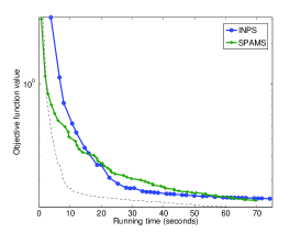
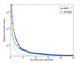
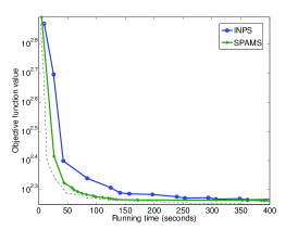
Figure 1: Running times of NIPS (Matlab) versus SPAMS (C++) for NMF on RAND, CBCL, and YALE datasets. Initial objective values and tiny runtimes have been suppressed for clarity of presentation.

On the NMF baseline (Fig. 1), we compare NIPS against the well optimized state-of-the-art C++ toolbox SPAMS (version 2.3) [Mairal et al. 2010]. We compare against SPAMS only on dense matrices, as its NMF code seems to be optimized for this case. Obviously, the comparison is not fair: unlike SPAMS, NIPS and its subroutines are all implemented in Matlab, and they run equally easily on large sparse matrices. Nevertheless, NIPS proves to be quite competitive: Fig. 1 shows that our Matlab implementation runs only slightly slower than SPAMS. We expect a well-tuned C++ implementation of NIPS to run at least 4–10 times faster than the Matlab version—the dashed line in the plots visualizes what such a mere 3X-speedup to NIPS might mean.

Figure 2 shows numerical results comparing the stochastic generalized gradient (SGGD) algorithm of [Ermoliev and Norkin 1998] against NIPS, when started at the same point. As in well-known, SGGD requires careful stepsize tuning; so we searched over a range of stepsizes, and have reported the best results. NIPS too requires some stepsize tuning, but substantially lesser than SGGD. As predicted, the solutions returned by NIPS have objective function values lower than SGGD, and have greater sparsity.

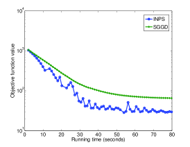
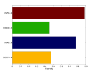
Figure 2: Sparse NMF: NIPS versus SGGD. The bar plots show the sparsity (higher is better) of the factors $X$ and $A$. Left plots for RAND dataset; right plots for WEB. As expected, SGGD yields slightly worse objective function values and less sparse solutions than NIPS.

5 Discussion

We presented a new framework called NIPS, which solves a broad class of nonconvex composite objective problems. NIPS permits nonvanishing computational errors, which can be practically useful. We specialized NIPS to also obtain a scalable incremental version. Our numerical experiments on large scale matrix factorization indicate that NIPS is competitive with state-of-the-art methods.

We conclude by mentioning that NIPS includes numerous other algorithms as special cases. For example, batch and incremental convex FBS, convex and nonconvex gradient projection, the proximal-point algorithm, among others. Theoretically, however, the most exciting open problem resulting from this paper is: extend NIPS in a scalable way when even the nonsmooth part is nonconvex. This case will require very different convergence analysis, and is left to the future.

Appendix A Implementation notes

If $\mathcal{X}$ is the nonnegative orthant $\mathbb{R}_{+}^{n}$, then the proximity operator $\operatorname{prox}_{\eta}^{g}$ often simplifies as

$$\operatorname{prox}_{\eta}^{g}(y)=\operatorname{prox}_{\eta}^{\psi}(\Pi_{\mathcal{X}}y).$$ (43)

Additionally, if $\psi$ is an elementwise separable function, then one can easily admit a box-plus-hyperplane constraint set $\mathcal{X}$ of the form

$$\mathcal{X}=\left\{{x\in\mathbb{R}^{n}\ |\ l_{i}\leq x_{i}\leq u_{i},\text{for }1\leq i\leq n,\ \text{and }a^{T}x=b}\right\}.$$ (44)

For more general constraint sets, we can invoke Dykstra splitting [Combettes and Pesquet, 2010], which solves the problem

$$\min\quad\tfrac{1}{2}\|{x-y}\|^{2}+\psi(x)+\delta(x|\mathcal{X}),$$ (45)

by using the following algorithm

Dykstra splitting for (45)
 Initialize $x\leftarrow y$, $p\leftarrow 0$, $q\leftarrow 0$
While $\neg$ converged, iterate:
$$\hskip-113.81102pt\left\lfloor\begin{array}[]{l@{\hspace{2pt}}l}e\hfil\hskip 2.0&\leftarrow\operatorname{prox}_{1}^{\psi}(x+p)\\ p\hfil\hskip 2.0&\leftarrow x+p-e\\ x\hfil\hskip 2.0&\leftarrow\Pi_{\mathcal{X}}(e+q)\\ q\hfil\hskip 2.0&\leftarrow e+q-x.\end{array}\right.$$ (46)

It can be shown that iterating (46) converges to the solution of (45). In practice, it usually suffices to run Dykstra splitting for a few iterations (2–10) only.

References

- Attouch et al. [2011] H. Attouch, J. Bolte, and B. F. Svaiter. Convergence of descent methods for semi-algebraic and tame problems: proximal algorithms, forward-backward splitting, and regularized Gauss-Seidel methods. Math. Programming Series A, Aug. 2011. Online First.
- Bach et al. [2011] F. Bach, R. Jenatton, J. Mairal, and G. Obozinski. Convex optimization with sparsity-inducing norms. In S. Sra, S. Nowozin, and S. J. Wright, editors, Optimization for Machine Learning. MIT Press, 2011.
- Beck and Teboulle [2009] A. Beck and M. Teboulle. A Fast Iterative Shrinkage-Thresholding Algorithm for Linear Inverse Problems. SIAM J. Imgaging Sciences, 2(1):183–202, 2009.
- Bertsekas [1999] D. P. Bertsekas. Nonlinear Programming. Athena Scientific, second edition, 1999.
- Bertsekas [2010] D. P. Bertsekas. Incremental Gradient, Subgradient, and Proximal Methods for Convex Optimization: A Survey. Technical Report LIDS-P-2848, MIT, August 2010.
- Boyd and Vandenberghe [2004] S. Boyd and L. Vandenberghe. Convex Optimization. Cambridge University Press, March 2004.
- Clarke [1983] F. H. Clarke. Optimization and nonsmooth analysis. John Wiley & Sons, Inc., 1983.
- Combettes and Pesquet [2010] P. L. Combettes and J. Pesquet. Proximal Splitting Methods in Signal Processing. arXiv:0912.3522v4, May 2010.
- Combettes and Wajs [2005] P. L. Combettes and V. R. Wajs. Signal recovery by proximal forward-backward splitting. Multiscale Modeling and Simulation, 4(4):1168–1200, 2005.
- Davis and Hu [2011] T. A. Davis and Y. Hu. The University of Florida Sparse Matrix Collection. ACM Transactions on Mathematical Software, 2011. To appear.
- Duchi and Singer [2009] J. Duchi and Y. Singer. Online and Batch Learning using Forward-Backward Splitting. J. Mach. Learning Res. (JMLR), Sep. 2009.
- Ermoliev and Norkin [1998] Y. M. Ermoliev and V. I. Norkin. Stochastic generalized gradient method for nonconvex nonsmooth stochastic optimization. Cybernetics and Systems Analysis, 34:196–215, 1998.
- Fukushima and Mine [1981] M. Fukushima and H. Mine. A generalized proximal point algorithm for certain non-convex minimization problems. Int. J. Systems Science, 12(8):989–1000, 1981.
- Gafni and Bertsekas [1984] E. M. Gafni and D. P. Bertsekas. Two-metric projection methods for constrained optimization. SIAM Journal on Control and Optimization, 22(6):936–964, 1984.
- Gaivoronski [1994] A. A. Gaivoronski. Convergence properties of backpropagation for neural nets via theory of stochastic gradient methods. Part 1. Optimization methods and Software, 4(2):117–134, 1994.
- Haykin [1994] S. Haykin. Neural Networks: A Comprehensive Foundation. Prentice Hall PTR, 1st edition, 1994.
- Kreutz-Delgado et al. [2003] K. Kreutz-Delgado, J. F. Murray, B. D. Rao, K. Engan, T.-W. Lee, and T. J. Sejnowski. Dictionary learning algorithms for sparse representation. Neural Computation, 15:349–396, 2003.
- Kundur and Hatzinakos [1996] D. Kundur and D. Hatzinakos. Blind image deconvolution. IEEE Signal Processing Magazine, 13(3), May 1996.
- Lee and Seung [2000] D. D. Lee and H. S. Seung. Algorithms for Nonnegative Matrix Factorization. In NIPS, 2000.
- Lee et al. [2005] K. Lee, J. Ho, and D. Kriegman. Acquiring linear subspaces for face recognition under variable lighting. IEEE Trans. Pattern Anal. Mach. Intelligence, 27(5):684–698, 2005.
- Liu and Ye [2009] J. Liu and J. Ye. Efficient Euclidean projections in linear time. In ICML, Jun. 2009.
- Mairal et al. [2010] J. Mairal, F. Bach, J. Ponce, and G. Sapiro. Online Learning for Matrix Factorization and Sparse Coding. JMLR, 11:10–60, 2010.
- Moreau [1962] J. J. Moreau. Fonctions convexes duales et points proximaux dans un espace hilbertien. C. R. Acad. Sci. Paris Sér. A Math., 255:2897–2899, 1962.
- Nesterov [2004] Y. Nesterov. Introductory Lectures on Convex Optimization: A Basic Course. Springer, 2004.
- Nesterov [2007] Y. Nesterov. Gradient methods for minimizing composite objective function. Technical Report 2007/76, Université catholique de Louvain, Sept. 2007.
- Rockafellar [1976] R. T. Rockafellar. Monotone operators and the proximal point algorithm. SIAM J. Control and Optimization, 14, 1976.
- Rockafellar and Wets [1998] R. T. Rockafellar and R. J.-B. Wets. Variational analysis. Springer, 1998.
- Solodov [1997] M. V. Solodov. Convergence analysis of perturbed feasible descent methods. J. Optimization Theory and Applications, 93(2):337–353, 1997.
- Solodov [1998] M. V. Solodov. Incremental gradient algorithms with stepsizes bounded away from zero. Computational Optimization and Applications, 11:23–35, 1998.
- Solodov and Zavriev [1998] M. V. Solodov and S. K. Zavriev. Error stability properties of generalized gradient-type algorithms. J. Optimization Theory and Applications, 98(3):663–680, 1998.
- Sra [2012] S. Sra. Nonconvex proximal-splitting: Batch and incremental algorithms. arXiv:1109.0258, Sep. 2012.
- Sung [1996] K.-K. Sung. Learning and Example Selection for Object and Pattern Recognition. PhD thesis, MIT, 1996.
- Xiao [2009] L. Xiao. Dual averaging method for regularized stochastic learning and online optimization. In NIPS, 2009.