Quantifying non-Markovianity of continuous variable Gaussian dynamical maps

Abstract

We introduce a non-Markovianity measure for continuous variable open quantum systems based on the idea put forward in H.-P. Breuer et al. Phys. Rev. Lett.103, 210401 (2009), i.e., by quantifying the flow of information from the environment back to the open system. Instead of the trace distance we use here the fidelity to assess distinguishability of quantum states. We employ our measure to evaluate non-Markovianity of two paradigmatic Gaussian channels: the purely damping channel and the quantum Brownian motion channel with Ohmic environment. We consider different classes of Gaussian states and look for pairs of states maximizing the backflow of information. For coherent states we find simple analytical solutions, whereas for squeezed states we provide both exact numerical and approximate analytical solutions in the weak coupling limit.

I Introduction

Physical systems are never perfectly isolated from their environment. Especially in quantum mechanics, when they are exploited to perform quantum computation or communication protocols, the interaction of the systems of interest with the environment should be considered in the derivation of the dynamical equations. Effects of this interaction, e.g. decoherence and disentanglement, can indeed endanger the accomplishment of any task based on quantum features like coherence or entanglement.

In order to take into account the presence of the environment and its influence on the dynamics of the system, within the theory of open quantum systems BrePet ; Weiss a variety of techniques have been developed to describe the evolution of the system of interest, e.g. by quantum master equations. The functional form of any master equation depends both on the system and environment, and on the specific features and strength of the interaction. In the literature the dynamics of open quantum systems are often described using master equations in the so-called Lindblad form LiGoKoSu . Profitable applications of this class of dynamical equations are present in many fields of physics, and systems whose dynamics is described by equations in the Lindblad form are generally called Markovian. As it will be explained in more detail in Sec. II, the dynamical maps associated with Lindblad master equations are divisible, implying that during the evolution any pair of initially different states becomes less and less distinguishable. This phenomenon is interpreted as an irreversible loss of information which flows from the system to the environment, and it is considered to be the key feature of Markovianity Bre09 .

In practice, however, Lindblad master equations are derived under a series of approximations. The exact dynamics of any physical system is generally described by other classes of master equations. Recently, a lot of effort has been devoted to provide a formal definition of non-Markovianity in open quantum systems, e.g. to capture physical features such as the re-coherence due to reservoir memory effects NMQJ ; pseudo . These efforts Wolf08 ; Bre09 ; Rivas10 also lead to computable measures for the degree of non-Markovianity. In this paper, we focus on the definition given in Ref. Bre09 where non-Markovianity is defined in terms of the information flow between the open system and its environment.

Besides its own importance from a purely theoretical point of view, the concept of non-Markovianity and its quantification may also find practical applications. One may ask indeed, whether non-Markovianity can be considered as a resource to improve quantum technologies. More specifically, assuming that the density of modes of the reservoir may be engineered in a controlled way to induce non-Markovian behavior, can this be used to improve existing quantum protocols? The first affirmative answers come from quantum metrology and quantum key distributon. In Ref. Chin11 the authors investigate the problem of parameter estimation when the quantum channel is non-Markovian according to the definition given in Ref. Rivas10 . They find that, for some non-Markovian reservoirs, the estimation can be improved compared to the Markovian case. The other example is reported in Ref. Vas11 where it has been proven that quantum key distribution protocols in non-Markovian channels provide alternative ways of protecting the communication which cannot be implemented in usual Markovian channels.

Even if the definition introduced in Ref. Bre09 is independent of the nature of the physical system, it has been applied so far to the discrete variable case only. In this paper we extend the analysis to continuous variable (CV) systems BraunRev which, in quantum information and communication, represent a valid, and sometimes better, alternative to discrete variable systems. Our aim is to introduce and study a computable measure for the degree of non-Markovianity in continuous variable systems focussing on some relevant examples of Gaussian preserving maps. Moreover we also consider the possibility of evaluating the map only for subsets of Gaussian states (e.g. coherent states and squeezed states) with the main intent to provide a characterization of the map for protocols relying only on those specific classes of states. This approach paves the way to a definition of non-Markovianity as a resource in quantum information theory.

The paper is organized as follows: in Sec. II we review the non-Markovianity measure we use and extend the definition to the realm of continuous variable Gaussian states. In Sec. III we focus on a phenomenological master equation describing a damping channel and evaluate its non-Markovianity, whereas in Sec. IV we address the same issue for quantum Brownian motion in the weak coupling limit. Finally in Sec. V we discuss the results and close the paper with some concluding remarks.

II Quantifying non-Markovianity in continuous variable systems

The measure for the degree of non-Markovianity of a quantum process introduced in Bre09 is based on the distinguishability of two different initial quantum states $\rho_{1}$ and $\rho_{2}$ under the action of the open system dynamical map $\Phi_{t}$ associated to the process. The distinguishability is qualified and quantified in Bre09 through the introduction of a proper distance measure between quantum states, the trace distance defined as $\mathcal{D}(\rho_{1},\rho_{2})=\hbox{Tr}|\rho_{1}-\rho_{2}|/2$. The trace distance satisfies a contractivity property under the action of any completely positive (CPT) map $\Phi$

$$\mathcal{D}(\rho_{1},\rho_{2})\geq\mathcal{D}(\Phi\rho_{1},\Phi\rho_{2}).$$ (1)

Given a dynamical map $\Phi_{t,t_{0}}$, this is called divisible if the evolution up to a time $t$ can be written as a completely positive evolution from the initial time $t_{0}$ to an intermediate time $\tau$, and another completely positive evolution from the intermediate time to the final time $t$, i.e. $\Phi_{t,t_{0}}=\Phi_{t,\tau}\cdot\Phi_{\tau,t_{0}}$, for any $t_{0}<\tau<t$. Lindblad dynamical semigroups LiGoKoSu describe divisible processes. It follows that under such dynamics the trace distance is always monotonic, i.e. $\mathcal{D}\bigl{(}\rho_{1}(\tau),\rho_{2}(\tau)\bigl{)}\geq\mathcal{D}\bigl{(}\rho_{1}(t),\rho_{2}(t)\bigl{)}$ for any pair $\rho_{1}(0)$, $\rho_{2}(0)$ of initial states and for any $t_{0}\leq\tau\leq t$. The monotonic decrease however holds also for classes of divisible maps which are not of a Lindblad form (examples are given in Bre09 ). On the other hand, the most dynamical evolutions violate both the divisibility condition and the monotonicity property of the trace distance. When monotonicity is not satisfied it means that there are intervals of time for which the states become more distinguishable compared to previous instants. This feature is interpreted as a flow of information from the environment back to the system, a striking property which characterizes a non-Markovian evolution. The measure of the degree of non-Markovianity is then defined as

$$\mathcal{N}=\max_{\rho_{1},\rho_{2}}\int_{\dot{\mathcal{D}}>0}\frac{d}{dt}\mathcal{D}(\rho_{1}(t),\rho_{2}(t))dt,$$ (2)

where $\dot{\mathcal{D}}$ indicates the time derivative and the maximization is taken over all the possible pairs of initial states.

So far the quantity in (2) has been evaluated and analyzed in some details for discrete variables quantum maps, e.g. a one qubit channel Bre09 ; Bas11 ; Znidaric11 . In this paper we extend it to continuous variable systems, focusing to single-mode systems. The extension involves two main issues requiring specific attention. The first comes from the fact that the Hilbert space for continuous variable systems is infinite dimensional, and therefore it is not possible to characterize all the states with a finite number of parameters as in the qubit case (e.g. Bloch sphere representation). The second issue is related to the lack of an analytic expression for the trace distance or other, equivalent, distance measures for a generic CV state. On the other hand, these issues may be solved upon restricting the analysis to Gaussian states, and Gaussian preserving channels Gauss . In fact, Gaussian states can be uniquely characterized by a finite number of parameters. Moreover, since analytic expressions for the trace distance are lacking, alternative distinguishability signatures may be employed within the same spirit. One possible choice is to use the fidelity

$$\mathcal{F}(\rho_{1},\rho_{2})=\hbox{Tr}\sqrt{\sqrt{\rho_{1}}\rho_{2}\sqrt{\rho_{1}}},$$ (3)

which is related to a proper distance measure, the Bures distance $\mathcal{D}_{\mathcal{F}}(\rho_{1},\rho_{2})=\sqrt{2-2\sqrt{\mathcal{F}(\rho_{1},\rho_{2})}}$. Remarkably, the fidelity, and, thus, also the Bures distance, are monotonic under the action of any CPT map, making it a good candidate for taking the role of the trace distance in the definition of the non-Markovian measure.

An alternative choice we could consider is the relative entropy $\mathcal{S}(\rho_{1}||\rho_{2})=\hbox{Tr}\bigl{[}\rho_{1}\log\rho_{1}-\rho_{1}\log\rho_{2}\bigl{]}$ whose expression for Gaussian states is known Mar04 . Despite the fact that also the relative entropy possesses a contractivity property under CPT maps, it is not a proper distance measure (e.g. it lacks symmetry property), and also it is not bounded. For these reasons we base our study on the fidelity.

The most general single-mode Gaussian state can be written as Gauss

$$\rho^{G}=D(\beta)S(\xi)\nu_{\rm th}(N)S^{{\dagger}}(\xi)D^{{\dagger}}(\beta)\,,$$

where $S(\xi)=\exp[\frac{1}{2}(\xi{a^{{\dagger}2}}-\xi^{*}a^{2})]$ and $D(\beta)=\exp[\beta a^{{\dagger}}-\beta^{*}a)]$ are the squeezing operator and the displacement operator, respectively, and $\nu_{\rm th}(N)=(N)^{a^{\dagger}a}/(1+N)^{a^{\dagger}a+1}$ is a thermal equilibrium state with $N$ average number of quanta, $a$ being the annihilation operator. Upon introducing the vector operator $\boldsymbol{R}^{T}=(R_{1},R_{2})\equiv(q,p)$, where $q=(a+a^{\dagger})/{\sqrt{2}}$ and $p=(a^{\dagger}-a)/(i\sqrt{2})$ are the so-called quadrature operators, we can fully characterize $\rho^{G}$ by means of the first moment vector

$$\overline{\boldsymbol{X}}^{T}=\langle\boldsymbol{R}^{T}\rangle=\sqrt{2}(\Re{\rm e}[\beta],\Im{\rm m}[\beta])\,,$$

where $\langle A\rangle=\hbox{Tr}[A\,\rho]$, and of the $2\times 2$ covariance matrix (CM) $\boldsymbol{\sigma}$, with elements

$$[\boldsymbol{\sigma}]_{hk}=\frac{1}{2}\langle R_{h}R_{k}+R_{k}R_{h}\rangle-\langle R_{h}\rangle\langle R_{k}\rangle\quad k=1,2\,.$$

The expression of the fidelity for a generic pair of Gaussian states $\rho_{1}^{G}$, $\rho_{2}^{G}$ can be given in a closed analytical form Scu98 and, as expected, depends only on the values of the vectors $\overline{\boldsymbol{X}}_{i}$, and covariance matrices $\boldsymbol{\sigma}_{i}$ of the states involved

$$\mathcal{F}(\rho^{G}_{1},\rho^{G}_{2})=\frac{2}{\sqrt{\Delta+\delta}-\sqrt{\delta}}\,e^{-\frac{1}{2}\overline{\boldsymbol{X}}^{T}(\boldsymbol{\sigma}_{1}+\boldsymbol{\sigma}_{2})^{-1}\overline{\boldsymbol{X}}},$$ (4)

where

$$\Delta =4\,\hbox{Det}(\boldsymbol{\sigma}_{1}+\boldsymbol{\sigma}_{2}),$$ (5)

$$\delta =16\left[\hbox{Det}(\boldsymbol{\sigma}_{1})-\frac{1}{4}\right]\left[\hbox{Det}(\boldsymbol{\sigma}_{2})-\frac{1}{4}\right].$$ (6)

The fidelity in Eq. (4) is a function of all the parameters that characterize the pair of Gaussian states: two complex displacement amplitudes $\beta_{i}=|\beta_{i}|e^{i\theta_{i}}$, two complex squeezing amplitudes $\xi_{i}=r_{i}e^{i\phi_{i}}$ and two real thermal parameters $N_{i}$. In order to simplify the notation used in the following we introduce here a set of collective arguments

$$\begin{split}&\mathbf{P_{N}}\equiv\{N_{1},N_{2}\}\,,\\ &\mathbf{P_{S}}\equiv\{r_{1},r_{2},\phi_{1},\phi_{2}\}\,,\\ &\mathbf{P_{C}}\equiv\{|\beta_{1}|,|\beta_{2}|,\theta_{1},\theta_{2}\}\,,\end{split}$$ (7)

and denote, e.g. by $\mathcal{F}(\{\mathbf{P_{C}},\mathbf{P_{N}}\},t)$ the fidelity between two mixed coherent states at time $t$ of the evolution. The full set of parameters is denoted by the symbol $\mathbf{P}$.

A non-Markovianity measure may be obtained by integrating the time derivative of the fidelity $\mathcal{F}(\mathbf{P},t)$ over the intervals in which it decreases. If the class of initial states is characterized by the set of parameters $\mathbf{P}$ the measure may be written as

$$\mathcal{N}_{\mathbf{P}}=\max_{\mathbf{P}}\,\biggl{[}-\int_{\dot{\mathcal{F}}<0}\frac{d}{dt}\mathbf{\mathcal{F}}(\mathbf{P},t)\,dt\biggl{]},$$ (8)

where $\dot{\mathcal{F}}$ indicates the time derivative and the maximization is taken over the set of parameters $\mathbf{P}$.

The measure $\mathcal{N}_{\mathbf{P}}$ in (8) is obtained by maximization over the class of Gaussian states, a procedure which makes it particularly suitable to asses Gaussian preserving channels. On the other hand, when applied to a generic channel, it cannot be considered as a global property. This is not a crucial issue for practical applications for at least two reasons. On the one hand, this choice allows to actually calculate and compare the degree of non-Markovianity for continuous variable channels, a task that would not be feasible for non-Gaussian states. On the other hand, it should be noticed that while in principle there are techniques to prepare any kind of single qubit states, the same does not apply to continuous variable systems. As a matter of fact the class of Gaussian states plays a crucial role in quantum information processing, since they can be characterized theoretically in a convenient way, and they can also be generated and manipulated experimentally in a variety of physical systems, ranging from light fields to atomic ensembles. Therefore, our aim in the rest of the paper will be that of characterizing the Gaussian degree of non-Markovianity for some relevant Gaussian preserving channels.

Once we restrict the investigation to Gaussian states we still have to face the problem of the maximization procedure, which may be challenging from the numerical point of view, since the domains of some of the involved parameters are unbounded. One way to deal with this issue is to focus on subclasses of Gaussian states, e.g. pure coherent states or squeezed states, and therefore reduce the number of parameters involved. On the other hand, it is also possible to bound the domain of definition of the parameters, invoking the same line of reasoning used previously: experimental accessibility. For example, in practice it is not possible to obtain an arbitrary amount of squeezing Ebe10 . The consequence is then a limitation of the domain of definition and therefore a faster convergence of numerical maximization algorithms. In the cases we examine in the next sections however we will see that it is not always needed to bound the domain of definition of the parameters. This is because the maximizing pair of states depends on the strength of the interaction, i.e., the coupling constant, and for weakly coupled systems, experimentally accessible values for the squeezing and displacement may characterize the maximizing pair.

In the following Sections we will assume that the maximum is achieved for pure states, i.e., we assume $N_{1}=N_{2}=0$ and perform the maximization over the other parameters. This assumption may be proved for the case of coherent thermal states in the weak coupling regime, whereas we conjecture its validity for the other classes of states.

In the next two sections we introduce two different examples of master equations used to describe the dynamics of continuous variable systems and we study their non-Markovian Gaussian properties.

III Damping master equation

We start by considering the dynamics described by the following phenomenological Lindblad type equation with a single decay channel and a time dependent damping rate $\gamma(t)$,

$$\frac{d\rho}{dt}=\alpha\frac{\gamma(t)}{2}(2a\rho a^{{\dagger}}-a^{{\dagger}}a\rho-\rho a^{{\dagger}}a)\,.$$ (9)

Any Gaussian state evolving according Eq. (9) remains Gaussian, with the displacement and the covariance matrix evolving as follows Gauss

$$\beta(t) =e^{-\frac{x(t)}{2}}\beta(0),$$ (10)

$$\sigma(t) =e^{-x(t)}\sigma(0)+\left[1-e^{-x(t)}\right]\frac{\mathbb{I}}{2},$$

where

$$x(t)=\alpha\int_{0}^{t}2\gamma(s)ds,$$ (11)

and $\alpha$ being a coupling constant. If $x(t)\ll 1$ then we can approximate $e^{-x(t)}\simeq 1-x(t)$. Under this weak coupling condition we can also approximate the solution of (9) as follows

$$\begin{split}&\beta(t)=\biggl{[}1-\frac{x(t)}{2}\biggl{]}\beta(0),\\ &\sigma(t)=\bigl{[}1-x(t)\bigl{]}\sigma(0)+x(t)\,\frac{\mathbb{I}}{2}\,.\end{split}$$ (12)

Upon inserting Eq. (LABEL:EvoDamMEWC) into Eq. (4) we obtain the expression for the fidelity in the weak coupling limit. The divisibility property of (9) here is equivalent to the condition $\gamma(t)\geq 0$ for any $t\geq 0$, as it can be easily verified from the solution (10). On the other hand, the condition for non-Markovianity can be studied by inspecting the derivative of the fidelity with respect to time. Because the evolution of any Gaussian state depends on time through the function $x(t)$ only, we have

$$\frac{d\mathcal{F}}{dt}=\frac{d\mathcal{F}}{dx}\frac{dx}{dt}=2\alpha\gamma(t)\frac{d\mathcal{F}}{dx}.$$ (13)

If $\gamma(t)=\gamma_{0}>0$ and therefore $x_{M}(t)=2\alpha\gamma_{0}t$, then expression (13) must always be positive, because the dynamics is described by a divisible map. Therefore for any $t>0$ and any initial pair of states we must have $\frac{d\mathcal{F}}{dx}>0$. Because the image sets of $x(t)$ and $x_{M}(t)$ are the same, the condition $\frac{d\mathcal{F}}{dx}>0$ must hold also in the case of a time dependent decay rate. Stated in another way, Eq. (9) describes a non-Markovian channel if and only if the corresponding dynamical map is non-divisible. This condition is valid for any pair of initial states. The amount of non-Markovianity of the channel, as defined by Eq. (8), can be written as

$$\mathcal{N}_{\mathbf{P}}=\max_{\mathbf{P}}\sum_{I}\bigl{[}\mathcal{F}(\mathbf{P},t^{+}_{I})-\mathcal{F}(\mathbf{P},t^{-}_{I})\bigl{]},$$ (14)

where $[t^{+}_{I},t^{-}_{I}]$ is the $I$-th negativity interval of $\gamma(t)$.

For coherent states we may derive an exact expression for non-Markovianity valid for any form of the damping rate. Assuming a single interval of negativity, we have

$$\begin{split}&\mathcal{N}_{\mathbf{P_{C}}}=\exp\bigl{\{}-Ke^{-x(t^{+})}\bigl{\}}-\exp\bigl{\{}-Ke^{-x(t^{-})}\bigl{\}},\\ &K=\frac{|\beta_{1}e^{i\theta_{1}}-\beta_{2}|^{2}}{2}=\frac{x(t^{-})-x(t^{+})}{e^{-x(t^{+})}-e^{-x(t^{-})}}\,,\end{split}$$ (15)

where only one angle appears in the parameter $K$ because the master equation is invariant under a rotation in phase space. Other analytic results can be also obtained if we consider small values of the coupling constant. For example in the case of coherent states and for any number of negativity periods of the damping rate, we have

$$\begin{split}\mathcal{N}_{\mathbf{P_{C}}}&\simeq\max_{\mathbf{P}_{C}}\sum_{I}\bigl{[}e^{-[1-x(t^{+}_{I})]K}-e^{-[1-x(t^{-}_{I})]K}\bigl{]}\\ &=\max_{\mathbf{P}_{C}}e^{-K}\sum_{I}\bigl{[}e^{x(t^{+}_{I})K}-e^{x(t^{-}_{I})K}\bigl{]}\\ &=\alpha\,\biggl{\{}\max_{\mathbf{P_{C}}}f_{1}(\mathbf{P_{C}})\biggl{\}}\,\int_{\gamma<0}\!\!2\gamma(t)\,dt+o(\alpha^{2}),\end{split}$$ (16)

where we define the state dependent function $f_{1}(\mathbf{P_{C}})=e^{-K}K$. From Eq. (16) we can conclude that to first order in the coupling $\alpha$, the quantity $\mathcal{N}_{\mathbf{P}_{C}}$ is proportional to the integral of the negativity region of the damping rate, and the next contribution appears only to third order. The measure is then maximized for $K=1$, a condition which defines a whole set of pairs of states, all of them leading to the same value of $\mathcal{N}_{\mathbf{P}_{C}}$ to first order in $\alpha$. We then conclude that the degree of non-Markovianity for the set of coherent states can be written as

$$\begin{split}\mathcal{N}_{\mathbf{P_{C}}}=\frac{2}{e}\alpha\int_{\gamma<0}\!\!\gamma(t)\,dt+o(\alpha^{2})\,.\end{split}$$ (17)

This result has actually been derived under the hypothesis that also $e^{x(t^{\pm}_{I})K}\simeq 1+x(t^{\pm}_{I})K$ for any interval $I$, therefore limiting the parameter domain depending on the value of $\gamma(t)$ and $\alpha$. However, in the weak coupling limit the domain is large enough to contain the points for which $K=1$.

We now turn to the class of pure squeezed vacuum states (from now on referred to as squeezed states), characterized by the set of parameters $\mathbf{P_{S}}\equiv\{r_{1},r_{2},\phi_{1},\phi_{2}\}$, which, in the absence of displacement, can be reduced to $\mathbf{P_{S}}\equiv\{r_{1},r_{2},\phi,0\}$, with $\phi$ the angle between the squeezing directions. We can follow the same line of reasoning used previously for coherent states and, e.g. for a single period of negativity of the damping coefficient $[t^{+},t^{-}]$, define the quantity

$$\begin{split}\mathcal{N}_{\mathbf{P_{S}}}&=\max_{\mathbf{P_{S}}}\bigl{[}\mathcal{F}(\mathbf{P_{S}},t^{+})-\mathcal{F}(\mathbf{P_{S}},t^{-})\bigl{]}\\ &=\alpha\,\biggl{\{}\max_{\mathbf{P_{S}}}g_{1}(\mathbf{P_{S}})\biggl{\}}\int_{\gamma<0}\!\!2\gamma(t)\,dt+o(\alpha)\,,\end{split}$$ (18)

where function $g_{1}(\mathbf{P_{S}})$ depends on the parameters $r_{1},r_{2}$ and $\phi$ in a rather complicated way. Its expression can be simplified if we set $r=r_{1}=r_{2}$

$$g_{1}(\mathbf{P_{S}})=8\cosh(2r)\frac{k(r,\phi)-\sqrt{k(r,\phi)}}{k^{2}(r,\phi)},$$ (19)

where $k(r,\phi)=3+\cos\phi+\cosh 4r(1-\cos\phi)$. We will discuss later on in this Section about the maximization of the function $g_{1}(\mathbf{P_{S}})$.

From Eq. (18) we notice that the second order term is not zero for squeezed states, suggesting that the first order approximation has a more limited validity than in the case of coherent states. It is also nontrivial to determine the domain of parameters which allows the expansion to be truncated at first order. This is due to the more complicated functional form of the fidelity when squeezing, instead of displacement is implemented. The first order result is then of a similar form to the coherent state case, with a different state dependent coefficient $g_{1}(\mathbf{P_{S}})$. It is straightforward to show that this result is independent of the number of negativity periods of $\gamma(t)$.

Interesting results can be also derived if we consider now the most general pure Gaussian state (both displacement and squeezing). From (4) we can separate the fidelity as a product of two parts $\mathcal{F}(\{\mathbf{P_{C}},\mathbf{P_{S}}\},t)=C(\{\mathbf{P_{C}},\mathbf{P_{S}}\},t)S(\mathbf{P_{S}},t)$, where $C(\{\mathbf{P_{C}},\mathbf{P_{S}}\},t)$ is the exponential part, containing the coherent state amplitudes, and $S(\mathbf{P_{S}},t)$ is the fidelity for zero displacement. A first order expansion in $\alpha$ shows that

$$\begin{split}&\mathcal{N}_{\{\mathbf{P_{C}},\mathbf{P_{S}}\}}=\alpha\int_{\gamma<0}\!\!2\gamma(t)\,dt\\ &\times\max_{\{\mathbf{P_{C}},\mathbf{P_{S}}\}}\bigl{\{}S(\mathbf{P_{S}},0)f_{1}(\mathbf{P_{C}})+C(\{\mathbf{P_{C}},\mathbf{P_{S}}\},0)g_{1}(\mathbf{P_{S}})\bigl{\}}\\ &+o(\alpha).\end{split}$$ (20)

This result gives the non-Markovianity measure at first order in $\alpha$ with a pair dependent coefficient given by a linear combination of the displacement contributions $f_{1}(\mathbf{P_{C}})$ and the squeezing one $g_{1}(\mathbf{P_{S}})$. However, we cannot conclude that even at this order the two contribution are completely independent, because the weights appearing in the combination depend on the fact that we applied squeezing and displacement. For example it is easy to show that $S(\mathbf{P_{S}},0)=\mathcal{F}(\mathbf{P_{S}},0)$ is the initial fidelity of the same pair of states with zero displacement, and $C(\{\mathbf{P_{C}},\mathbf{P_{S}}\},t)=\mathcal{F}(\{\mathbf{P_{C}},\mathbf{P_{S}}\},0)/\mathcal{F}(\mathbf{P_{S}},0)$, is the ratio between the initial fidelity and the initial fidelity without displacement.

It is worth noticing that for coherent-thermal states with equal thermal parameters, i.e. $N_{1}=N_{2}=N$, at first order in the coupling we obtain

$$\begin{split}\mathcal{N}_{\{\mathbf{P_{N}},\mathbf{P_{C}}\}}&=\max_{N\geq 0}\frac{\mathcal{N}_{\mathbf{P_{C}}}}{2N+1}+o(\alpha^{2}),\end{split}$$ (21)

which is maximized by pure states ($N=0$), thus supporting our choice to restrict the analysis to pure states only.

As we mentioned before many features of non-Markovianity for the damping channels do not depend on the specific form of the damping rate. However, for the sake of concreteness let us now consider an example of the damping rate

$$\begin{split}&\gamma(t)=\frac{1}{2}\biggl{\{}\begin{array}[]{c}e^{-t/10}\sin t,\\ e^{-\pi/4},\\ \end{array}\qquad\begin{array}[]{c}{\rm if}\\ {\rm if}\end{array}\qquad\begin{array}[]{c}t<5\pi/2,\\ t\geq 5\pi/2,\end{array}\end{split}$$ (22)

which is characterized by only one interval of negativity, $[\pi,2\pi]$, and where we are definitely in the weak coupling regime if $\alpha\lesssim 0.1$.

We start the analysis evaluating the non-Markovianity of the channel for coherent states and squeezed states. These results are shown in Fig.1, where we plot for both classes the non-Markovianity evaluated at first order, together with the exact numerical solution obtained by maximizing (14) using the full solution (10).

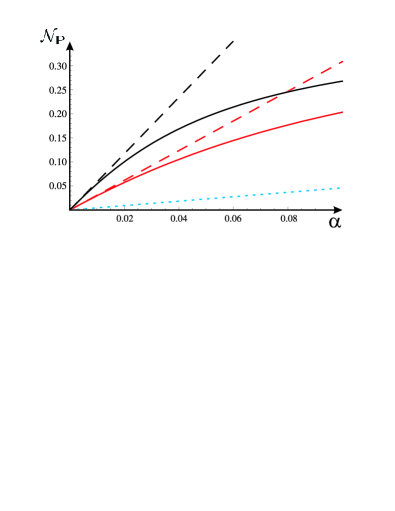
Figure 1: (Color online) Non-Markovianity of the purely damping channel as a function of the coupling $\alpha$. The dotted blue line is the result obtained by maximizing over coherent states (the exact solution and the first order approximation coincides). The solid lines are the exact non-Markovianities for squezeed states, whereas the dashed lines are the corresponding first order approximations. Black curves correspond to $\phi=0.2$,while red ones to $\phi=0.1$.

The coherent states maximization has been carried out over all the parameters involved and their domain, while for squeezed states we consider two fixed values of the angle $\phi$ between the squeezing directions and then maximize over the magnitudes $r_{1}$ and $r_{2}$, with the maximum value reached for $r_{1}=r_{2}$. Two main results are evident: the non-Markovianity of the damping channel is larger for squeezed states than for coherent states independently of the value of coupling and increases with decreasing $\phi$. Due to the nature of the master equation we can also state that this result is valid independently of the form of $\gamma(t)$. The second result is that the first order approximation is well sustained by coherent states while it is violated by squeezed states also for relatively small values of the coupling. This behavior for squeezed states becomes more and more evident if we reduce the value of the angle $\phi$, and it can be explained by inspecting Eq. (19) for fixed $\phi>0$. For small $\phi$, in fact, the function $g_{1}(\mathbf{P_{S}})$ decreases, thus determining a violation of the first order approximation. A further discussion of the results is postponed to the final Section, after we have provided a more complete picture by discussing the quantum Brownian motion model in the next Section.

IV Quantum Brownian motion

The master equation describing quantum Brownian motion (QBM) in the interaction picture, under the weak coupling and secular approximations (see, e.g. Ref. QBMEq and references therein), is given by

$$\begin{split}\frac{d\rho}{dt}&=\alpha\,\frac{\Delta(t)+\gamma(t)}{2}(2a\rho a^{{\dagger}}-a^{{\dagger}}a\rho-\rho a^{{\dagger}}a)\\ &+\alpha\,\frac{\Delta(t)-\gamma(t)}{2}(2a^{{\dagger}}\rho a-aa^{{\dagger}}\rho-\rho aa^{{\dagger}}).\end{split}$$ (23)

The diffusion and damping coefficients $\Delta(t)$ and $\gamma(t)$ can be derived once we provide the analytic form of the spectral density $J(\omega)$ and the temperature $T$ of the environment, assumed to be in a thermal state. Their expressions in the weak coupling limit are

$$\begin{split}&\Delta(t)=\int_{0}^{t}\!\!ds\int_{0}^{\infty}\!\!\!d\omega\,J(\omega)\biggl{(}N(\omega)+\frac{1}{2}\biggl{)}\cos(\omega_{0}s)\cos(\omega s),\\ &\gamma(t)=\int_{0}^{t}\!\!ds\int_{0}^{\infty}\!\!d\omega\,J(\omega)\sin(\omega_{0}s)\sin(\omega s),\end{split}$$ (24)

where $N(\omega)=(\exp\{\hbar\omega/k_{B}T\}-1)^{-1}$ is the mean number of thermal photons for a mode of frequency $\omega$, and $\omega_{0}$ is the bare frequency of the system. The spectral function we are going to consider is the following Ohmic spectral density

$$J(\omega)\propto\omega\,C(\omega,\omega_{c})\,,$$ (25)

where $C(\omega,\omega_{c})$ is a high frequency cutoff function with $\omega_{c}$ being the cutoff frequency. Usually the cutoff function is chosen to be of Lorentzian or exponential form. Here we use an exponential cutoff $C(\omega,\omega_{c})=\exp\{-\omega/\omega_{c}\}$, such that

$$J(\omega)=\omega e^{-\omega/\omega_{c}}\,.$$ (26)

The exact solution of Eq. (23) for the displacement and covariance matrix of any initial Gaussian state is

$$\begin{split}&\beta(t)=e^{-\frac{1}{2}x(t)}\beta(0),\\ &\sigma(t)=e^{-x(t)}\sigma(0)+\alpha\,\frac{\mathbb{I}}{2}e^{-x(t)}\int_{0}^{t}e^{x(s)}\Delta(s)ds\,,\end{split}$$ (27)

which, at first order in $\alpha$ can be written as

$$\begin{split}&\beta(t)=\biggl{[}1-\frac{x(t)}{2}\biggl{]}\beta(0)\\ &\sigma(t)=\bigl{[}1-x(t)\bigl{]}\sigma(0)+y(t)\frac{\mathbb{I}}{2},\end{split}$$ (28)

with

$$x(t)=2\alpha\int_{0}^{t}\!\!\gamma(s)\,ds,\quad y(t)=2\alpha\int_{0}^{t}\!\!\Delta(s)\,ds\,,$$

and where $\sigma(0)$ and $\beta(0)$ are the covariance matrix and displacement vector of the initial state, respectively.

The dynamics generated by Eq. (23) is more involved compared to that of Eq. (9), and this gives us the opportunity to study in more detail the non-Markovianity properties of continuous variable systems. What is here relevant, compared to the previous case, is the presence of two decay channels, one downward channel and one upward. This structure leads to the inequivalence of non-divisibility and non-Markovianity. For the master equation (23) the divisibility property is satisfied if $\Delta(t)\geq|\gamma(t)|$ Bre09 . On the other hand, we have a non-Markovian behavior if the following quantity attains negative values

$$\frac{d\mathcal{F}}{dt}=\frac{\partial\mathcal{F}}{\partial x}\frac{dx}{dt}+\frac{\partial\mathcal{F}}{\partial y}\frac{dy}{dt}=2\alpha\gamma(t)\frac{\partial\mathcal{F}}{\partial x}+2\alpha\Delta(t)\frac{\partial\mathcal{F}}{\partial y}.$$ (29)

The sign of (29) depends in a non trivial way on the values of the damping and diffusion coefficients, and of the derivatives of the fidelity with respect to $x(t)$, $y(t)$, which are in general functions of all the parameters and the time. Expression (29) indicates that both damping and diffusion phenomena contribute to the process. The dominance between the two contributions depends on the spectral function $J(\omega)$, the coupling constant, the temperature of the environment and on the initial pair of states through the derivatives $\partial\mathcal{F}/\partial x$ and $\partial\mathcal{F}/\partial y$. Each derivative is proportional to the difference between two fidelities, the one calculated for an increment in one variable and the initial one. We expect that, e.g. $\mathcal{F}(x+h,y)>\mathcal{F}(x,y)$ holds, because, according to Eq. (LABEL:EvoQbmME), the first term is the fidelity between two states which have lost information about their initial preparation [see Eq. (LABEL:EvoQbmME)]. In other words, we expect non-Markovianity to be dependent on the sign of the master equation coefficients and only on the magnitude of the partial derivatives.

Numerical evaluation of the region of negativity of $d\mathcal{F}/dt$ shows that the zeroes of the derivative are essentially the same as those of the diffusion coefficient $\Delta(t)$, thus suggesting that diffusion is the leading phenomenon for non-Markovianity of QBM. In order to prove this result we should inspect the form of the non-Markovianity at the first order in the coupling $\alpha$, in the same spirit as in Sec. III. For coherent states we have

$$\begin{split}\mathcal{N}_{\mathbf{P}_{\mathbf{C}}}=\frac{2}{e}\alpha\int_{\Delta<0}\!\!\Delta(t)\,dt+o(\alpha^{2}),\end{split}$$ (30)

and the contribution from the damping coefficient appears only in the third power of the coupling. For squeezed states we get

$$\begin{split}\frac{d\mathcal{F}}{dt}&=\alpha S_{\Delta}(r_{1},r_{2},\phi)\Delta(t)+\alpha S_{\gamma}(r_{1},r_{2},\phi)\gamma(t)+o(\alpha^{2}),\end{split}$$ (31)

where the coefficients $S_{\gamma}(r_{1},r_{2},\phi)$ and $S_{\Delta}(r_{1},r_{2},\phi)$ are the zeroth order expansions of the derivatives $d\mathcal{F}/dx$ and $d\mathcal{F}/dy$, respectively. An inspection on the magnitudes of the coefficients shows, however, that unless $\phi\simeq 1$ (the maximum of the measure is instead obtained in the region $\phi\ll 1$), we have $S_{\gamma}(r_{1},r_{2},\phi)\ll S_{\Delta}(r_{1},r_{2},\phi)$. Therefore, non-Markovianity can be approximated by

$$\begin{split}\mathcal{N}_{\mathbf{P}_{\mathbf{S}}}=\alpha\max_{r_{1},r_{2},\phi}S_{\Delta}(r_{1},r_{2},\phi)\int_{\Delta<0}\!\!2\Delta(t)\,dt+o(\alpha^{2}).\end{split}$$ (32)

Within the validity of the first order expansion this explains why the zeros of (29) essentially coincides with those of $\Delta(t)$.

As for the damping channel, it is possible to derive a closed formula for the non-Markovianity of QBM for coherent states. The only assumption is that the negativity of the derivative of the fidelity coincides with the negativity of the diffusion coefficient. For a single interval of negativity we have

$$\mathcal{N}_{\mathbf{P_{C}}}= \exp\left\{-\frac{Pe^{-x(t^{+})}}{e^{-x(t^{+})}+y(t^{+})}\right\}$$

$$- \exp\left\{-\frac{Pe^{-x(t^{-})}}{e^{-x(t^{-})}+y(t^{-})}\right\},$$ (33)

where

$$P =\frac{|\beta_{1}e^{i\theta_{1}}-\beta_{2}|^{2}}{2}=\ln\biggl{[}\frac{e^{-x(t^{+})}}{e^{-x(t^{-})}}\frac{e^{-x(t^{-})}+y(t^{-})}{e^{-x(t^{+})}+y(t^{+})}\biggl{]}$$ (34)

$$\times\biggl{(}\frac{e^{-x(t^{+})}}{e^{-x(t^{+})}+y(t^{+})}-\frac{e^{-x(t^{-})}}{e^{-x(t^{-})}+y(t^{-})}\biggl{)}^{-1}.$$

Because the non-Markovianity is here led by the diffusion phenomena, we expect a strong dependence also on the temperature of the environment. In the following, we will examine the non-Markovianity in different temperature regimes, comparing the first order approximation and the numerical one based on the exact solution (LABEL:EvoQbmEx).

The temperature dependence of the diffusion coefficients is apparent in its definition (LABEL:CoeffME). Essentially the coefficient is a sum of a zero temperature term and a contribution from the thermal photons in the bath. Respectively, their expressions are

$$\begin{split}&\Delta_{0}(t)=\frac{1}{2}\int_{0}^{t}ds\int_{0}^{\infty}d\omega J(\omega)\cos(\omega_{0}s)\cos(\omega s),\\ &\Delta_{T}(t)=\int_{0}^{t}ds\int_{0}^{\infty}d\omega J(\omega)N(\omega)\cos(\omega_{0}s)\cos(\omega s).\end{split}$$ (35)

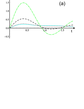
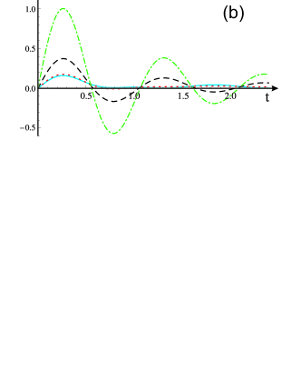
Figure 2: (Color online) Diffusion coefficients as a function of time for an Ohmic environment with $\omega_{c}=1$ and (a): $\omega_{0}=4$, (b): $\omega_{0}=6$. We plot the zero temperature diffusion coefficient (solid blue), low temperature ($k_{B}T/\hbar\omega_{c}=1/5$, red dotted), intermediate temperature ($k_{B}T/\hbar\omega_{c}=1$, black dashed) and high temperature ($k_{B}T/\hbar\omega_{c}=4$, green dotted-dashed line).

For low temperature, that is when the thermal energy $k_{B}T$ is much smaller than any excitation energy, $\hbar\omega_{0},\hbar\omega_{c}$, the total coefficient does not differ much from the zero temperature contribution. Therefore we expect non-Markovianity to be independent of $T$ in this regime. As $T$ is increased $\Delta_{T}(t)$ starts to become relevant and in the high temperature regime becomes dominant compared to $\Delta_{0}(t)$. In this regime the coefficient depends linearly on $T$ and therefore we can expect a strong dependence of non-Markovianity on temperature. Another feature is illustrated in Fig. 2, where we show the diffusion coefficients for different values of the bare frequency $\omega_{0}$. By comparing the two panels, we can see that if we approach the resonance condition $\omega_{c}\simeq\omega_{0}$, the diffusion coefficient at low temperature does not show negative regions and so the first order non-Markovianity is vanishing. As we increase the temperature, $\Delta(t)$ may become negative and therefore the system shows a non-Markovian behavior. This distinction between low and high temperature ceases to be valid when we are out of resonance $\omega_{c}/\omega_{0}\ll 1$, where also for low temperature we can have a non-Markovian behavior.

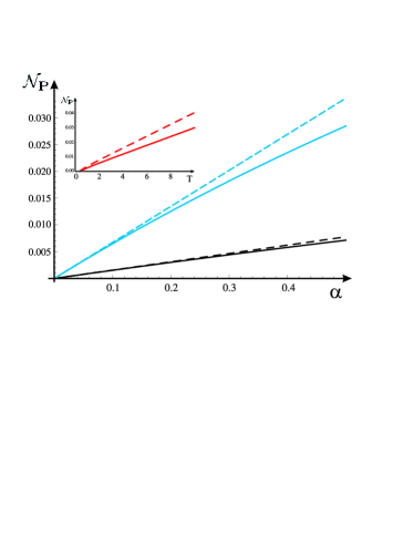
Figure 3: (Color online) Non Markovianity of QBM channel with Ohmic reservoir on coherent states as a function of the coupling $\alpha$ with $\omega_{c}=0.2$ and $\omega_{0}=1$, for different temperatures. Dashed (solid) lines represent the first order approximate (numerical) solutions. Black curves correspond to $k_{B}T/\hbar\omega_{0}=0.2$ and blue curves to $k_{B}T/\hbar\omega_{0}=0.5$. The inset shows the temperature dependence for fixed coupling $\alpha=0.1$, and $\omega_{0}=1$ (red solid), $\omega_{0}=1.1$ (red dashed).

After this discussion on the nature and behavior of the diffusion coefficient, we are ready to illustrate the results about non-Markovianity of the QBM channel. We start by considering the class of coherent states, for which the first order measure is defined in Eq.(30). In Fig. 3 we show the comparison between the analytic and numerical results for $\omega_{c}=0.1$ and $\omega_{0}=1$, and for two different values of temperature. When $\alpha<0.1$ the agreement is good in both cases, whereas the first order approximation fails for the higher temperature when we increase the coupling. In the inset of Fig. 3 we show the first order measure for fixed coupling ($\alpha=0.1$) as a function of the temperature when $\omega_{c}=0.3$ and different values of $\omega_{0}$. When $T<0.4$ the measure is zero indicating that the diffusion coefficient has no negativity regions.

For squeezed states, in Fig. 4 we show the comparison between the numerical and first order analytic results for the measure as a function of the coupling constant $\alpha$ for small values of the temperature. We can notice a behavior similar to that of the damping channel case (See Fig. 2a), the exact and approximated expressions indeed coincide only for very small value of the coupling.

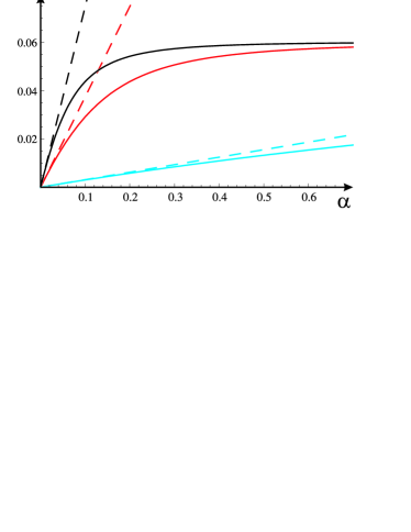
Figure 4: (Color online) Non-Markovianity of QBM channel with Ohmic reservoir as a function of $\alpha$. We have set $k_{B}T/\hbar\omega_{0}=0.2$, $\omega_{c}=0.2$, $\omega_{0}=1$. Red and black curves show the behavior of squeezed states, blue curves are for coherent states. Dashed (solid) curves represent the first order (numerical) solution to the maximization problem. For squeezed states the maximization has been performed with the constraint $r_{1}=r_{2}$ and for fixed phase $\phi=0.1$ (red curves), or $\phi=0.05$ (black curves). For coherent states the maximization has been performed over all their characterizing parameters.

For increasing $\alpha$ the non-Markovianity saturates to a constant value, which is achieved for smaller $\alpha$ when $\phi$ decreases. In Fig. 4 we compare the results for coherent and squeezed states, showing that also for the QBM channel squeezed states are more sensitive than coherent states to the non-Markovianity of the channel.

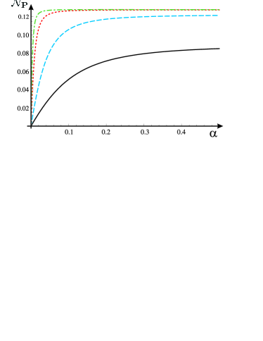
Figure 5: (Color online) Non Markovianity of QBM channel with Ohmic reservoir on coherent states. We have set $\omega_{c}=0.2$, $\omega_{0}=1$ and maximized at fixed angle $\phi=0.05$ over the squeezing parameters. Different lines correspond to different temperatures: $k_{B}T/\hbar\omega_{0}=0.3$ (black solid), $k_{B}T/\hbar\omega_{0}=0.9$ (blue dashed), $k_{B}T/\hbar\omega_{0}=4$ (red dotted) and $k_{B}T/\hbar\omega_{0}=8$ (green dotted dashed).

Finally in Fig. 5 we plot for fixed parameters $\omega_{c}=0.2$, $\omega_{0}=1$ and $\phi=0.05$ the numerical results for the measure for different temperatures. The behavior is qualitatively the same, i.e. we have saturation for increasing $\alpha$ and the saturation value increases with temperature, until it reaches a maximum saturation value for high temperatures.

V Discussion and conclusions

In the previous Sections we have analyzed in detail the non-Markovianity of two kinds of CV quantum channels, addressing separately the non-Markovian behavior for coherent and squeezed states. The dynamics of coherent states is governed by the evolution of only the displacement amplitude in the damping channels, and by both the displacement and the covariance matrix in the QBM channel case. On the the other hand, the dynamics of (zero amplitude) squeezed states depends on the covariance matrix only in both cases. This behavior allows us to address the effects of the two contributions on the amount of non-Markovianity of the channel.

Despite the difference in the form of the master equations, many common features are apparent. At first, we notice that squeezed states are in general more sensitive to the non-Markovian behavior, as witnessed by the larger non-Markovianity compared to coherent states, independently on the value of the coupling and temperature. Generally, for both classes of states, the non-Markovianity is mostly related to the sign of the master equation coefficients. For the case of QBM non-Markovianity is mostly due to diffusion described by the coefficient $\Delta(t)$. On the other hand, even if the dynamics of the displacement vector is not affected by it [see Eq. (LABEL:EvoQbmEx)], it is still fundamental for the class of coherent states. This behavior is even more evident as the temperature is increased, since the damping is independent of temperature.

Another interesting feature is the behavior of the non-Markovianity for squeezed states as a function of the coupling and the temperature, in particular for what concerns the quantum Brownian motion case. As it is apparent from Fig. 5, the value of non-Markovianity as a function of the coupling saturates, with a saturation value that increases with the temperature. This behavior, whose origin may be traced back to the time evolution of the covariance matrices, implies the existence of some bound on the flow of information from the environment back to the open system as a result of the Gaussian structure of the map.

In conclusion, we have introduced a measure to quantify the non-Markovianity of continuous variable quantum channels and have used it to analyze two paradigmatic Gaussian channels: the purely damping channel and the quantum Brownian motion channel with Ohmic environment. We have considered different classes of Gaussian states and found the pairs of states maximizing the backflow of information. For coherent states we have found analytical solutions, whereas for squeezed states we have resorted to numerical maximization, and also obtained some approximate analytical solutions in the weak coupling limit.

Our results are encouraging enough to suggest the use of our measure of non-Markovianity to analyze more general Gaussian channels, and to assess non-Markovianity as a resource for quantum technologies.

References

- (1) H. P. Breuer and F. Petruccione, The Theory of Open Quantum Systems (Oxford University Press, Oxford, 2002).
- (2) U. Weiss, Quantum Dissipative Systems (3rd Edition), (World Scientific, Singapore, 2008).
- (3) G. Lindblad, Commn. Math. Phys., 48, 119-130 (1976); V. Gorini, A. Kossakowski, and E.C.G. Sudarshan, J. Math. Phys. 17, 821-825 (1976).
- (4) H.-P. Breuer, E.-M. Laine, and J. Piilo, Phys. Rev. Lett. 103, 210401 (2009); E.-M. Laine, J. Piilo, and H.-P. Breuer, Phys. Rev. A 81, 062115 (2010).
- (5) J. Piilo, S. Maniscalco, K. Härkönen, and K.-A. Suominen Phys. Rev. Lett. 100, 180402 (2008); J. Piilo, K. Härkönen, S. Maniscalco, and K.-A. Suominen, Phys. Rev. A 79, 062112 (2009).
- (6) L. Mazzola, S. Maniscalco, J. Piilo, K.-A. Suominen, and B. M. Garraway Phys. Rev. A 80, 012104 (2009).
- (7) M.M. Wolf, J. Eisert, T.S. Cubitt, and J.I. Cirac, Phys. Rev. Lett. 101, 150402 (2008).
- (8) A. Rivas, S. F. Huelga, and M.B. Plenio, Phys. Rev. Lett. 105, 050403 (2010).
- (9) A. W. Chin, S. F. Huelga, M. B. Plenio, e-print on arXiv:1103.1219.
- (10) R. Vasile, S. Olivares, M.G.A. Paris, and S. Maniscalco, Phys. Rev. A 83, 042321 (2011).
- (11) S.L. Braunstein, P. van Loock, Rev. Mod. Phys. 77, 513 (2005).
- (12) B. Vacchini, A. Smirne, E.-M. Laine, J. Piilo, and H.-P. Breuer, e-print quant-ph/1106.0138.
- (13) M. Žnidarič, C. Pineda, and I. García-Mata, Phys. Rev. Lett. 107, 080404 (2011).
- (14) P. Marian, T. A. Marian, and H. Scutaru, Phys. Rev. A 69, 022104 (2004).
- (15) A. Ferraro, S. Olivares, and M.G.A. Paris, Gaussian States in Quantum Information, (Bibliopolis, Napoli, 2005).
- (16) H. Scutaru, J. Phys. A 31, 3659 (1998).
- (17) T. Eberle et al., Phys. Rev. Lett. 104, 251102 (2010)
- (18) S. Maniscalco, J. Piilo, F. Intravaia, F. Petruccione, and A. Messina, Phys. Rev. A 70, 032113 (2004).