Biological network comparison
via Ipsen-Mikhailov distance

ABSTRACT

Highlighting similarities and differences between networks is an informative task in investigating many biological processes. Typical examples are detecting differences between an inferred network and the corresponding gold standard, or evaluating changes in a dynamic network along time. Although fruitful insights can be drawn by qualitative or feature-based methods, a distance must be used whenever a quantitative assessment is required. Here we introduce the Ipsen-Mikhailov metric for biological network comparison, based on the difference of the distributions of the Laplacian eigenvalues of the compared graphs. Being a spectral measure, its focus is on the general structure of the net so it can overcome the issues affecting local metrics such as the edit distances. Relation with the classical Matthews Correlation Coefficient (MCC) is discussed, showing the finer discriminant resolution achieved by the Ipsen-Mikhailov metric. We conclude with three examples of application in functional genomic tasks, including stability of network reconstruction as robustness to data subsampling, variability in dynamical networks and differences in networks associated to a classification task.

Key words: Network comparison, Network distance, Graph spectrum, Laplacian matrix.

1 INTRODUCTION

Networks methods in biology have recently gained popularity among researchers worldwide and they are nowadays pervading a relevant portion of scientific literature: see (Pavlopoulos et al., 2011) for a recent review and (Buchanan et al., 2010) for a comprehensive reference. Their role is believed to have an even higher impact in future: a good example is the case of network medicine (Barabasi et al., 2011; Vidal et al., 2011). A central problem is the comparison of biological networks, a task occurring in many areas of biology. Examples include detecting similarities in gene networks related to the same pathway across different species, or tracking the evolution of the network wiring during a biological process, or highlighting variations between networks associated to different pathophysiological conditions. Classical comparison measures are the pairs Precision/Recall or Sensitivity/Specificity, or the F-score (for instance in network reconstruction), or the Maximal Common Subgraph distance (in network alignment). More recently, the use of the Matthews Correlation Coefficient (MCC) (The MicroArray Quality Control Consortium(2010), MAQC) has been borrowed from the machine learning community as a more reliable indicator for summarizing the confusion matrix into a single figure. Other cost-based functions stem from the theory of graph matching: the edit distance and its variants use the minimum cost of transformation of one graph into another by means of the usual edit operations - insertion and deletion of links. These similarity measures are widely considered in literature: see (Bunke, 2000) for an introductory review. In alternative, the theory of network measurements relies on the quantitative description of main properties such as degree distribution and correlation, path lenghts, diameter, clustering, presence of motives. However, all these measures are local, because, for each link, only the structure of its neighbourhood gives a contribution to the distance value, while the structure of the whole topology is not considered. To overcome the locality issue in network comparison, a few global distances have been proposed: among them, the family of spectral measures is particularly relevant. As the name suggests, their definition is based on (functions of) the spectrum of one of the possible connectivity matrices of the network, i.e. its set of eigenvalues. The spectral theory has been applied to biological networks in (Banerjee and Jost, 2009), where the properties of being scale-free and small-world are particularly evident. Isospectral networks cannot be distinguished by this class of measures, so all these measures are indeed distances between classes of isospectral graphs: however, the number of isospectral networks is negligible for large number of nodes (Haemers and Spence, 2004). In a recent paper (Jurman et al., 2011), we described six spectral distances, showing their behaviour on synthetic benchmarks and on the transcriptional network of E. coli from the RegulonDB database. On the ground of such experiments, we choose Ipsen-Mikhailov $\epsilon$ distance (Ipsen and Mikhailov, 2002) out of the six original metrics for stability and robustness. In (Barla et al., 2011) we show a complete functional genomic pipeline employing Ipsen-Mikhailov metric for the detection of the discriminant pathways after a machine learning preprocessing. The $\epsilon$ metric evaluates the difference of the distribution of Laplacian eigenvalues between two networks: as such, it can also be interpreted as a measure of the different network synchronizability (Belykh et al., 2005; Wu et al., 2008). Here we show the relation of $\epsilon$ distance with MCC, and we present examples of application for network comparison in situations of biological interest such evolving dynamical network and comparison of miRNA networks associated to predictive discrimination in hepatocellular carcinoma. Finally, we also show the use of Ipsen-Mikhailov distance in evaluating the stability of the reconstruction of a network from microarray data in terms of robustness to data subsampling, in order to quantitatively express the level of reliability of a given inference.

2 IPSEN-MIKHAILOV $\boldsymbol{\epsilon}$ DISTANCE

Originally introduced in (Ipsen and Mikhailov, 2002) as a tool for network reconstruction from its Laplacian spectrum, the definition of the Ipsen-Mikhailov $\epsilon$ metric follows the dynamical interpretation of a $N$-nodes network as a $N$-atoms molecules connected by identical elastic strings, where the pattern of connections is defined by the adjacency matrix of the corresponding network. The dynamical system is described by the set of $N$ differential equations

$$\ddot{x}_{i}+\sum_{j=1}^{N}A_{ij}(x_{i}-x_{j})=0\quad\textrm{for\;$i=0,\cdots,N-1$}\ .$$ (1)

We recall that the Laplacian matrix $L$ of an undirected network is defined as the difference between the degree $D$ and the adjacency $A$ matrices $L=D-A$, where $D$ is the diagonal matrix with vertex degrees as entries. $L$ is positive semidefinite and singular (Chung, 1997; Atay et al., 2006; Spielman, 2009; Tönjes and Blasius, 2009; Atay et al., 2006), so its eigenvalues are $0=\lambda_{0}\leq\lambda_{1}\leq\cdots\leq\lambda_{n-1}$. The vibrational frequencies $\omega_{i}$ for the network model in Eq. 1 are given by the eigenvalues of the Laplacian matrix of the network: $\lambda_{i}=\omega^{2}_{i}$, with $\lambda_{0}=\omega_{0}=0$. In (Chung, 1997), the Laplacian spectrum is called the vibrational spectrum. Estimates (also asymptotic) of the eigenvalues distribution are available for complex networks (Rodgers et al., 2005). Moreover, the relation between the spectral properties and the structure and the dynamics of a network are discussed in (Jost and Joy, 2002; Jost, 2007; Almendral and Díaz-Guilera, 2007).

The spectral density for a graph as the sum of Lorentz distributions is defined as

$$\rho(\omega)=K\sum_{i=1}^{N-1}\frac{\gamma}{(\omega-\omega_{k})^{2}+\gamma^{2}}\ ,$$

where $\gamma$ is the common width and $K$ is the normalization constant solution of $\displaystyle{\int_{0}^{\infty}\rho(\omega)\textrm{d}\omega=1}$. The scale parameter $\gamma$ specifies the half-width at half-maximum, which is equal to half the interquartile range. It works as a multiplicative factor for the distance and in all experiments hereafter, $\gamma$ is set to $0.08$ as in the original reference.

Then the spectral distance $\epsilon$ between two graphs $G$ and $H$ with densities $\rho_{G}(\omega)$ and $\rho_{H}(\omega)$ can then be defined as

$$\epsilon(G,H)=\sqrt{\int_{0}^{\infty}\left[\rho_{G}(\omega)-\rho_{H}(\omega)\right]^{2}}\textrm{d}\omega\ .$$

Because of the definition of Ipsen-Mikhailov distance, a comparison can be computed only between networks with the same (number of) nodes. In order to get rid of the intrinsic dependence of the distance of the number of nodes of the compared networks, a normalization factor can be introduced, defined as the distance between $E_{n}$ and $F_{n}$, respectively the totally disconnected and the fully connected graph on $n$ nodes:

$$\hat{\epsilon}(G,H)=\frac{\epsilon(G,H)}{\epsilon(E_{n},F_{n})}\ ,$$

for $n$ the number of nodes of $G$ and $H$.

3 RELATION WITH THE MATTHEWS CORRELATION COEFFICIENT

We first compare $\epsilon$ with Matthews Correlation Coefficient (MCC for short), a measure of common use in the machine learning community (Baldi et al., 2000) and recently accepted as an effective metric also for network comparison (Supper et al., 2007; Stokic et al., 2009). The MCC allows summarizing into a single value the confusion matrix of a binary classification task, thus working as a reliable alternative to measures obtained as functions of Sensitivity/Specificity and Precision/Recall. Originally introduced in (Matthews, 1975), it is also known as the $\phi$-coefficient, corresponding for a $2\times 2$ contingency table to the square root of the average $\chi^{2}$ statistic

$$\textrm{MCC}=\sqrt{\chi^{2}/N}\ ,$$

where $N$ is the total number of observations. As an example of use in bioinformatics, MCC has been chosen as the reference metric in the US FDA-led initiative MAQC-II aimed at reaching consensus on the best practices for development and validation of predictive models based on microarray gene expression and genotyping data for personalized medicine (The MicroArray Quality Control Consortium(2010), MAQC). In the binary case of two classes positive ($P$) and negative ($N$), for the confusion matrix $\left(\begin{smallmatrix}\textrm{TP}&\textrm{FN}\\ \textrm{FP}&\textrm{TN}\end{smallmatrix}\right)$, where $T$ and $F$ stand for true and false respectively, the Matthews Correlation Coefficient has the following shape:

$$\textrm{MCC}=\frac{\textrm{TP}\cdot\textrm{TN}-\textrm{FP}\cdot\textrm{FN}}{\sqrt{\left(\textrm{TP}+\textrm{FP}\right)\left(\textrm{TP}+\textrm{FN}\right)\left(\textrm{TN}+\textrm{FP}\right)\left(\textrm{TN}+\textrm{FN}\right)}}\ .$$

MCC lives in the range $[-1,1]$, where $1$ is perfect classification, $-1$ is reached in the complete misclassification case while $0$ corresponds to coin tossing classification. Note that MCC is invariant for scalar multiplication of the whole confusion matrix.

We compare $\epsilon$ and MCC in two synthetic network experiments.

First we generate 1000 pairs of network topologies $(N_{1},N_{2})$ on $n=1000$ nodes as follows. The adjacency matrix for $N_{1}$ is randomly generated by associating to each of the $\binom{n}{2}=\frac{n(n-1)}{2}=4950$ possible links a weight $w$ sampled by a uniform distribution in the unit interval: a link is then declared existing whenever $w>0.75$. The network $N_{2}$ is generated by rewiring $N_{1}$ through deletion of $p_{1}$% of the existing links and insertion of $p_{2}$% novel links, for $p_{1}$ and $p_{2}$ uniformly sampled in $[0,90]$. Then, for each pair $(N_{1},N_{2})$, we compute the MCC and the $\epsilon$ metrics: the results are displayed in Fig. 1. The plot suggests that, although there is a coherent trend between the two measures, the variability is quite high: (anti)correlation value for the two measures is 0.901.

Figure 1: MCC versus $\epsilon$ distance for 1000 pairs of randomly generated topologies on 1000 nodes.

The second experiment is aimed at quantifying the detected variability. A simple network $N$ is created on 10 nodes with 20 links (of 45 potential) to be used as the ground truth: its topology is displayed in Fig. 3(a). Then a set of 1000 networks $\mathcal{S}=\{N_{i}\}_{i=1}^{1000}$ is created from the topology of $N$ by randomly deleting 5 links (the total number of all such networks is $\binom{20}{5}=9302400$). All elements of $\mathcal{S}$ have confusion matrix $\left(\begin{smallmatrix}\textrm{TP}&\textrm{FN}\\ \textrm{FP}&\textrm{TN}\end{smallmatrix}\right)=\left(\begin{smallmatrix}\textrm{15}&\textrm{0}\\ \textrm{5}&\textrm{25}\end{smallmatrix}\right)$ and thus for each $N_{i}\in\mathcal{S}$, $\textrm{MCC}=\frac{15\cdot 25}{\sqrt{20\cdot 15\cdot 30\cdot 25}}=\frac{\sqrt{10}}{4}\approx 0.79$.

For each $N_{i}$, the corresponding distance to the ground truth $\epsilon(N_{i},N)$ is computed: the corresponding histogram of the 1000 values of the Ipsen-Mikhailov distance is shown in Fig. 2. As expected, the variability in the obtained values for $\epsilon$ is very high: the range is [0.2670, 0.6438], with mean 0.4010 and median 0.3977.

Figure 2: Histogram of 1000 values of Ipsen-Mikhailov values for networks with fixed $MCC=\frac{\sqrt{10}}{4}$ distance from the given ground truth in Fig. 3(a).

This result shows that the topologies of networks with a given confusion matrix can be structurally very different. For instance, in Fig. 3(b,c) we show the two networks $N_{\textrm{min}}$, $N_{\textrm{max}}$ associated to extremal values of $\epsilon$.

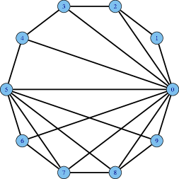
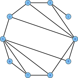
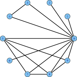
(a) $N$	(b) $N_{\textrm{min}}$	(c) $N_{\textrm{max}}$

Figure 3: (a) The ground truth network, (b) the network $N_{\textrm{min}}$ with minimal Ipsen-Mikhailov distance and (c) the network $N_{\textrm{max}}$ with maximal distance from the ground truth.

Both these experiments support the claim that Ipsen-Mikhailov metric has an higher resolution in discriminating between network structures.

4 APPLICATIONS

Evolution of dynamic networks

In (Kolar et al., 2010), the authors used the Keller algorithm to infer the gene regulatory networks of Drosophila melanogaster from a time series of gene expression data measured during its full life cycle. They selected 66 time points during the developmental cycle, spanning across four different stages (Embryonic – time points 1-30, Larval – t.p. 31-40, Pupal – t.p. 41-58, Adult – t.p. 59-66), following the dynamics of 588 gene ontological groups and then constructing a time series of inferred networks $N_{i}$. Hereafter we evaluate the structural differences between $N_{i}$ and $N_{i+1}$ and the distance between $N_{i}$ and the initial network $N_{1}$, measured either by the Ipsen-Mikhailov distance or by MCC: the resulting plots are displayed in Fig. 4.

(a) $\epsilon(N_{i},N_{i+1})$	(b) $\epsilon(N_{i},N_{1})$
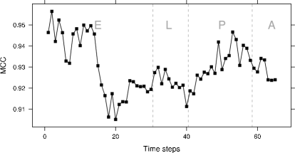
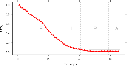
(c) $MCC(N_{i},N_{i+1})$	(d) $MCC(N_{i},N_{1})$
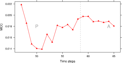
	(e) $MCC(N_{i\geq 47},N_{1})$

Figure 4: $\epsilon$ and MCC distances computed on consecutive elements (a and c) and with respect to the first element of the series (b and d) of the dynamic transcriptional network on 66 time points of the developmental cycle of D. melanogaster; in (e), zoom of (d) on the time points 47-65.

The largest variations, both between consecutive terms and with respect to the initial network $N_{1}$, occur in the embrional stage (E). As expected, the variations between consecutive terms (panels (a) and (c)) are smaller, while more relevant changes occur comparing a term with $N_{1}$. In particular, it is interesting to note that the dynamics of the networks move $N_{i}$ away from $N_{1}$ until time points 20, then the following terms start getting closer again to $N_{1}$ in terms of Ipsen-Mikhailov distance. The same trend is captured by MCC, but with lower resolution: the fact that MCC curve is ascending from its minimum in the last 15 time points can be appreciated only by zooming in from panel (d) to panel (e). This means that, after the embrional stage, the network is getting structurally more and more similar again to $N_{1}$, but with a limited number of links matching those of $N_{1}$.

Networks in profiling tasks

In the papers (Budhu et al., 2008; Ji et al., 2009), the authors introduced and analyzed a dataset collecting 482 tissue samples from 241 patients affected by hepatocellular carcinoma (HCC). For each patients, a sample from cancerous hepatic tissue and a sample from surrounding non-cancerous hepatic tissue have been hybridized on the Ohio State University CCC MicroRNA Microarray Version 2.0 platform consisting of 11520 probes collecting expressions of 250 non-redundant human and 200 mouse microRNA (miRNA).

Table 1: Workflow of the machine learning pipeline for the profiling tasks on the $\mathcal{HCC}$ dataset.

1. Preprocessing phase: imputation of missing values (Troyanskaya et al., 2001) and discarding probes corresponding to non-human (mouse and controls) miRNA;

2. Obtaining a dataset $\mathcal{HCC}$ of 240+240 paired samples described by 210 human miRNA

3. Three profiling experiments: discriminate the two classes Tumoral (T) and non Tumoral (nT) within the whole set $\mathcal{HCC}$, in the subset $\mathcal{HCC}_{M}$ of the 210+210 samples belonging to male patients (M) and in the subset $\mathcal{HCC}_{F}$ of the 30+30 samples belonging to female (F) patients;

4. Data Analysis Protocol (DAP) as in (Budhu et al., 2008): 1000 $\times$ 10-fold Cross Validation;

5. Classifier: Spectral Regression Discriminant Analysis (SRDA) (Cai et al., 2008), $\alpha=100$, Feature Ranking: Entropy-based Recursive Feature Elimination (E-RFE) (Furlanello et al., 2003);

6. Performance: MCC averaged on the 1000 test set for models with different number of features; confidence intervals are computed as 95% student bootstrap;

7. Ranked list Stability: the Canberra stability indicator $I$ (Jurman et al., 2008) defined as the mean of mutual Canberra distances among the lists, normalized with respect to the whole set of possible permutations. The smaller the indicator value, the higher the stability level of the lists, with 0 corresponding to a set of 10000 identical lists and 1 to a set of randomly ranked lists;

8. Results: The model with 20 features is a reasonable compromise between classifier performance, list stability and small number of features: for the tasks with all samples, $MCC=0.845$ $CI=(0.839,0.850)$, $I=0.166$, while for the other two cases the analogous values are $M=(0.931,(0.927,0.934),0.323)$ and $F=(0.859,(0.846,0.871),0.349)$;

9. Optimal list: for each of the three problems is computed as the top-20 sublist of the whole Borda list (Jurman et al., 2008; Borda, 1781);

10. In Tab. 2 we list the 16 miRNA common to at least two out of the three top-20 models: in particular, 7 miRNA are common to all the three problems.

By the Machine Learning pipeline detailed in Tab. 1 we extract the top-20 optimal set of features discriminating cancer samples from controls. Most of them are already known in literature as associated with hepatocellular carcinoma.

Table 2: Common miRNA

$\mathcal{HCC}$	hsa-mir-021-prec-17No1	hsa-mir-099-prec-21
	hsa-mir-128b-precNo1	hsa-mir-21No1
$\mathcal{HCC}_{M,F}$	hsa-mir-221-prec	hsa-mir-222-precNo1
	hsa-mir-26a-1No2
$\mathcal{HCC}$	hsa-mir-122a-prec
$\mathcal{HCC}_{M}$
$\mathcal{HCC}$	hsa-mir-100No1	hsa-mir-125b-1
	hsa-mir-199b-precNo2
$\mathcal{HCC}_{F}$	hsa-mir-219-1No2	hsa-mir-222-precNo2
$\mathcal{HCC}_{M}$	hsa-mir-130a-precNo2
$\mathcal{HCC}_{F}$	hsa-mir-146-prec

The following phase consists in the construction of the six weighted miRNA networks associated to the data subsets MT, MnT, FT, FnT, (M+F)T, (M+F)nT by using three different inference algorithm: WGCNA (Zhang and Horvath, 2005; Zhao et al., 2010; Horvath, 2011), Aracne (Margolin et al., 2006) and CLR (Faith et al., 2007), also considering their binarized versions after thresholding. As an example, in Fig. 5 we show the correlation networks at threshold $0.85$ in all the six considered cases: the number of links in the healthy tissue case is always larger than in the cancerous tissue case.

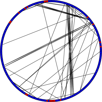
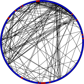
(a) (M+F) T		(b) (M+F) nT
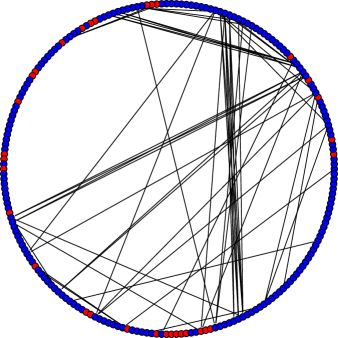
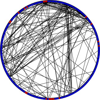
(c) M T		(d) M nT
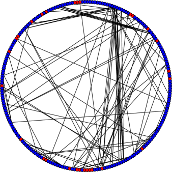
(e) F T		(f) F nT

Figure 5: Relevance network at correlation 0.85 for (left) the tumoral samples (T) and (right) the control tissues (nT), for the whole dataset (M+F), the male patients (M) and the female patients (F), with the top-20 ranked features marked as red nodes.

Using Ipsen-Mikhailov distance, it is now possibile to quantitatively explore the similarity among the miRNA profile networks: in what follows, we show some examples.

For instance, in Fig. 6 we show how distances between four couples of correlation networks evolve with the correlation threshold travelling between 0.1 and 0.9. The two closest networks are those corresponding to the Control tissues, with a classwise related trend independent from gender. In fact, the two curves expressing respectively the distance in the Tumorous tissue case between Male and Female patients and the corresponding curve for the Control tissue have a similar shape up to correlation threshold 0.8. Finally, for Female patients, the Tumoral network is quite distant from the Control one, hilighting a wider biological transformation caused by the disease than in Male patients.

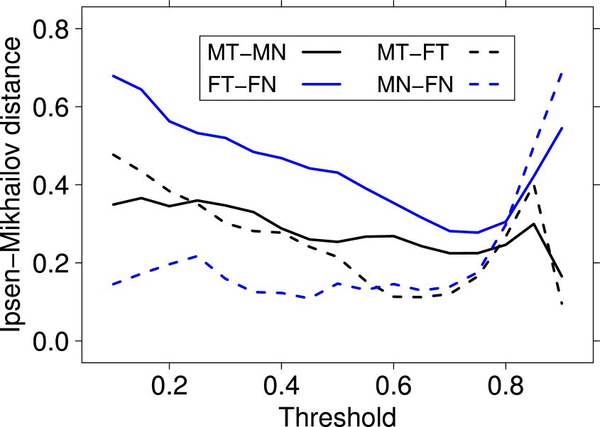
Figure 6: Evolutions of distances between 4 couples of correlation networks as a function of the correlation threshold.

In Tab. 3 the Ipsen-Mikhailov distances are reported among all six weighted networks for different methods, either on the whole set of 210 miRNA or on the top-20 set of optimal features. The corresponding multidimensional scaling projections are displayed in Fig. 7.

Table 3: Ipsen-Mikhailov distances among all six networks for different inference methods, on the whole set of 210 miRNA (upper triangular) or on the top-20 set of optimal features (lower triangular).

Mutual distances for weighted WGCNA networks
	F T	M T	M+F T	F nT	M nT	M+F nT
F T		0.1440	0.1228	0.3538	0.3056	0.2929
M T	0.4091		0.0838	0.3498	0.2845	0.2742
M+F T	0.3996	0.1091		0.3587	0.3012	0.2871
F nT	0.7648	0.5980	0.6272		0.1659	0.1634
M nT	0.5998	0.3687	0.4176	0.4403		0.0500
M+F nT	0.6197	0.3962	0.4389	0.4344	0.0594
Mutual distances for weighted Aracne networks
	F T	M T	M+F T	F nT	M nT	M+F nT
F T		0.1764	0.1636	0.1219	0.1210	0.1179
M T	0.3162		0.0408	0.2358	0.1132	0.1299
M+F T	0.3237	0.1241		0.2280	0.1075	0.1271
F nT	0.3604	0.4183	0.4400		0.1685	0.1658
M nT	0.2934	0.2454	0.2926	0.2344		0.0570
M+F nT	0.2945	0.2960	0.3370	0.2120	0.1194
Mutual distances for weighted CLR networks
	F T	M T	M+F T	F nT	M nT	M+F nT
F T		0.0043	0.0037	0.0056	0.1194	0.1233
M T	0.3260		0.0008	0.0030	0.1158	0.1102
M+F T	0.2441	0.2506		0.0028	0.1123	0.1067
F nT	0.4223	0.3571	0.3788		0.0964	0.0017
M nT	0.3380	0.3669	0.3160	0.3235		0.0011
M+F nT	0.3318	0.3577	0.3012	0.3251

The distances among networks show that there are substantial differences not only between the Tumorous/NonTumorous tissue samples, but also between Male and Female patients, both on the cancerous and the surrounding healthy tissue relevance networks. In particular, it can be pointed out that the networks corresponding to the tumoral tissue for female patients has a deeply different structure with respect to all other networks, while the differences between the models on all patients and those on the sole male population are smaller. This may be an effect of the different numerosity between male and female patients (210 versus 30) for WGCNA networks, but it is confirmed also by the Aracne algorithm which is less sensible to sample size differences. Finally, CLR is the algorithm where the difference between the networks built on the whole set of features and those built on the top-20 subset are more relevant.

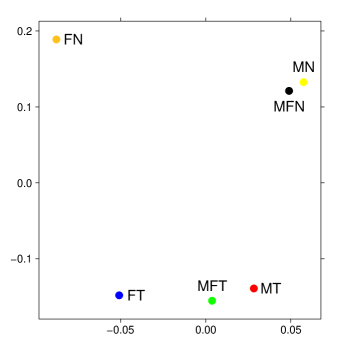
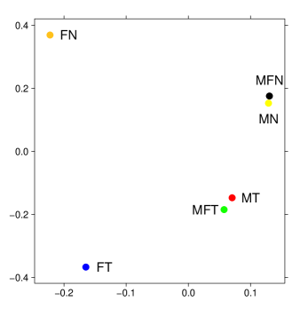
Weighted WGCNA networks
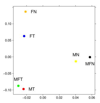
Weighted Aracne networks
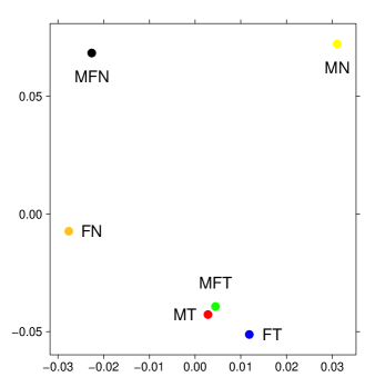
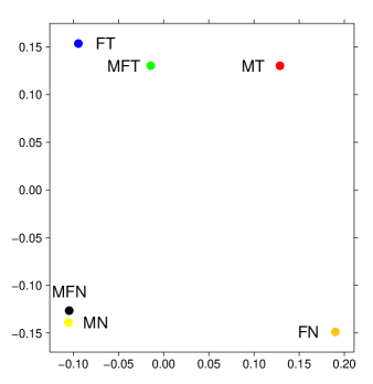
Weighted CLR networks

Figure 7: Multidimensional scaling of the distances listed in Tab. 3, for the complete set of miRNA (left panels) and the top-20 subset (right panels).

We can conclude with an analysis of distances across inference methods for networks associated to a given sample subset, listed in Tab. 4. The structures inferred by WGCNA and CLR are the closest when the full set of features are used, but distances are small among methods. The situation radically changes when the subset of optimal features is considered: in this case, WGCNA and Aracne tend to build up very similar networks for all the sample subsets, while CLR is going astray, confirming the observations drawn from the multidimensional scaling plots of Fig. 7.

Table 4: Ipsen-Mikhailov distances between weighted network inferred from the same sample subsets, for different inference methods WGCNA (W), Aracne (A) and CLR (C), for the whole set of miRNA (upper half) and the optimal top-20 miRNA subset (lower half).

Full set of 210 miRNA
	W,A	W,C	A,C
F T	0.6693	0.5732	0.7164
M T	0.6860	0.5648	0.7176
MF T	0.6831	0.5637	0.7207
F nT	0.6821	0.5289	0.7012
M nT	0.6678	0.5360	0.7011
M+F nT	0.6650	0.5337	0.6998
Optimal subset of 20 miRNA
	W,A	W,C	A,C
F T	0.2537	0.9567	0.9365
M T	0.3557	0.8320	0.8984
M+F T	0.3807	0.8343	0.9103
F nT	0.5192	0.8335	0.8625
M nT	0.3707	0.8198	0.8562
M+F nT	0.3628	0.8192	0.8555

Subset stability in network reconstruction

In this last example, we want to assess the stability of a network inferred by high-throughput data in terms of distances between networks generated from data subsampling. Sources of variability in this context are several: as a case study, here we consider three different publicly available (on GEO) microarray studies on the same pathology (colorectal cancer), on the same array platform (Affymetrix Human Genome U133 Plus 2.0 Array), with the same inference algorithm (WGCNA). References and details on the three datasets are listed in Tab. 5. The 33-genes signature from the paper (Smith et al., 2010) (developed for differentiating Dukes’ stage A and D and tested on stages B and C) are selected as the vertices of the subnetwork to infer.

Table 5: Size of patient cohorts grouped by disease stage

	Reference and GEO Accession Number
	(Jorissen et al., 2009)	(Kaiser et al., 2007)	(Smith et al., 2010)
Dukes/AJCC Stage	GSE14333	GSE5206	GSE17536/GSE17538
A/I	44	12	28
B/II	94	32	72
C/II	91	33	76
D/IV	61	21	56

The 33 genes map on 85 probes of the platform; during analysis, the expression of a gene is computed by averaging samplewise the expressions of all its mapping probes. The list of the 33 genes included in the signature, together with the mapped probes, is included in Tab. 6.

Table 6: The 33-gene CRC signature described in (Smith et al., 2010), with the mapped probes on the Affymetrix Human Genome U133 Plus 2.0 Array platform.

#	Gene name	Ensemble ID	Mapped probes
1	ACTB	ENSG00000075624	200801_x_at 213867_x_at 224594_x_at AFFX-HSAC07/X00351_3_at
			AFFX-HSAC07/X00351_5_at AFFX-HSAC07/X00351_M_at
2	DFNB31	ENSG00000095397	221887_s_at 47553_at
3	TMEM14A	ENSG00000096092	218477_at
4	CIRBP	ENSG00000099622	200810_s_at 200811_at 225191_at 228519_x_at 230142_s_at
5	SYT17	ENSG00000103528	205613_at 229053_at
6	AK1	ENSG00000106992	202587_s_at 202588_at
7	MGP	ENSG00000111341	202291_s_at 238481_at
8	VDR	ENSG00000111424	204253_s_at 204254_s_at 204255_s_at 213692_s_at
9	C6orf64	ENSG00000112167	218784_s_at 222741_s_at 232992_at
10	HES1	ENSG00000114315	203393_at 203394_s_at 203395_s_at
11	TEX11	ENSG00000120498	221259_s_at 233514_x_at 234296_s_at
12	MYOT	ENSG00000120729	219728_at
13	EGR1	ENSG00000120738	201693_s_at 201694_s_at 227404_s_at
14	DCTD	ENSG00000129187	201571_s_at 201572_x_at 210137_s_at
15	MMP13	ENSG00000137745	205959_at
16	TACC2	ENSG00000138162	1570025_at 1570546_a_at 202289_s_at 211382_s_at
17	CXCR7	ENSG00000144476	1559114_a_at 212977_at 232746_at
18	DENND2A	ENSG00000146966	221885_at 221886_at 53991_at
19	MUM1L1	ENSG00000157502	229160_at
20	PDLIM5	ENSG00000163110	203242_s_at 203243_s_at 211680_at 211681_s_at 212412_at
			213684_s_at 216803_at 216804_s_at 221994_at 241208_at
21	SPDYA	ENSG00000163806	238262_at
22	NMNAT3	ENSG00000163864	228090_at 243738_at
23	CRABP1	ENSG00000166426	1563897_at 205350_at
24	ACYP2	ENSG00000170634	206833_s_at
25	CSN3	ENSG00000171209	207803_s_at
26	HPSE	ENSG00000173083	219403_s_at 222881_at
27	STOX2	ENSG00000173320	226822_at 231969_at 234317_s_at 234319_at
28	SLC25A30	ENSG00000174032	226782_at 238171_at
29	NQO1	ENSG00000181019	201467_s_at 201468_s_at 210519_s_at
30	SPRY4	ENSG00000187678	220983_s_at 221489_s_at
31	S100A3	ENSG00000188015	206027_at
32	PRTN3	ENSG00000196415	207341_at
33	HS3ST5	ENSG00000249853	240479_at

In Fig. 8 we show as an example three of the coexpression graphs (on the whole set of data) for stages C and D for three different datasets. The node numbering is taken from Tab. 6, the node size is proportional to its degree and the edge width is proportional to its weight.

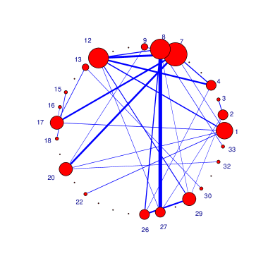
(a)	(b)
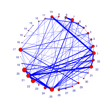
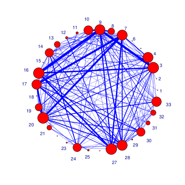
(c)	(d)

Figure 8: Examples of topology of weighted coexpression networks: (a) GSE14333, Stage C (b) GSE14333, Stage D (c) GSE5206, Stage C (c) 17536/8, Stage C. Node numbering inherited from Tab. 6, node size and edge width proportional to degree and weight respectively.

To quantify network stability, for a given dataset and stage, we select a random fraction $p$ of the data and we generate the corresponding WGCNA; this procedure is repeated $N$ times, so to end up with $N$ WGCNA for each configuration (dataset, stage and $p$). Then all mutual $\binom{N}{2}=\frac{N(N-1)}{2}$ Ipsen-Mikhailov distances are computed, and for each set of $N$ graphs we build the corresponding distance histogram, reporting also mean and standard deviation. The lower the mean and the variance, the stabler the inferred network.

In Tab. 7 we show the results for $p=\frac{1}{2}$ and $p=\frac{2}{3}$, with $N=100$ replicates.

Table 7: Mean and variance for the sets of 4950 distances for all combinations of dataset and stage, in the two cases of using 2/3 and 1/2 of the data.

$p=\frac{2}{3}$	Stage A		Stage B		Stage C		Stage D
	$\mu$	$\sigma^{2}$	$\mu$	$\sigma^{2}$	$\mu$	$\sigma^{2}$	$\mu$	$\sigma^{2}$
GSE14333	0.1988	0.0065	0.1787	0.0088	0.1843	0.0086	0.2447	0.0112
GSE5206	0.2457	0.0073	0.2180	0.0051	0.2777	0.0137	0.2409	0.0086
GSE17536/8	0.3306	0.0169	0.2301	0.0040	0.2199	0.0028	0.2173	0.0038
$p=\frac{1}{2}$	Stage A		Stage B		Stage C		Stage D
	$\mu$	$\sigma^{2}$	$\mu$	$\sigma^{2}$	$\mu$	$\sigma^{2}$	$\mu$	$\sigma^{2}$
GSE14333	0.2075	0.0066	0.2135	0.0112	0.2028	0.0104	0.2978	0.0159
GSE5206	0.2602	0.0070	0.2464	0.0071	0.2931	0.0146	0.2596	0.0095
GSE17536/8	0.3668	0.0176	0.2681	0.0048	0.2646	0.0044	0.2483	0.0061

For stages A, B and C the best stability is detected on the GSE14333 dataset, while for stage D GSE175536/8 results the stabler dataset. Moreover, the $(\mu,\sigma^{2})$ couples listed in Tab. 7 do not show a great variability among the 24 listed cases. A larger range of situations can be appreciated by looking at the shapes of the distribution of each set of 4950 distances. In fact, although some of the cases are almost gaussian-like, a number of other combinations of dataset and stage are represented by very skewed distribution: for them, considering mean and variance as descriptive parameters may be interpretatively misleading. As an example, GSE14333, Stage D and GSE17536/8, Stage B for $p=\frac{2}{3}$ have rather similar mean and variance, but a quite different distribution shape as shown by Fig. 9).

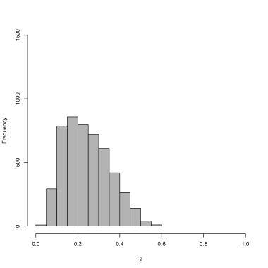
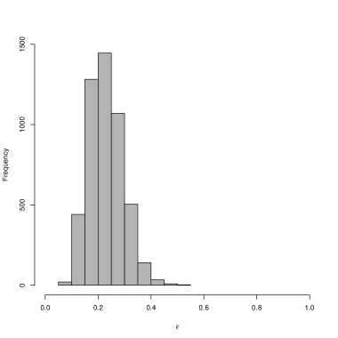
(a)	(b)
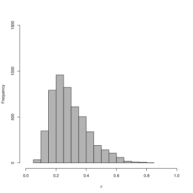
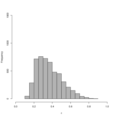
(c)	(d)

Figure 9: Histogram of distance distributions for four of the cases listed in Tab. 7: (a) GSE14333, Stage D, $p=\frac{2}{3}$, (b) GSE17536/8, Stage B, $p=\frac{2}{3}$, (c) GSE5206, Stage C, $p=\frac{2}{3}$, (d) GSE17536/8, Stage A, $p=\frac{1}{2}$.

We can conclude observing that the plotted histograms show how in several cases the infered network can be heavily dependent on the particular chosen subset of data, leaving the network built on the whole dataset affected by a relatively large level of uncertainty (instability): this may be due both to high variability in the data distribution, but also to high sensibility of the algorithm to data perturbation. This fact should always be taken into account when assessing the reliability of a reconstructed network in order to avoid drawing biological consideration from a possible false positive edge linking two nodes.

5 DISCUSSION

Ipsen-Mikhailov $\epsilon$ distance is an effective metric for comparing (biological) networks in various situations. Its definition involves the distribution of the Laplacian spectrum of the networks, so it deal with the structure of the underlying graph, rather than focussing on the local pattern of the wiring differences. It is mostly consistent with more classification measures such as MCC, but it allows detection of finer differences. The presented examples show effectiveness and usefulness of $\epsilon$ in different biological tasks, but additional applications can be considered wherever a quantitative network comparison is needed. Finally, the use of Ipsen-Mikhailov distance in Transcription Starting Sites network will be presented within the Fantom5 initiative led by Riken Institute.

DISCLOSURE STATEMENT

No competing financial interests exist.

References

- Almendral and Díaz-Guilera (2007) Almendral, J. and Díaz-Guilera, A., 2007. Dynamical and spectral properties of complex networks. New J. Phys. 9, 187.
- Atay et al. (2006) Atay, F., Bıyıkoğlu, T., and Jost, J., 2006. Network synchronization: Spectral versus statistical properties. Physica D Nonlinear Phenomena 224, 35–41.
- Baldi et al. (2000) Baldi, P., Brunak, S., Chauvin, Y., Andersen, C., and Nielsen, H., 2000. Assessing the accuracy of prediction algorithms for classification: an overview. Bioinformatics 16, 412–424.
- Banerjee and Jost (2009) Banerjee, A. and Jost, J., 2009. Graph spectra as a systematic tool in computational biology. Discrete Appl. Math. 157, 2425–2431.
- Barabasi et al. (2011) Barabasi, A.-L., Gulbahce, N., and Loscalzo, J., 2011. Network medicine: a network-based approach to human disease. Nature Reviews Genetics 12, 56–68.
- Barla et al. (2011) Barla, A., Jurman, G., Visintainer, R., Squillario, M., Filosi, M., Riccadonna, S., and Furlanello, C., 2011. A machine learning pipeline for discriminant pathways identification. In Proc. CIBB 2011 (in press).
- Belykh et al. (2005) Belykh, I., Hasler, M., Lauret, M., and Nijmeijer, H., 2005. Synchronization and graph topology. International Journal of Bifurcation and Chaos 15, 3423–3433.
- Borda (1781) Borda, J., 1781. Mémoire sur les élections au scrutin. Histoire de l’Académie Royale des Sciences Année MDCCLXXXI.
- Buchanan et al. (2010) Buchanan, M., Caldarelli, G., De Los Rios, P., Rao, F., and Vendruscolo, M., eds., 2010. Networks in Cell Biology. Cambridge University Press.
- Budhu et al. (2008) Budhu, A., Jia, H.-L., Forgues, M., Liu, C.-G., Goldstein, D., Lam, A., Zanetti, K. A., Ye, Q.-H., Qin, L.-X., Croce, C. M., Tang, Z.-Y., and Wang, X. W., 2008. Identification of Metastasis-Related MicroRNAs in Hepatocellular Carcinoma. Hepatology 47, 897–907.
- Bunke (2000) Bunke, H., 2000. Graph Matching: Theoretical Foundations, Algorithms, and Applications. In Proceedings of International Conference on Vision Interface, 82–88. IEEE.
- Cai et al. (2008) Cai, D., He, X., and Han, J., 2008. SRDA: An Efficient Algorithm for Large-Scale Discriminant Analysis. IEEE Transactions on Knowledge and Data Engineering 20, 1–12.
- Chung (1997) Chung, F., 1997. Spectral Graph Theory. American Mathematical Society.
- Faith et al. (2007) Faith, J., Hayete, B., Thaden, J., Mogno, I., Wierzbowski, J., Cottarel, G., Kasif, S., Collins, J., and Gardner, T., 2007. Large-Scale Mapping and Validation of Escherichia coli Transcriptional Regulation from a Compendium of Expression Profiles. PLoS Biol. 5, e8.
- Furlanello et al. (2003) Furlanello, C., Serafini, M., Merler, S., and Jurman, G., 2003. Entropy-Based Gene Ranking without Selection Bias for the Predictive Classification of Microarray Data. BMC Bioinformatics 4, 54.
- Haemers and Spence (2004) Haemers, W. and Spence, E., 2004. Enumeration of cospectral graphs. Eur. J. Comb. 25, 199–211.
- Horvath (2011) Horvath, S., 2011. Weighted Network Analysis: Applications in Genomics and Systems Biology. Springer.
- Ipsen and Mikhailov (2002) Ipsen, M. and Mikhailov, A., 2002. Evolutionary reconstruction of networks. Phys. Rev. E 66, 046109.
- Ji et al. (2009) Ji, J., Shi, J., Budhu, A., Yu, Z., Forgues, M., Roessler, S., Ambs, S., Chen, Y., Meltzer, P., Croce, C., Qin, L.-X., Man, K., Lo, C.-M., Lee, J., Ng, I., Fan, J., Tang, Z.-Y., Sun, H.-C., and Wang, X., 2009. MicroRNA Expression, Survival, and Response to Interferon in Liver Cancer. N. Engl. J. Med. 361, 1437–1447.
- Jorissen et al. (2009) Jorissen, R., Gibbs, P., Christie, M., Prakash, S., Lipton, L., Desai, J., Kerr, D., Aaltonen, L., Arango, D., Kruhøffer, M., Orntoft, T., Andersen, C., Gruidl, M., Kamath, V., Eschrich, S., Yeatman, T., and Sieber, O., 2009. Metastasis-Associated Gene Expression Changes Predict Poor Outcomes in Patients with Dukes Stage B and C Colorectal Cancer. Clinical Cancer Research 15, 7642–7651.
- Jost (2007) Jost, J., 2007. Dynamical Networks. In Feng, J., Jost, J., and Qian, M., eds., Networks: From Biology to Theory, 35–64. Springer-Verlag.
- Jost and Joy (2002) Jost, J. and Joy, M., 2002. Evolving Networks with distance preferences. Phys. Rev. E 66, 036126.
- Jurman et al. (2008) Jurman, G., Merler, S., Barla, A., Paoli, S., Galea, A., and Furlanello, C., 2008. Algebraic stability indicators for ranked lists in molecular profiling. Bioinformatics 24, 258–264.
- Jurman et al. (2011) Jurman, G., Visintainer, R., and Furlanello, C., 2011. An introduction to spectral distances in networks. Frontiers in Artificial Intelligence and Applications 226, 227–234.
- Kaiser et al. (2007) Kaiser, S., Park, Y.-K., Franklin, J., Halberg, R., Yu, M., Jessen, W., Freudenberg, J., Chen, X., Haigis, K., Jegga, A., Kong, S., Sakthivel, B., Xu, H., Reichling, T., Azhar, M., Boivin, G., Roberts, R., Bissahoyo, A., Gonzales, F., Bloom, G., Eschrich, S., Carter, S., Aronow, J., Kleimeyer, J., Kleimeyer, M., Ramaswamy, V., Settle, S., Boone, B., Levy, S., and Graff, J., 2007. Transcriptional recapitulation and subversion of embryonic colon development by mouse colon tumor models and human colon cancer. Genome Biology 8, R131.
- Kolar et al. (2010) Kolar, M., Song, L., Ahmed, A., and Xing, E., 2010. Estimating time-varying networks. Ann. Appl. Stat. 4, 94–123.
- Margolin et al. (2006) Margolin, A., Nemenman, I., Basso, K., Wiggins, C., Stolovitzky, G., Dalla-Favera, R., and Califano, A., 2006. ARACNE: an algorithm for the reconstruction of gene regulatory networks in a mammalian cellular context. BMC Bioinform. 7, S7.
- Matthews (1975) Matthews, B., 1975. Comparison of the predicted and observed secondary structure of T4 phage lysozyme. Biochimica et Biophysica Acta - Protein Structure 405, 442–451.
- Pavlopoulos et al. (2011) Pavlopoulos, G., Secrier, M., Moschopoulos, C., Soldatos, T., Kossida, S., Aerts, J., Schneider, R., and Bagos, P., 2011. Using graph theory to analyze biological networks. BioData Mining 4, 10.
- Rodgers et al. (2005) Rodgers, G., Austin, K., Kahng, B., and Kim, D., 2005. Eigenvalue spectra of complex networks. Journal of Physics A: Mathematical and General 38, 9431.
- Smith et al. (2010) Smith, J., Deane, N., Wu, F., Merchant, N., Zhang, B., Jiang, A., Lu, P., Johnson, J., Schmidt, C., Bailey, C., Eschrich, S., Kis, C., Levy, S., Washington, M., Heslin, M., Coffey, R., Yeatman, T., Shyr, Y., and Beauchamp, R., 2010. Experimentally Derived Metastasis Gene Expression Profile Predicts Recurrence and Death in Patients With Colon Cancer. Gastroenterology 138, 958–968.
- Spielman (2009) Spielman, D., 2009. Spectral Graph Theory: The Laplacian (Lecture 2). Lecture notes.
- Stokic et al. (2009) Stokic, D., Hanel, R., and Thurner, S., 2009. A fast and efficient gene-network reconstruction method from multiple over-expression experiments. BMC Bioinformatics 10, 253.
- Supper et al. (2007) Supper, J., Spieth, C., and Zell, A., 2007. Reconstructing Linear Gene Regulatory Networks. In Marchiori, E., Moore, J., and Rajapakse, J., eds., Proceedings of the 5th European Conference on Evolutionary Computation, Machine Learning and Data Mining in Bioinformatics, EvoBIO2007, LNCS 4447, 270–279. Springer-Verlag.
- The MicroArray Quality Control Consortium(2010) (MAQC) The MicroArray Quality Control (MAQC) Consortium, 2010. The MAQC-II Project: A comprehensive study of common practices for the development and validation of microarray-based predictive models. Nat. Biotechnol. 28, 827–838.
- Tönjes and Blasius (2009) Tönjes, R. and Blasius, B., 2009. Perturbation Analysis of Complete Synchronization in Networks of Phase Oscillators. ArXiv:0908.3365.
- Troyanskaya et al. (2001) Troyanskaya, O., Cantor, M., Sherlock, G., Brown, P., Hastie, T., Tibshirani, R., Botstein, D., and Altman, R., 2001. Missing value estimation methods for DNA microarrays. Bioinformatics 17, 520–525.
- Vidal et al. (2011) Vidal, M., Cusick, M.-E., and Barabasi, A.-L., 2011. Interactome Networks and Human Disease. Cell 144, 986–995.
- Wu et al. (2008) Wu, Y., Shang, Y., Chen, M., Zhou, C., and Kurths, J., 2008. Synchronization in small-world networks. Chaos 18, 037111.
- Zhang and Horvath (2005) Zhang, B. and Horvath, S., 2005. A General Framework for Weighted Gene Co-Expression Network Analysis. Statistical Applications in Genetics and Molecular Biology 4, Article 17.
- Zhao et al. (2010) Zhao, W., Langfelder, P., Fuller, T., Dong, J., Li, A., and Hovarth, S., 2010. Weighted gene coexpression network analysis: state of the art. Journal of Biopharmaceutical Statistics 20, 281–300.