Studying Flow Close to an Interface by Total Internal Reflection
Fluorescence Cross Correlation Spectroscopy:
Quantitative Data Analysis

Abstract

Total Internal Reflection Fluorescence Cross Correlation Spectroscopy (TIR-FCCS) has recently (S. Yordanov et al., Optics Express 17, 21149 (2009)) been established as an experimental method to probe hydrodynamic flows near surfaces, on length scales of tens of nanometers. Its main advantage is that fluorescence only occurs for tracer particles close to the surface, thus resulting in high sensitivity. However, the measured correlation functions only provide rather indirect information about the flow parameters of interest, such as the shear rate and the slip length. In the present paper, we show how to combine detailed and fairly realistic theoretical modeling of the phenomena by Brownian Dynamics simulations with accurate measurements of the correlation functions, in order to establish a quantitative method to retrieve the flow properties from the experiments. Firstly, Brownian Dynamics is used to sample highly accurate correlation functions for a fixed set of model parameters. Secondly, these parameters are varied systematically by means of an importance-sampling Monte Carlo procedure in order to fit the experiments. This provides the optimum parameter values together with their statistical error bars. The approach is well suited for massively parallel computers, which allows us to do the data analysis within moderate computing times. The method is applied to flow near a hydrophilic surface, where the slip length is observed to be smaller than $10nm$, and, within the limitations of the experiments and the model, indistinguishable from zero.

I Introduction

A good understanding of liquid flow in confined geometries is not only of fundamental interest, but also important for a number of industrial and technological processes, such as flow in porous media, electro-osmotic flow, particle aggregation or sedimentation, extrusion and lubrication. It is also essential for the design of micro- and nano-fluidic devices, e. g. in lab-on-a-chip applications. However, in all these cases, an accurate quantitative description is only possible if the flow at the interface between the liquid and the solid is thoroughly understood Tabeling06 ; Vinogradova1999 ; Ellis04 ; Net05 ; Lauga07 ; Bonaccurso02 ; Neto03 ; Rod10 ; Guriyanova08 ; Feuillebois09 . While for many years the so-called no-slip boundary condition (relative velocity at the interface equal to zero) had been successfully applied to describe macroscopic flows, more recent investigations revealed that this condition is insufficient to describe the physics when flows through channels with micro- and nano-sizes are considered Net05 ; Lauga07 . On such small scales, the relative contribution from a residual slip between liquid and solid becomes important. This is commonly described by the so-called slip boundary condition, which is characterized by a non-vanishing slip length $l_{s}$, defined as the ratio of the liquid dynamic viscosity and the friction coefficient per unit area at the surface. An equivalent definition is obtained by taking the ratio of the finite surface flow velocity, the so-called slip velocity $v_{s}$, and the shear rate at the surface: $l_{s}=v_{s}/(dv/dz)_{z=0}$, where $z$ is the spatial direction perpendicular to the surface, located at $z=0$. This boundary condition is the most general one that is possible within the framework of standard hydrodynamics einzel1990boundary ; the no-slip condition is simply the special case $l_{s}=0$.

The experimental determination of the slip length, however, is challenging, since high resolution techniques are needed to gain sufficiently accurate information close to the interface. Hence, the existence and the magnitude of slip in real physical systems, as well as its possible dependence on the surface properties, are highly debated in the community, and no consensus has been reached so far. Clearly, a resolution of these controversies requires further improvement of the experimental techniques.

To date, two major types of experimental methods, often called direct and indirect, have been applied to study boundary slip phenomena. In the indirect approach, an atomic force microscope or a surface force apparatus is used to record the hydrodynamic drainage force necessary to push a micron-sized colloidal particle versus a flat surface as a function of their separation Ducker1991 ; Butt1991 . The separation can be measured with sub-nanometric resolution, and the force with a resolution in the $pN$ range. A high force is necessary to squeeze the liquid out of the gap if the mobility of the liquid is small. Conversely, if the liquid close to the surface can easily slip on it, then a small force is necessary. From this empirical observation a quantitative value of the slip length can be deduced using an appropriate theoretical model Vinogradova1999 ; Vinogradova1995 ; Bonaccurso02 . While this approach is extremely accurate at the nanoscale, it does not measure the flow profile directly.

Direct experimental approaches to flow profiling in microchannels are commonly based on various optical methods to monitor fluorescent tracers moving with the liquid. Basically they can be divided into two sub-categories.

The imaging-based methods use high-resolution optical microscopes and sensitive cameras to track the movement of individual tracer particles via a series of images Pit2000 ; Tretheway02 ; Jos05 ; Huang06 ; Lasne08 ; Bouzigues08 ; Li10 . While providing a real “picture” of the flow, the imaging methods have also some disadvantages related mainly to the limited speed and sensitivity of the cameras: relatively big tracers are needed, the statistics is rather poor, and large tracer velocities cannot be easily measured.

In the Fluorescence Correlation Spectroscopy (FCS) based methods the fluctuations of the fluorescent light emitted by tracers passing through a small observation volume (typically the focus of a confocal microscope) are measured Rigler01 . Using correlation analysis and an appropriate mathematical model the tracers’ diffusion coefficient and flow velocity can be evaluated Magde1978 ; Orden1998 ; Kohler2000 ; Gosch2000 . In particular, the so-called Double-Focus Fluorescence Cross-Correlation Spectroscopy (DF-FCCS) that employs two observation volumes (laterally shifted in flow direction) is a powerful tool for flow profiling in microchannels Bri99 ; Dit02 ; Lum03 ; Vin09 . Due to the high sensitivity and speed of the used photo detectors (typically avalanche photodiodes) in the FCS based methods even single molecules can be used as tracers. Furthermore, the evaluation of the velocity is based on large statistics and high tracer velocities can be measured.

During the last two decades both the imaging and the FCS methods were well developed to the current state that allows fast and accurate measurements of flow velocity profiles in microchannels. The situation, however, is different when the issue of boundary slip is considered. Due to the limited optical resolution imposed by the diffraction limit, it is commonly believed that these methods are less accurate than the force methods discussed above and cannot detect a slip length in the tens of nanometers range. On the other hand, the possibility to directly visualize the flow makes the optical methods still attractive and thus continuous efforts were undertaken to improve their resolution. One of the most successful approaches in this endeavor is Total Internal Reflection Microscopy (TIRM) Axelrod1984 , which uses total internal reflection at the interface between two media with different refractive indices, like, e. g., glass and water. This creates an evanescent wave that extends into the liquid in a tunable region of less than $\sim 200nm$ from the interface. Optical excitation of the fluorescent tracers is then possible only within this narrow region. During the last few years TIRM was successfully applied to improve the resolution of particle imaging velocimetry close to liquid-solid interfaces Huang06 ; Lasne08 ; Bouzigues08 ; Li10 , and slip lengths in the order of tens of nanometers were evaluated. With respect to FCS, however, TIR illumination had, until recently, been limited to diffusion studies only HasslerSecond05 ; Rie08 , while there were no reports on TIR-FCS based velocimetry and slip length measurements.

With this in mind, we have recently developed a new experimental setup that combines for the first time TIR illumination with DF-FCCS for monitoring a liquid flow in the close proximity of a solid surface Koy09 . Such a combination offers high normal resolution, extreme sensitivity (down to single molecules), good statistics within relatively short measurement times and the possibility to study fast flows. Our preliminary studies have shown, however, that the accurate quantitative evaluation of the experimental data obtained with this TIR-FCCS setup is not straightforward because the model functions needed to fit the auto- and cross-correlation curves (and extract the flow velocity profile) are not readily available. The standard analytical procedure to derive these functions is Bri99 ; Dit02 ; Lum03 : (i) solve the convection-diffusion equation with respect to the concentration correlation function, (ii) insert the derived solution in the corresponding correlation integral and (iii) solve it to finally get the explicit form of the correlation functions. This procedure was successfully used by Brinkmeier et al. Bri99 to derive analytical expressions for the auto- and cross-correlation functions obtained with double focus confocal FCCS (i. e. with focused laser beam illumination as opposed to the evanescent wave illumination in our case), where it was assumed that the flow velocity and tracer concentration are spatially constant, which simplifies the calculation substantially. Such an assumption is reasonable if the observation volumes (laser foci) are far away from the channel walls, in the same distance. In the case of TIR-FCCS, however, the situation is different: The experiments are performed in the proximity of the channel wall and the distribution of the flow velocity inside the observation volume has to be considered. Furthermore, the concentration of tracers may also depend on $z$ due to electrostatic repulsion or hydrodynamic effects. Finally the presence of a boundary, which must also be taken into account in the theoretical treatment, further complicates the problem. Therefore, a faithful description of the physics of TIR-FCCS makes the problem of calculating the correlation functions (rather likely) unsolvable in terms of closed analytical expressions.

For this reason, we rather resort to numerical methods, and in the present paper describe and test the procedure that we have developed: We employ Brownian Dynamics techniques to simulate the tracers’ motion through the observation volumes and generate “numerical” auto- and cross-correlation curves that are consequently used to fit the corresponding experimental data. This fitting is done via Monte Carlo importance sampling in parameter space. The method is therefore fully quantitative, while not being hampered by any difficulties in doing analytical calculations. It should be noted that this approach also provides a substantial amount of flexibility: The details of the physical model are all encoded in the Brownian Dynamics simulation which specifies how the tracer particles move within the flow. In the present work we have assumed a simple Couette flow with a finite slip length, while the particles are described as simple hard spheres with no rotational degree of freedom, and no interaction with the wall except impenetrability. It is fairly straightforward to improve on these limitations, by, e. g., including hydrodynamic and electrostatic interactions with the wall, rotational motion of the spheres, or polydispersity in the particle size distribution. Moreover, the geometry of the observation volumes can be easily changed as well, and we have made use of this possibility in our present work, but only to some extent. Further refinements are left for future work, in which the basic methodology would however remain unchanged.

To test the accuracy of the newly developed TIR-FCCS experimental setup and the numerical data evaluation procedure, we have studied aqueous flow near a smooth hydrophilic surface and evaluated the slip length to be between $0$ and $10nm$ (however with a systematic error that is hard to quantify, and whose elimination would need a more sophisticated theoretical model). It is commonly accepted Lasne08 ; Bouzigues08 ; Li10 ; Idol1986 ; Jos05 ; Charlaix05 ; Joly06 ; Honig07 that the boundary slip should be zero (or very small) in this situation. Thus, our results indicate that TIR-FCCS offers unprecedented accuracy in the $10nm$ range for the measurement of slip lengths by an optical method. We believe that our result for the slip length will be fairly robust, even if the physical model is refined further.

Section II outlines the experimental setup, while Sec. III presents the experimental results and the numerical fits. We find that the measured cross-correlation functions deviate considerably from the model functions at short times, probably as a result of some optical effects which at present we do not fully understand. However, we show a practical way to eliminate such effects to a large extent, by means of a simple subtraction scheme. The following parts then outline in detail how the theoretical curves have been obtained: Firstly, Sec. IV elucidates the relation between the measured correlation functions and the underlying dynamics of the tracer particles. We then proceed to describe the Brownian Dynamics algorithm to sample the model correlation functions (Sec. V). Section VI then provides a detailed theoretical analysis of our subtraction scheme. In Sec. VII we describe the Monte Carlo method to find optimized parameter values of our model. Section VIII then discusses our results, in particular concerning the slip length; this is followed by a brief summary of our conclusions (Sec. IX).

II Experimental Setup

Figure 1: (Color) Scheme of the experimental TIR-FCCS setup. BFP - back focal plane of the objective; DM - dichroic mirror; M50/50 - neutral $50\%$ beam splitter; EF1, EF2 - emission filters; PH1, PH2 - pinholes; APD1, APD2 - avalanche photodiodes; L1 - tube lens; L2 - collimator lens; M - collimator’s prism based mirror. Note that the two spatially separated observation volumes are created by shifting the pinholes PH1/PH2 in the $x$-$y$-plane. The cyan color indicates the excitation wavelength and the yellow-green color the fluorescence light, respectively.

Since the TIR-FCCS experimental setup has already been described in great detail elsewhere Koy09 , only a brief qualitative overview of the basic ideas and quantities is given below. A scheme of the experimental setup is shown in Fig. 1. It is based on a commercial device (Carl Zeiss, Jena, Germany) that consists of the FCS module ConfoCor2 and an inverted microscope Axiovert 200. The TIR illumination is achieved by focusing the excitation laser beam ($488nm$, Ar⁺ Laser) on the periphery of the back focal plane (BFP) of an oil immersion microscope objective with numerical aperture $NA=1.46$. This leads to a parallel laser beam which emerges out of the objective and then enters the rectangular flow channel through its bottom wall (Fig. 1). By adjusting the angle of incidence above the critical angle ($\approx 61\degree$ for the glass-water interface) total internal reflection is achieved. In this situation only an evanescent wave extends into the liquid and can excite the fluorescent tracers suspended in it. The intensity distribution of this wave in the $x$-$y$-plane (parallel to the interface) is Gaussian with a diameter of $\sim 30\mu m$ (at $e^{-1}$). In the $z$ direction the intensity decays exponentially, $I(z)=I_{0}\exp(-z/d_{p})$. The characteristic decay length $d_{p}$, also called penetration depth, depends on the laser wavelength $\lambda$, the refraction indices of both media ($n_{1}$ - glass, $n_{2}$ - water) and can be varied in the range $80-200nm$ by changing the angle of incidence. Thus the evanescent wave can excite only the tracers flowing in the proximity of the channel wall. The produced fluorescence light is collected by the same microscope objective and is equally divided by passing through a neutral $50\%$ beam splitter to enter two independent detection channels. In each channel the fluorescent light passes through an emission filter and a confocal pinhole to finally reach the detectors, two single photon counting avalanche photodiodes (APD1, APD2). The pinholes PH1 and PH2 define two observation volumes that are laterally shifted with respect to each other along the flow direction as schematically shown in Fig. 2. The center-to-center distance $s_{x}$ between the two observation volumes can be continuously tuned from $0$ to $3\mu m$. The signals from both channels are recorded and correlated to finally yield the auto- and cross-correlation curves that contain the entire information about the flow properties, slip length and shear rate, close to the interface.

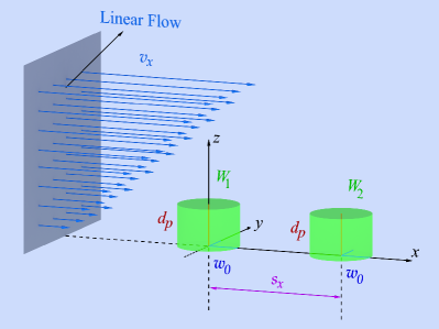
Figure 2: (Color) The coordinate system and the linear flow field employed in the TIR-FCCS experiment. $W_{1}$ and $W_{2}$ denote the shape and location of the observation volumes as seen by pinhole PH1 and pinhole PH2, respectively; $d_{p}$ is the penetration depth which defines the axial extent of the observation volume; $w_{0}$ is the typical extension of the observation volumes in the $x$-$y$-plane; $s_{x}$ indicates the observation volumes separation, center-to-center distance; $v_{x}$ is the velocity field in positive $x$ direction, which depends linearly on $z$.

The experiments were performed with a rectangular microchannel of $L_{y}=4mm$ width, $L_{z}=100\mu m$ height and $L_{x}=50mm$ length fabricated using a three-layer sandwich construction as described in earlier work Koy09 ; Lum03 . The bottom channel wall at which the TIR-FCCS experiments were performed was a microscope cover slide made of borosilicate glass with a thickness of $170\mu m$, cleaned with $2\%$ aqueous solution of Hellmanex and Argon plasma. The root-mean-square roughness of the glass surface was in the range of $0.3nm$ and the water advancing contact angle below $5\degree$ (hydrophilic surface). The flow was induced by a hydrostatic pressure gradient, created by two beakers of different heights, where the water level difference was kept constant by a pump. This allowed us to vary the shear rate near the wall in the range $0-5000s^{-1}$.

Carboxylate-modified quantum dots (Qdot585 ITK Carboxyl, Molecular Probes, Inc.), with a hydrodynamic radius $R_{H}=6.87nm$, were used as fluorescent tracers. The particles were suspended in an aqueous solution of potassium phosphate ($K_{2}HPO_{4}$) buffer ($pH\simeq 8.0$, concentration $6mM$). The concentration of the quantum dots was found from our data analysis (see below) as $\sim 30nM$, corresponding to roughly $18$ particles per $(\mu m)^{3}$.

III Correlation Curves

The motion of the fluorescence tracers results in two time-resolved fluorescence intensities $I_{1}(t)$ and $I_{2}(t)$, which were measured with the two photo detectors. For the present system, we may safely assume that it is ergodic and strictly stationary on the time scale of the experiment, such that only time differences matter Lakowicz06 . Therefore, we may define the intensity fluctuations via

$$\delta I_{i}(t)=I_{i}(t)-\langle I_{i}\rangle,$$ (1)

where $\langle\cdot\rangle$ denotes a time average or, equivalently, an ensemble average, and evaluate the time-dependent auto- and cross-correlation functions via the definition

$$G_{ij}(t)=\frac{\langle\delta I_{i}(0)\delta I_{j}(t)\rangle}{\langle I_{i}\rangle\langle I_{j}\rangle}.$$ (2)

It should be noted that possible small differences in the sensitivity of the photo detectors or in the illumination of the pinholes cancel out, since in Eq. 2 only ratios of intensities occur. $G_{11}$ and $G_{22}$ are the two autocorrelation functions of pinholes $1$ and $2$, respectively, while $G_{12}$ and $G_{21}$ are the forward and backward cross-correlation functions, respectively. It should be noted that in the presence of flow $G_{12}$ and $G_{21}$ differ substantially. In the limit of the two pinholes being located at the same position, the intensities $I_{1}$ and $I_{2}$ coincide, such that in this case all four entries of the matrix $G_{ij}$ are identical.

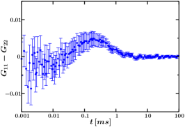
(a)	(b)
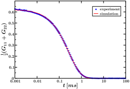
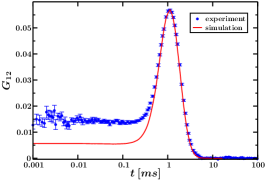
(c)	(d)
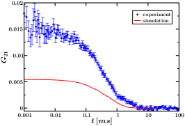
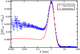
(e)	(f)
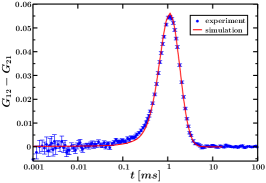
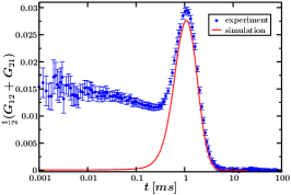
(g)	(h)

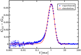
Figure 3: (Color online) Correlation functions $G_{ij}$ as defined in the text, and linear combinations thereof, comparing the experimental data (with error bars) with the numerical fit functions (without) for an optimized parameter set. The statistical error of the numerical data is smaller than the line width. Parts (a) – (f) have been obtained by modeling the observation volumes by Eq. 9, while for parts (g) and (h) we have assumed a Gaussian form (Eq. 6).

Figure 3 summarizes our experimental results for the $G_{ij}$ and / or linear combinations thereof. Concerning the autocorrelation curves $G_{11}$ and $G_{22}$, we find that they are practically identical, which means that for the modeling it is safe to assume that both pinholes have the same properties. This is clearly shown in part (a), where one sees that $G_{11}-G_{22}$ differs only marginally from zero (while in our model we have anyway strictly $G_{11}=G_{22}$). Therefore, we just used the arithmetic mean $(G_{11}+G_{22})/2$ (part (b)) as autocorrelation input for our fits, while we discarded the $G_{11}-G_{22}$ data. Concerning the cross-correlations, one sees that the forward function $G_{12}$ (see part (c)) exhibits a pronounced peak, which is indicative of the typical time that a particle needs to travel from observation volume 1 to observation volume 2. Another striking feature of $G_{12}$ is the large plateau for small times. At such short times, the particles have essentially not moved at all. Hence the plateau indicates that a particle is able to send photons to both detectors from essentially the same position, or, in other words, that the effective observation volumes must overlap quite substantially. This overlap effect then of course also shows up in the backward correlation function $G_{21}$ (see part (d)) at short times, with precisely the same plateau value. Therefore, such overlap effects essentially cancel out when considering the difference $G_{12}-G_{21}$ instead (see part (f)), while of course they are strongly present in the mean $(G_{12}+G_{21})/2$ (see part (e)).

Obviously, the source of the overlap must be an effect of the optical imaging system, which is of course somewhat complicated, due to the many components that are involved. However, beyond this general statement we have unfortunately so far been unable to trace down its precise physical origin, and therefore also been unable to construct a fully consistent model for the observation volumes. The simple models that we have considered in our present work are not fully adequate, meaning that they systematically underestimate the amount of overlap, unless one assumes highly unphysical parameters, which would cause other aspects of the modeling to fail completely. It should be noted that similar overlap effects are also present in standard double-beam FCCS Rigler01 ; however, the underlying physics for that setup is slightly different, and the modeling used there cannot be simply transferred to our system.

Fortunately, however, our best model for the observation volumes is at least physical enough such that it can describe not only the autocorrelation functions (see part (b)) but also the overlap-corrected difference $G_{12}-G_{21}$ (part (f)) reasonably well, while still failing to describe the mean $(G_{12}+G_{21})/2$ (part (e)). For this reason, our fitting procedure altogether takes into account the linear combinations $(G_{11}+G_{22})/2$ and $G_{12}-G_{21}$, while deliberately discarding the data on $(G_{12}+G_{21})/2$ and $G_{11}-G_{22}$. This is nicely borne out in Fig. 3, which shows not only the experimental data, but also the result of our theoretical modeling for optimized parameters.

The fact that the success of the modeling depends crucially on an accurate description of the observation volumes is strongly underpinned by parts (g) and (h) of Fig. 3. The experimental data for $(G_{12}+G_{21})/2$ and $G_{12}-G_{21}$ are again the same, but the theoretical model uses a different functional form for the observation volumes, whose performance is obviously significantly poorer: Not only is the overlap plateau (part (g)) underestimated even more strongly than for the better model (part (e)), but also in the overlap-corrected function $G_{12}-G_{21}$ (part (h)) are the deviations from the experimental data much more pronounced than for the better model (part (f)). It should also be noted that the autocorrelation functions are much less sensitive to these details; the autocorrelation curve for the poorer model (data not shown) fits the experiments as well as the better one (part (b)).

IV Correlation Functions and Particle Dynamics

IV.1 Molecular Detection Efficiency

The fluorescence particles pass consecutively through the two observation volumes $W_{1}$ and $W_{2}$ (Fig. 2). The observation volume of each pinhole is given by the space-dependent molecular detection efficiency (MDE) function. It depends on the excitation intensity profile $I_{z}(z)$, and the collection efficiency of the objective plus detector system. In essence, the function $W_{1}(\boldsymbol{r})$ denotes the probability density for the event that a fluorescence photon emitted from a particle at position $\boldsymbol{r}$ will pass through pinhole $1$ and reach detector $1$. Similarly, $W_{2}(\boldsymbol{r})$ is the analogous function for pinhole $2$. Since the intensity of the evanescent wave decays exponentially with a penetration depth $d_{p}$ (of order $100nm$), and the observation volumes are displaced with respect to one another by a distance $s_{x}$ (roughly $800nm$), we assume the functional form

$$W_{1}(\boldsymbol{r}) = W_{xy}\left(x,y\right)d_{p}^{-1}\exp\left(-\frac{z}{d_{p}}\right),$$ (3)

$$W_{2}(\boldsymbol{r}) = W_{xy}\left(x-s_{x},y\right)d_{p}^{-1}\exp\left(-\frac{z}{d_{p}}\right),$$ (4)

where normalization of the probability densities implies

$$\int_{-\infty}^{\infty}dx\int_{-\infty}^{\infty}dyW_{xy}\left(x,y\right)=1.$$ (5)

In general the function $W_{xy}$ is given by the convolution of the pinhole image in the sample space with the point spread function (PSF) of the objective. However, one simple and widely used approximation, valid for pinholes equal or smaller than the Airy Unit of the system, assumes that $W_{xy}$ is a Gaussian function Rigler01 ; HasslerSecond05 ; zhangzerubia :

$$W_{xy}(x,y)=\frac{2}{\pi w_{0}^{2}}\exp\left(-2\frac{x^{2}+y^{2}}{w_{0}^{2}}\right);$$ (6)

a typical value for the width that we obtain from fitting is $w_{0}\simeq 250nm$.

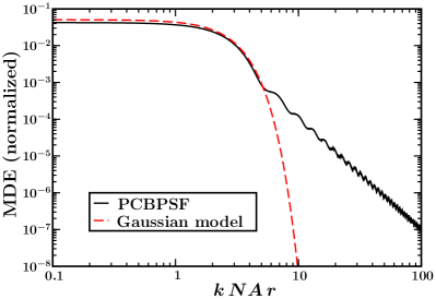
Figure 4: (Color online) Comparison of the two normalized MDEs used in our study, for the optimized parameters of Fig. 3, using the natural unit system of the PCBPSF.

A substantially better description of $W_{xy}$ can be obtained by considering the explicit form of the PSF webb ; richardswolf . However, this form is described with complex mathematical equations and is often approximated by a squared Bessel function webb ; bornwolf ; zhangzerubia

$$PSF_{xy}\propto\left(\frac{2J_{1}(q)}{q}\right)^{2},$$ (7)

where $J_{1}$ denotes the first Bessel function and

$$q=k\,NA\,\sqrt{x^{2}+y^{2}}=\frac{2\pi}{\lambda}\,NA\,\sqrt{x^{2}+y^{2}}.$$ (8)

Here $\lambda$ is the wavelength of the fluorescent light (in our case $600nm$). The Bessel PSF implicitly assumes a paraxial approximation (i. e. small $NA$). While this assumption is probably not the best for confocal microscopy, it is certainly more accurate than a simple Gaussian PSF webb ; zhangzerubia .

As mentioned above, in order to describe what a pinhole sees one must calculate the convolution of the PSF of the objective with the pinhole image in the sample space. The geometrical image of the pinhole is simply obtained by dividing the physical size of the pinhole (physical radius $=50\mu m$) by the total magnification of the system (in our case $\approx 333$). This results in a radius $R_{PH}$ in the sample space of approximately $150nm$. Therefore the total model MDE is given by zhangzerubia

$$W_{xy}(x,y)=\left(\frac{k\,NA}{2\pi R_{PH}}\right)^{2}\int_{\left|\boldsymbol{r_{0}}\right|\leq R_{PH}}d^{2}r_{0}\left(\frac{2J_{1}(q)}{q}\right)^{2},$$ (9)

where

$$q=k\,NA\,\sqrt{(x-x_{0})^{2}+(y-y_{0})^{2}}.$$ (10)

The convolution integral is difficult to evaluate analytically, but easy to calculate numerically. To this end, we use dimensionless length units in which the factor $kNA$ is unity. In these dimensionless units, $R_{PH}$ takes the value $2.3$ for the parameters given above, which is the value we have used throughout our study. We call this function (9) the “pinhole-convoluted Bessel point spread function” (PCBPSF), which we calculated in dimensionless units once and for all, and stored as a table. During the actual data analysis, the transformation factor from dimensionless units to real units was used as a fit parameter, in analogy to $w_{0}$ for the Gaussian model. It should be noted that the PCBPSF decays for large distances like $(x^{2}+y^{2})^{-3/2}$, therefore providing much more overlap than the Gaussian model.

In the present work, we have studied both models, the “Gaussian” model according to Eq. 6, as well as the PCBPSF model according to Eq. 9. The corresponding correlation curves have already been presented in Fig. 3. The corresponding MDEs are shown in Fig. 4. One sees that the PCBPSF model puts much more statistical weight into the tail of the distribution than the Gaussian model. As already discussed above, we found the Gaussian model to perform less well than the PCBPSF model, since it underestimates the overlap even more severely than the latter. In what follows, we will present data always for the PCBPSF model, unless stated differently.

IV.2 Theory of Correlation Functions

The dynamics of the tracer particles is described by the space- and time-dependent concentration (number of particles per unit volume) $C(\boldsymbol{r},t)$, its fluctuation

$$\delta C(\boldsymbol{r},t)=C(\boldsymbol{r},t)-\langle C\rangle$$ (11)

and the concentration correlation function

$$\Phi({\boldsymbol{r}},{\boldsymbol{r}}^{\prime},t)=\langle\delta C({\boldsymbol{r}},t)\delta C({\boldsymbol{r}}^{\prime},0)\rangle;$$ (12)

note that translational invariance applies only to time, but not to space, due to the presence of the flow and the surface. At time $t=0$, this reduces to the static correlation function, for which we simply assume the function pertaining to an ideal gas:

$$\Phi({\boldsymbol{r}},{\boldsymbol{r}}^{\prime},0)=\langle C\rangle\delta({\boldsymbol{r}}-{\boldsymbol{r}}^{\prime}).$$ (13)

Note that this assumption implies that we consider the particles as point particles, with no interaction with the surface except impenetrability, and no interaction between each other, due to dilution.

As described in Ref. Rigler01 , the correlation functions are related to $\Phi$ via

$$G_{ij}(t) = \frac{\int\int d^{3}rd^{3}r^{\prime}W_{i}({\boldsymbol{r}^{\prime}})W_{j}({\boldsymbol{r}})\Phi({\boldsymbol{r}},{\boldsymbol{r}^{\prime}},t)}{\langle C\rangle^{2}\left(\int d^{3}rW_{i}({\boldsymbol{r}})\right)\left(\int d^{3}rW_{j}({\boldsymbol{r}})\right)}$$

$$= \langle C\rangle^{-2}\int\int d^{3}rd^{3}r^{\prime}W_{i}({\boldsymbol{r}^{\prime}})W_{j}({\boldsymbol{r}})\Phi({\boldsymbol{r}},{\boldsymbol{r}^{\prime}},t),$$

where in the second step we have taken into account the normalization of the $W_{i}$. Therefore, the obvious strategy for analyzing the experimental data is to (i) evaluate $\Phi$ within a model for the particle dynamics, (ii) evaluate the integrals in Eq. IV.2 to obtain a theoretical prediction for $G_{ij}$ for a given set of parameters, (iii) compare the prediction with the data, and (iv) optimize the parameters. The normalizing prefactor $\langle C\rangle^{-2}$ is not known very accurately and will hence be treated as a fit parameter.

The tracer particles undergo a diffusion process and move in an externally driven flow field $\boldsymbol{v}$. Hence, we describe the concentration correlation function by a convection-diffusion equation of the form

$$\partial_{t}\Phi({\boldsymbol{r}},{\boldsymbol{r}}^{\prime},t)=D\nabla_{\boldsymbol{r}}^{2}\Phi({\boldsymbol{r}},{\boldsymbol{r}}^{\prime},t)-\nabla_{\boldsymbol{r}}\cdot{\boldsymbol{v}(\boldsymbol{r})}\Phi({\boldsymbol{r}},{\boldsymbol{r}}^{\prime},t),$$ (15)

which needs to be solved for $z\geq 0,z^{\prime}\geq 0$ with the initial condition Eq. 13 and the no-flux boundary condition at the surface,

$$\left.\partial_{z}\Phi({\boldsymbol{r}},{\boldsymbol{r}}^{\prime},t)\right|_{z=0}=0,$$ (16)

which imposes that there is no diffusive current entering the solid. For reasons of simplicity, the hydrodynamic interactions with the surface are neglected, and hence the diffusive term is described only by an isotropic diffusion constant $D$.

Since in the experiment the exponential decay length of the spatial detection volume normal to the surface is in the range of $100-200nm$, while the channel size is three orders of magnitude larger, it is justified to assume the flow field to be approximately linear. For our geometry, this implies

$$\boldsymbol{v}(\boldsymbol{r})=\dot{\gamma}\tensor{\boldsymbol{\varepsilon}}\cdot(\boldsymbol{r}+l_{s}\hat{\boldsymbol{e}}_{z}),$$ (17)

where $l_{s}$ is the slip length, $\dot{\gamma}=\partial v_{x}/\partial z$ is the constant shear rate, $\hat{\boldsymbol{e}}_{z}$ denotes the unit vector in $z$-direction and $\tensor{\boldsymbol{\varepsilon}}=\hat{\boldsymbol{e}}_{x}\otimes\hat{\boldsymbol{e}}_{z}$ is the dimensionless rate-of-strain tensor.

At this point, it is useful to re-define the coordinate system in such a way that the finite hard-sphere radius $R$ of the tracer particles (roughly $7nm$) is taken into account. We therefore identify $z=0$ no longer with the interface, but rather with the $z$ coordinate of the particle center at contact with the interface. In this new coordinate system, the flow field is given by

$$\boldsymbol{v}(\boldsymbol{r})=\dot{\gamma}\tensor{\boldsymbol{\varepsilon}}\cdot(\boldsymbol{r}+(l_{s}+R)\hat{\boldsymbol{e}}_{z}),$$ (18)

i. e. we simply have to add the particle radius to the slip length. The functional form of the observation volumes $W_{1}$ and $W_{2}$ remains unchanged, since the $z$ dependence is just an exponential decay, such that a shift in $z$ direction just results in a constant prefactor that can be absorbed in the overall normalization. Our method therefore does not yield a value for $l_{s}$, but rather only for the combination $l_{s}+R$.

As mentioned previously, for some special cases the convection-diffusion equation can be solved analytically, for example in the case of uniform or linear flow in bulk, i. e. far away from surfaces Lum03 ; Bri99 ; Elr62 ; Foi80 , or for pure diffusion close to the wall, but without any flow field Rie08 ; Hassler05 . For our case, however, it is not easy, or even impossible, to find such a solution. Therefore the aim of the next sections will be to construct a stochastic numerical method. Concerning the problems that were mentioned after Eq. IV.2, (i) and (ii) can be solved by Brownian Dynamics, while problems (iii) and (iv) are tackled by a Monte Carlo algorithm in parameter space.

V Sampling algorithm

Brownian motion of particles under the influence of external driving is described by a Fokker-Planck equation Ris96 ; Hon94 ; Oet96 ; Maz02 ; Lad03 , which has exactly the same form as the convection-diffusion equation, Eq. 15, the only difference being that $\Phi$ is replaced by the so-called “propagator” $P(\boldsymbol{r},t|{\boldsymbol{r}}^{\prime},0)$, which is the conditional probability density for the particle motion $\boldsymbol{r}^{\prime}\to\boldsymbol{r}$ within the time $t$. $P$ and $\Phi$ describe the same physics and are actually identical except for a trivial normalization factor, $\Phi=\langle C\rangle P$. We can therefore rewrite Eq. IV.2 as

$$\langle C\rangle G_{ij}(t)$$

$$= \int\int d^{3}rd^{3}r^{\prime}W_{i}({\boldsymbol{r}^{\prime}})W_{j}({\boldsymbol{r}})P(\boldsymbol{r},t|{\boldsymbol{r}}^{\prime},0).$$

As is well-known, the Fokker-Planck equation is equivalent to describing the particle dynamics in terms of a Langevin equation

$$\dot{\boldsymbol{r}}(t)={\boldsymbol{v}}({\boldsymbol{r}}(t))+{\boldsymbol{\eta}}(t).$$ (20)

Here $\dot{\boldsymbol{r}}(t)$ is the tracer velocity, ${\boldsymbol{v}}$ is the deterministic (external) velocity imposed by the flow, while ${\boldsymbol{\eta}}$ is a stochastic Gaussian white noise term which describes the diffusion:

$$\langle\eta_{\alpha}(t)\rangle = 0,$$ (21a)

$$\langle\eta_{\alpha}(t^{\prime})\eta_{\beta}(t)\rangle = 2D\delta_{\alpha\beta}\delta(t^{\prime}-t).$$ (21b)

Here, $\alpha,\beta=x,y,z$ are Cartesian indices and $\delta_{\alpha\beta}$ is the Kronecker delta. We solve this Langevin equation numerically by means of a simple Euler algorithm Oet96 with a finite time step $\Delta t$:

$$\boldsymbol{r}(t+\Delta t)=\boldsymbol{r}(t)+\Delta t{\boldsymbol{v}}({\boldsymbol{r}}(t))+\sqrt{2D\Delta t}{\boldsymbol{\chi}},$$ (22)

where $\boldsymbol{\chi}=(\chi_{x},\chi_{y},\chi_{z})$ is a vector of mutually independent random numbers with mean $0$ and variance $1$. The boundary condition at the wall is taken into account by a simple reflection at $z=0$, i. e. a particle that, after a certain time step, has entered the negative half-space $z<0$ is subjected to $z\to-z$ before the next propagation step is executed.

Now, let us consider a computer experiment where, at time $t=0$, we place a particle randomly in space, with probability density $\rho_{0}(\boldsymbol{r^{\prime}})$, and then propagate it stochastically according to Eq. 22. The probability density for it reaching the position $\boldsymbol{r}$ after the time $t$ is then given by

$$Q(\boldsymbol{r},t)=\int d^{3}r^{\prime}P(\boldsymbol{r},t|{\boldsymbol{r}}^{\prime},0)\rho_{0}(\boldsymbol{r^{\prime}}).$$ (23)

If we now consider an observable $A$, which is some function of the particle’s coordinate, $A=A(\boldsymbol{r})$, and study the time evolution of its average, then this is obviously given by

$$\langle A\rangle(t) = \langle A(\boldsymbol{r}(t))\rangle$$

$$= \int d^{3}rA(\boldsymbol{r})Q(\boldsymbol{r},t)$$

$$= \int\int d^{3}rd^{3}r^{\prime}A(\boldsymbol{r})P(\boldsymbol{r},t|{\boldsymbol{r}}^{\prime},0)\rho_{0}(\boldsymbol{r^{\prime}}).$$

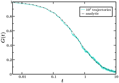
Figure 5: (Color online) Analytical solution and simulated data for an average over $10^{3}$ trajectories.

Therefore, if we set $\rho_{0}=W_{i}$ and $A=W_{j}$, then $\left<A\right>$ is identical to the rescaled correlation function $\langle C\rangle G_{ij}$. In other words, we place the particle initially with probability density $W_{i}$, then generate a stochastic trajectory via Eq. 22, and evaluate $W_{j}$ for all times along that trajectory. This yields a function $W_{j}(t)$ for that particular trajectory. This computer experiment is repeated often, and averaging $W_{j}(t)$ over all trajectories yields directly a stochastic estimate for the (unnormalized) correlation function $G_{ij}$. Of course, these estimates will have statistical error bars, just as the experimental ones; however, we sample several hundred thousand trajectories, such that the numerical errors are substantially smaller than the experimental ones. In principle, the numerical data are also subject to a systematic discretization error as a result of the finite time step; however, by choosing a small value for $\Delta t$ we have made sure that this is still small compared to the statistical uncertainty. Note also that our approach implements an optimal importance sampling Lan00 with respect to the $t=0$ factor $W_{i}$, but not with respect to $W_{j}$. In practical terms, our straightforward sampling scheme turned out to be absolutely adequate.

The simulations were run using a “natural” unit system where length units are defined by setting $d_{p}$ to unity, while the time units are given by setting the diffusion constant $D$ to unity. The time step was fixed in physical units to a value of at most $2\mu s$ (it was dynamically adjusted in order to match the non-equidistant experimental observation times), which, for all parameters, is much smaller than unity in dimensionless units. Obviously, this is small enough to represent the stochastic part of the Langevin update scheme with sufficient accuracy. For typical parameters ($D=35\mu m^{2}/s$, $d_{p}=0.1\mu m$, $\dot{\gamma}=4\times 10^{3}s^{-1}$), the dimensionless unit time corresponds to $\simeq 0.3ms$, such that the resulting value for the dimensionless shear rate ($\simeq 1.2$) is of order unity as well. Since $d_{p}$ (or unity, in dimensionless units) defines the $z$ range in which the statistically relevant part of the simulation takes place, we find that typical flow velocities in dimensionless units are also of order unity. This shows that the time step is also small enough for the deterministic part of the Langevin equation. We also see that the experiment is neither dominated by diffusion nor by convection, and therefore the analysis needs to take into account both.

As a simple test case, we used our algorithm to calculate the autocorrelation function for vanishing flow and the Gaussian model for the observation volume, where an analytical solution is known Hassler05 ; Rie08 . In our dimensionless units, it is, up to a constant prefactor, given by

$$G^{(\mathrm{a})}(t)$$

$$= \left(1+\frac{4t}{w_{0}^{2}}\right)^{-1}\left(\left(1-2t\right)\exp\left(t\right)\mathrm{erfc}\left[\sqrt{t}\right]+\sqrt{\frac{4}{\pi}t}\right).$$

Figure 5 shows the analytic autocorrelation function with $w_{0}=2$ and its simulated counterpart, averaged over $10^{3}$ independent trajectories, where a small time step of $\Delta t=10^{-3}$ (in dimensionless units) was used. In Fig. 6 the deviation of the simulated data ($G^{(\mathrm{s})}$) from the analytic expression is shown,

$$\mathrm{error}(t)=G^{(\mathrm{s})}(t)-G^{(\mathrm{a})}(t).$$ (26)

Clearly, the numerical solution converges to the analytical result when the number of trajectories is increased, as it should be.

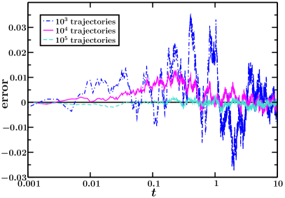
Figure 6: (Color online) Deviation from the analytic curve for $10^{3}$,$10^{4}$ and $10^{5}$ trajectories.

VI Subtraction Scheme

At this point, it is worthwhile to reconsider the subtraction procedure introduced in Sec. III. To this end, we assume that the true functions $W_{i}$ differ somewhat from the model functions, which we will denote by $W_{i}^{(m)}$. This is most easily parameterized by the ansatz

$$W_{i}=\left(1-\varepsilon\right)W_{i}^{(m)}+\varepsilon\tilde{W}_{i},$$ (27)

where $W_{i}$, $W_{i}^{(m)}$ and $\tilde{W}_{i}$ are all normalized to unity, while $\varepsilon$ is a (hopefully) small parameter. For the purposes of the present analysis, we also assume that the Brownian Dynamics model is a faithful and correct description of the true dynamics, i. e. that the difference between $W_{i}$ and $W_{i}^{(m)}$ is the only reason for a systematic deviation between simulation and experiment.

Inserting Eq. 27 into Eq. V, we thus find

$$\langle C\rangle G_{ij}(t)$$

$$= \left(1-\varepsilon\right)^{2}\int\int d^{3}rd^{3}r^{\prime}W_{i}^{(m)}({\boldsymbol{r}^{\prime}})W_{j}^{(m)}({\boldsymbol{r}})P(\boldsymbol{r},t|{\boldsymbol{r}}^{\prime},0)$$

$$+ \varepsilon\left(1-\varepsilon\right)\int\int d^{3}rd^{3}r^{\prime}W_{i}^{(m)}({\boldsymbol{r}^{\prime}})\tilde{W}_{j}({\boldsymbol{r}})P(\boldsymbol{r},t|{\boldsymbol{r}}^{\prime},0)$$

$$+ \varepsilon\left(1-\varepsilon\right)\int\int d^{3}rd^{3}r^{\prime}\tilde{W}_{i}({\boldsymbol{r}^{\prime}})W_{j}^{(m)}({\boldsymbol{r}})P(\boldsymbol{r},t|{\boldsymbol{r}}^{\prime},0)$$

$$+ \varepsilon^{2}\int\int d^{3}rd^{3}r^{\prime}\tilde{W}_{i}({\boldsymbol{r}^{\prime}})\tilde{W}_{j}({\boldsymbol{r}})P(\boldsymbol{r},t|{\boldsymbol{r}}^{\prime},0).$$

Since we treat $\langle C\rangle$ as an adjustable parameter, it makes sense to view the first term (including the prefactor $\left(1-\varepsilon\right)^{2}$) as the theoretical model for the correlation function, $\left<C\right>G_{ij}^{(m)}(t)$. For the deviation between experiment and theory we then obtain, neglecting all terms of order $\varepsilon^{2}$,

$$K_{ij} := \varepsilon^{-1}\langle C\rangle\left(G_{ij}-G_{ij}^{(m)}\right)$$

$$= \int\int d^{3}rd^{3}r^{\prime}W_{i}^{(m)}({\boldsymbol{r}^{\prime}})\tilde{W}_{j}({\boldsymbol{r}})P(\boldsymbol{r},t|{\boldsymbol{r}}^{\prime},0)$$

$$+ \int\int d^{3}rd^{3}r^{\prime}\tilde{W}_{i}({\boldsymbol{r}^{\prime}})W_{j}^{(m)}({\boldsymbol{r}})P(\boldsymbol{r},t|{\boldsymbol{r}}^{\prime},0),$$

and for its antisymmetric part

$$K_{ij}-K_{ji}$$

$$= \int\int d^{3}rd^{3}r^{\prime}[W_{i}^{(m)}({\boldsymbol{r}^{\prime}})\tilde{W}_{j}({\boldsymbol{r}})$$

$$-W_{i}^{(m)}({\boldsymbol{r}})\tilde{W}_{j}({\boldsymbol{r}^{\prime}})]P(\boldsymbol{r},t|{\boldsymbol{r}}^{\prime},0)$$

$$- \int\int d^{3}rd^{3}r^{\prime}[W_{j}^{(m)}({\boldsymbol{r}^{\prime}})\tilde{W}_{i}({\boldsymbol{r}})$$

$$-W_{j}^{(m)}({\boldsymbol{r}})\tilde{W}_{i}({\boldsymbol{r}^{\prime}})]P(\boldsymbol{r},t|{\boldsymbol{r}}^{\prime},0).$$

The terms in square brackets are antisymmetric under the exchange $\boldsymbol{r}\leftrightarrow\boldsymbol{r}^{\prime}$, and hence $P$ can be replaced by its antisymmetric part

$$P_{a}(\boldsymbol{r},{\boldsymbol{r}}^{\prime},t)=P(\boldsymbol{r},t|{\boldsymbol{r}}^{\prime},0)-P(\boldsymbol{r}^{\prime},t|{\boldsymbol{r}},0).$$ (31)

Exchanging the arguments in the second terms within the square brackets then yields

$$\frac{1}{2}\left(K_{ij}-K_{ji}\right)$$

$$= \int\int d^{3}rd^{3}r^{\prime}W_{i}^{(m)}({\boldsymbol{r}^{\prime}})\tilde{W}_{j}({\boldsymbol{r}})P_{a}(\boldsymbol{r},{\boldsymbol{r}}^{\prime},t)$$

$$- \int\int d^{3}rd^{3}r^{\prime}W_{j}^{(m)}({\boldsymbol{r}^{\prime}})\tilde{W}_{i}({\boldsymbol{r}})P_{a}(\boldsymbol{r},{\boldsymbol{r}}^{\prime},t).$$

This is clearly a nonzero contribution. In other words, the subtraction scheme (i. e. studying $G_{12}-G_{21}$ instead of $G_{12}$) does not provide a consistent cancellation procedure such that the first-order deviation would vanish. However, in practical terms the deviation is much smaller than for the original data ($G_{12}$ and $G_{21}$), for which Eq. VI applies. To some extent, this is so because the error is the difference of two terms, but mostly it is due to the fact that not the full propagator $P$ contributes, but rather only its antisymmetric part $P_{a}$. For short times the dynamics is dominated by diffusion, i. e. $P$ is essentially symmetric, or $P_{a}\approx 0$. At late times, we again expect $P_{a}$ to become quite small (exponentially damped, see Eq. VI), although we have no rigorous proof for this. Therefore one should expect that the strongest deviation occurs at intermediate times where $P_{a}$ is maximum. This time scale is not given by the optical geometry but rather by the dynamics; dimensional analysis then tells us that this time must be of order $D/v^{2}$. For typical parameters of our experiment ($D=35\mu m^{2}/s$, $v=4\times 10^{2}\mu m/s$) we obtain a value of roughly $0.2ms$, which fits quite well to the observations one can make in Fig. 3, part (h). At such times, we expect that the main contribution to $K_{12}-K_{21}$ comes form the first term of Eq. VI (downstream vs. upstream correlation) and that $P_{a}$ is positive for most of the relevant arguments. Therefore, one should expect that the experimental data should lie systematically above the theoretical predictions, which is indeed the case. Our expectations concerning the behavior of $P_{a}$ come from studying the simple case of one-dimensional diffusion with constant drift without boundary conditions; here one has

$$P(x,t|x^{\prime},0)=\frac{1}{\sqrt{4\pi Dt}}\exp\left(-\frac{(x-x^{\prime}-vt)^{2}}{4Dt}\right)$$ (33)

and

$$P_{a}(x,x^{\prime},t) = \frac{2}{\sqrt{4\pi Dt}}\exp\left(-\frac{(x-x^{\prime})^{2}}{4Dt}\right)$$

$$\exp\left(-\frac{v^{2}t}{4D}\right)\sinh\left(\frac{(x-x^{\prime})v}{2D}\right).$$

VII Statistical Data Analysis

VII.1 Monte Carlo Algorithm

For the model that we consider in the present paper, the space of fit parameters is (in principle) seven-dimensional. We have three lengths that define the geometry of the optical setup, $d_{p}$, $s_{x}$, and $w_{0}$ (Gaussian model) or $(k\,NA)^{-1}$ (diffraction model). Three further parameters define the properties of the flow and the diffusive dynamics of the tracers; these are the diffusion constant $D$, the shear rate $\dot{\gamma}$, and the slip length plus particle radius $l_{s}+R$. Finally, there is the concentration of tracer particles $\langle C\rangle$, which serves as a global normalization constant. The functions to be fitted are $(G_{11}+G_{22})/2$ and $G_{12}-G_{21}$. However, we have seen in Sec. VI that the non-idealities in modeling the observation volumes do have an effect on the normalizations, and therefore we allowed one separate normalization constant $\langle C\rangle$ for each of the curves ($\langle C\rangle_{A}$ for the autocorrelation and $\langle C\rangle_{C}$ for the cross-correlation), in order to partly compensate for these non-idealities. Therefore, our parameter space is finally eight-dimensional. The strategy that we develop in the present section aims at adjusting all parameters simultaneously in order to obtain optimum fits. For the further development, it will be useful to combine all the parameters into one vector $\boldsymbol{\Pi}$. Furthermore, for each parameter we can, from various physical considerations, define an interval within which it is allowed to vary (because values outside that interval would be highly unreasonable or outright unphysical). This means that we restrict the consideration to a finite eight-dimensional box $\Omega_{\boldsymbol{\Pi}}$ in parameter space.

A central ingredient of our approach is the fact that both the experimental data and the simulation results have been obtained with good statistical accuracy ($\simeq 2.5\times 10^{5}$ trajectories for the simulations, $40$ independent measurements for the experiments). This does not only allow us to obtain rather small statistical error bars, but also (even more importantly) to rely on the asymptotics of the Central Limit Theorem, i. e. to assume Gaussian statistics throughout. For both correlation curves and each of the considered times, we have both an experimental data point $E_{i}$ and a simulated data point $S_{i}$, where the index $i$ simply enumerates the data points. Both $E_{i}$ and $S_{i}$ can be considered as Gaussian random variables with variances $\sigma_{E,i}^{2}$ and $\sigma_{S,i}^{2}$, respectively. Then

$$\tilde{\Delta}_{i}=\frac{S_{i}-E_{i}}{\sqrt{\sigma_{S,i}^{2}+\sigma_{E,i}^{2}}}$$ (35)

is again a Gaussian random variable, whose variance is simply unity,

$$\left<\tilde{\Delta}_{i}^{2}\right>-\left<\tilde{\Delta}_{i}\right>^{2}=1.$$ (36)

Therefore, $\tilde{\Delta}_{i}$ is, in principle, a perfect variable to measure the deviation between simulation and experiment. Unfortunately, however, the parameters $\sigma_{S,i}$ and $\sigma_{E,i}$ are not known. What is rather known are their estimators $s_{S,i}$ and $s_{E,i}$, as they are obtained from standard analysis to calculate error bars. Therefore, we rather consider

$$\Delta_{i}=\frac{S_{i}-E_{i}}{\sqrt{s_{S,i}^{2}+s_{E,i}^{2}}}.$$ (37)

The statistical properties of this variable, however, are in the general case unknown Wel38 . It is only in the case of rather good statistics (as we have realized it) that we can ignore the difference between $\sigma$ and $s$, and simply assume that $\Delta_{i}$ is indeed a Gaussian variable with unit variance. It is at this point where the statistical quality of the data clearly becomes important.

If $M$ is the total number of data points, then

$${\cal H}=\frac{1}{2}\sum_{i=1}^{M}\Delta_{i}^{2}$$ (38)

is obviously a quantity that measures rather well the deviation between experiment and simulation. In principle, the task is to pick the parameter vector $\boldsymbol{\Pi}$ in such a way that ${\cal H}$ is minimized. We have deliberately chosen the symbol ${\cal H}$ in order to point out the analogy to the problem of finding the ground state of a statistical-mechanical Hamiltonian. In case of a perfect fit, we have $\left<S_{i}\right>=\left<E_{i}\right>$ or $\left<\Delta_{i}\right>=0$, implying $\left<{\cal H}\right>=M/2$. In the standard nomenclature of fitting problems, $2{\cal H}$ is called “chi squared”. We also introduce $\xi=2{\cal H}/M$, which we will call the “goodness of simulation” (standard nomenclature: “chi squared per degree of freedom”).

For optimizing $\boldsymbol{\Pi}$, we obviously need to consider ${\cal H}$ as a function of $\boldsymbol{\Pi}$. In this context, it turns out that it is important to be able to consider it as a function of only $\boldsymbol{\Pi}$, and to make sure that this dependence is smooth. For this reason, we use the same number of trajectories when going from one parameter set to another one, and use exactly the same set of random numbers to generate the trajectories. In other words, the trajectories differ only due to the fact that the parameters were changed. Therefore, both $S_{i}$ and $s_{S,i}$ are smooth functions of the parameters, and ${\cal H}$ is as well.

In order to find the optimum parameter set, one could, in principle, construct a regular grid in $\Omega_{\boldsymbol{\Pi}}$ and then evaluate ${\cal H}$ for every grid point. However, for high-dimensional spaces (and eight should in this context be viewed as already a fairly large number, in particular when taking into account that it is bound to increase further as soon as more refined models are studied), it is usually more efficient to scan the space by an importance-sampling Monte Carlo procedure based upon a Markov chain Lan00 . Applying the standard Metropolis scheme Lan00 , we thus arrive at the following algorithm:

1. Choose some start vector $\boldsymbol{\Pi}$. This should be a reasonable set of parameters, perhaps pre-optimized by simple visual fitting.

2. From the previous set of parameters, generate a trial set via $\boldsymbol{\Pi}^{\prime}=\boldsymbol{\Pi}+\Delta\boldsymbol{\Pi}$, where $\Delta\boldsymbol{\Pi}$ is a random vector chosen from a uniform distribution from a small sub-box aligned with $\Omega_{\boldsymbol{\Pi}}$.

3. If the new vector is not within $\Omega_{\boldsymbol{\Pi}}$, reject the trial set and go to step 2.

4. Otherwise, calculate both $P_{eq}(\boldsymbol{\Pi}^{\prime})$ and $P_{eq}(\boldsymbol{\Pi})$, as well as the Metropolis function

   $$m=\min\left(1,P_{eq}(\boldsymbol{\Pi}^{\prime})/P_{eq}(\boldsymbol{\Pi})\right),$$ (39)

   where $P_{eq}$ is the “equilibrium” probability density of $\boldsymbol{\Pi}$, i. e. the desired probability density towards which the Markov chain converges (more about this below).

5. Accept the trial move with probability $m$ (reject it with probability $1-m$), count either the accepted or the old set as a new set in the Markov chain, and go to step 2.

6. After relaxation into equilibrium, sample desired properties of the distribution of $\boldsymbol{\Pi}$, like mean values, variances, covariances, etc., by simple arithmetic means over the parameter sets that have been generated by the Markov chain. This allows the estimation of not only the physical parameters, but at the same time also of their statistical error bars.

The scheme is defined as soon as $P_{eq}$ is specified. Now, from the considerations above, we know that in case of a perfect fit the variables $\Delta_{i}$ are independent Gaussians with zero mean and unit variance. This implies (ignoring constant prefactors which anyway cancel out in the Metropolis function)

$$P_{eq} \propto \prod_{i}\exp\left(-\frac{1}{2}\Delta_{i}^{2}\right)$$ (40)

$$= \exp\left(-\frac{1}{2}\sum_{i}\Delta_{i}^{2}\right)$$

$$= \exp\left(-{\cal H}\right),\$$

which makes the interpretation in terms of statistical mechanics obvious. Clearly, this form for $P_{eq}$ is the only reasonable choice for implementing the Monte Carlo algorithm. After relaxation into equilibrium, one should observe a $\xi$ value of roughly unity, while larger numbers indicate a non-perfect fit (even after exhaustive Monte Carlo search), and thus deficiencies in the theoretical model. One should also be aware that the equilibrium fluctuations of $\xi$ are expected to be quite small, since $\xi$ is the arithmetic mean of a fairly large number ($M$, the number of experimental data points) of independent random variables.

In practice, we adjusted $\Delta\boldsymbol{\Pi}$ in order to obtain a fairly large acceptance rate of roughly $0.6\ldots 0.8$. The Monte Carlo algorithm was then run for more than $3\times 10^{5}$ steps, each step involving the generation of roughly $2.5\times 10^{5}$ trajectories. The simulation was run on $512$ nodes ($2048$ processes) of the IBM Blue Gene-P at Rechenzentrum Garching, where each process generated $123$ trajectories. On this machine, one Monte Carlo run took roughly one day to complete. It turned out that discarding the first $5\times 10^{4}$ configurations was sufficient to obtain data in equilibrium conditions, where the mean values of the parameters and their standard deviations were calculated. It should be noted that the equilibrium fluctuations of the parameters tell us the typical range in which they can still be viewed as compatible with the experiments. Therefore these fluctuations are the appropriate measure to quantify the experimental error bars, while calculating a standard error of mean (or a similar quantity) would not be appropriate and severely underestimate the errors. Finally, it should be noted that the approach allows in principle to analyze the mutual dependence of the parameters as well, by sampling the corresponding covariances; this was however not done in the present study.

VII.2 Scale Invariance

As noted before, the correlation functions depend on the average concentration $\langle C\rangle$, the diffusion constant $D$, the shear rate $\dot{\gamma}$, and various lengths, which we denote by $\{l_{i}\}$. Simple dimensional analysis shows that for any scale factor $a$ the scaling relation

$$G_{ij}(t,\langle C\rangle,D,\dot{\gamma},\{l_{i}\})$$

$$= G_{ij}\left(t,a^{3}\langle C\rangle,D/a^{2},\dot{\gamma},\left\{l_{i}/a\right\}\right)$$

holds. The “Hamiltonian” of the previous subsection is of course subject to the same scale invariance. This means that for each point in parameter space there is a whole “iso-line” in parameter space that fits the data just as well as the original point. Therefore, in order to improve the MC sampling, we generated such an iso-line for each point in parameter space that was produced by the Markov chain of the previous subsection. Of course, the iso-lines were confined to the region of the overall parameter box. It turned out that our Markov chains were still so short that this improvement was not completely superfluous (as it would be in the limit of very long chains). In other words, taking the invariance into account helped us to avoid underestimating the errors.

In practice, this was done as follows: Assuming that the most accurate input parameters are the penetration depth $d_{p}=100\pm 10nm$, the diffusion constant $D=36\pm 5\mu m^{2}/s$ and the separation distance $s_{x}=800\pm 80nm$, we calculate for every data point a minimum and a maximum scaling factor $a$, such that we obtain $d_{p}^{(min)}<a^{-1}d_{p}<d_{p}^{(max)}$, $s_{x}^{(min)}<a^{-1}s_{x}<s_{x}^{(max)}$ and $D^{(min)}<a^{-2}D<D^{(max)}$, for all $a$ in $(a_{min},a_{max})$. This provides us with additional data points in parameter space that are added to the statistics.

VII.3 Sample-to-Sample Fluctuations

seed	42		4711		2409
	av	$\sigma$	av	$\sigma$	av	$\sigma$
$\langle C\rangle_{A}[\mu m^{-3}]$	$17.83$	$1.92$	$17.81$	$1.96$	$17.94$	$1.94$
$\langle C\rangle_{C}[\mu m^{-3}]$	$16.53$	$1.80$	$16.45$	$1.82$	$16.83$	$1.83$
$d_{p}[nm]$	$95.81$	$3.50$	$96.02$	$3.58$	$95.78$	$3.52$
$(kNA)^{-1}[nm]$	$68.70$	$2.60$	$68.58$	$2.61$	$69.81$	$2.69$
$s_{x}[nm]$	$781.94$	$27.70$	$779.54$	$28.28$	$793.22$	$28.24$
$D[\mu m^{2}/s]$	$36.59$	$2.56$	$36.47$	$2.62$	$36.63$	$2.57$
$l_{s}+R[nm]$	$12.80$	$1.10$	$11.62$	$0.90$	$15.14$	$1.21$
$\xi$	$1.441$	$0.018$	$1.277$	$0.016$	$1.718$	$0.017$
acceptance rate	$82.0\%$		$82.0\%$		$82.2\%$
No. of MC steps	$609410$		$609590$		$610510$

Table 1: Averaged values (av) and standard deviations ($\sigma$) calculated from MC simulations with fixed $\dot{\gamma}=3800s^{-1}$, but different start values (“seeds”) for the random number generator.

It should be noted that the parameters found by the procedure outlined above are optimized for a specific set of random numbers used to generate the trajectories. Therefore, one must expect that one obtains different results when changing the set of random numbers. In our statistical-mechanical picture, we may view the set of random numbers as random “coupling constants” of a disordered system like a spin glass mezard , where the disorder is weak since the number of trajectories is large. For disordered systems, the phenomenon of “sample-to-sample” fluctuations is well-known, and it should be taken into account. We have therefore run one test where we applied the same analysis to three different random number sequences. Indeed we found (see Tab. 1) that sample-to-sample fluctuations are observable, and somewhat larger than the errors obtained from simple MC, while still being of the same order of magnitude. A conservative error estimate should therefore take these fluctuations into account, by multiplying the error estimates from plain MC by, say, a factor of three. In what follows, we will only report the simple MC estimates for the errors.

VIII Results

Figure 7: Goodness of simulation $\xi$ as function of the number of Monte Carlo steps for $\dot{\gamma}=3800s^{-1}$.

Figure 8: Slip length plus particle radius as function of the number of Monte Carlo steps for $\dot{\gamma}=3800s^{-1}$.

The experiments were performed with a penetration depth of the evanescent wave of $d_{p}\simeq 100nm$, the lateral size of the observation volumes (within the Gaussian model) was $w_{0}\simeq 250nm$ and their center-to-center separation was $s_{x}\simeq 800nm$. Furthermore, the diffusion constant of the tracers is known to be roughly $D\simeq 36\mu m^{2}/s$ as measured by dynamic light scattering. The shear rate was determined from an independent measurement using single-focus confocal FCS Dit02 ; Kohler2000 where the entire flow profile across the microchannel was mapped out. Alternatively, one might also use double-focus confocal FCCS Bri99 ; Lum03 . From this measurement, we obtained a shear rate at the bottom channel wall of $\dot{\gamma}=3854\pm 32s^{-1}$. More details on this issue and some theoretical background are presented in the appendix. Nevertheless, we took a conservative approach and allowed the shear rate to vary between $3500s^{-1}$ and $4000s^{-1}$. Finally, we expected the slip length to be not more than a few nanometers, but we nevertheless allowed it to vary up to $\simeq 100nm$. These estimates allowed us to start the Monte Carlo procedure with good input values.

We then observed the Monte Carlo simulation to systematically drift to smaller and smaller values of $\dot{\gamma}$, until finally “getting stuck” at the imposed lower boundary, $\dot{\gamma}=3500s^{-1}$. What we mean by this term is a behavior where fluctuations near $3500s^{-1}$ still occur, but in such a way that $3500s^{-1}$ is the most probable value, while smaller values only do not occur because we do not allow them. Since we know experimentally that $\dot{\gamma}=3500s^{-1}$ is clearly unacceptable, this behavior again indicates that the theoretical model is not completely sufficient to describe the experimental data (see also the discussion in Secs. III and VI).

We therefore decided to keep $\dot{\gamma}$ fixed during a Monte Carlo run, and rather vary it systematically in the given range. For none of the parameters were we able to obtain a better goodness of simulation than $\xi\simeq 1.25$, which is still a bit too large, i. e. indicates a non-perfect fit (although the data on $(G_{12}+G_{21})/2$ have been discarded already). The convergence behavior of the method is shown in Fig. 7, where we plot $\xi$ as a function of the number of Monte Carlo iterations. For the Gaussian model, the best $\xi$ value that we could obtain was $\xi\simeq 2.5$, which is substantially worse.

Figure 9: Averaged slip length as function of the shear rate, calculated from the Monte Carlo results.

With these caveats in mind, we may proceed to study the parameter values that the Monte Carlo procedure yields. Obviously, the most interesting one is the slip length $l_{s}$, or the sum $l_{s}+R$ (recall that the method does not provide an independent estimate for these parameters, but only for their sum). Figure 8 presents data on the evolution of $l_{s}+R$ during the Monte Carlo process for $\dot{\gamma}=3800s^{-1}$; $l_{s}+R$ is thus seen to fluctuate between roughly $10nm$ and $15nm$, which is, within the limitations of the model, the statistical experimental uncertainty of this quantity. The mean and standard deviation of $l_{s}+R$ is shown in Fig. 9 as a function of shear rate, which are thus clearly seen to not be independent. Since we know $\dot{\gamma}$ much more accurately than the range plotted in Fig. 9, we see that in principle a fairly accurate determination of $l_{s}$ is possible, if the underlying theoretical model is detailed enough to fully describe the physics. One should note that the particle size $R$ (more precisely, its hydrodynamic radius) is roughly $7nm$; taking this into accunt as well, we find a value that is clearly smaller than $10nm$. One should also note that for the Gaussian model we obtained a very similar curve; however, here the $l_{s}+R$ values are systematically smaller by roughly $5nm$. This again highlights the importance of having an accurate model for the MDE.

The other results obtained from our MC fits are reported in Tab. 2.

$\dot{\gamma}[s^{-1}]$	3500		3600		3700
	av	$\sigma$	av	$\sigma$	av	$\sigma$
$\langle C\rangle_{A}[\mu m^{-3}]$	$17.82$	$1.90$	$17.91$	$1.88$	$17.93$	$1.89$
$\langle C\rangle_{C}[\mu m^{-3}]$	$19.94$	$1.82$	$17.00$	$1.80$	$16.82$	$1.78$
$d_{p}[nm]$	$95.83$	$3.46$	$95.66$	$3.42$	$95.64$	$3.44$
$(kNA)^{-1}[nm]$	$68.84$	$2.53$	$69.10$	$2.55$	$69.01$	$2.56$
$s_{x}[nm]$	$774.39$	$26.59$	$777.98$	$26.63$	$780.53$	$26.97$
$D[\mu m^{2}/s]$	$36.71$	$2.49$	$36.76$	$2.48$	$36.72$	$2.51$
$l_{s}+R[nm]$	$21.92$	$1.31$	$19.16$	$1.24$	$15.98$	$1.12$
$\xi$	$1.377$	$0.016$	$1.40$	$0.016$	$1.420$	$0.017$
acceptance rate	$82.1\%$		$82.1\%$		$82.1\%$
No. of MC steps	$608090$		$611290$		$610160$
$\dot{\gamma}[s^{-1}]$	3800		3900		4000
	av	$\sigma$	av	$\sigma$	av	$\sigma$
$\langle C\rangle_{A}[\mu m^{-3}]$	$17.83$	$1.92$	$17.67$	$2.00$	$17.96$	$1.89$
$\langle C\rangle_{C}[\mu m^{-3}]$	$16.53$	$1.80$	$16.21$	$1.86$	$16.41$	$1.74$
$d_{p}[nm]$	$95.81$	$3.50$	$96.14$	$3.70$	$95.58$	$3.41$
$(kNA)^{-1}[nm]$	$68.70$	$2.60$	$68.42$	$2.71$	$69.01$	$2.56$
$s_{x}[nm]$	$781.94$	$27.70$	$783.75$	$28.76$	$789.77$	$27.35$
$D[\mu m^{2}/s]$	$36.59$	$2.56$	$36.46$	$2.64$	$36.71$	$2.51$
$l_{s}+R[nm]$	$12.80$	$1.10$	$9.92$	$1.12$	$7.88$	$0.99$
$\xi$	$1.441$	$0.018$	$1.464$	$0.019$	$1.477$	$0.016$
acceptance rate	$82.0\%$		$81.9\%$		$82.0\%$
No. of MC steps	$609410$		$610330$		$610440$

Table 2: Averaged values (av) and standard deviations ($\sigma$) calculated from MC simulations with various shear rates.

Clearly, the $l_{s}$ values of Fig. 9 could only be viewed as definitive experimental results on $l_{s}$ if the agreement between experiment and model were perfect, with $\xi\simeq 1$, and a good fit of all correlation functions. The reasons for the observed deviations are not completely clear; however, all our findings hint very strongly to deficiencies in the description of the observation volumes, i. e. too inaccurate modeling of the detailed optical phenomena that finally give rise to the shape of these functions. Nevertheless, one should also bear in mind that the dynamic model is also rather simple, neglecting both hydrodynamic and residual electrostatic interactions with the wall. While one must expect that further refinements of the model will change both the $l_{s}$ values as well as their error bars, we believe that it is not probable that such a change would be huge. Given all the various systematic uncertainties of the modeling, we would, in view of our data, not exclude a vanishing slip length, while we consider a value substantially larger than, say, $15nm$ as fairly unlikely.

Let us conclude this section by a few more remarks concerning our choice of parameters and the systematic errors of the method. From the setup it is clear that there are three parameters that can be varied experimentally fairly easily — these are the shear rate $\dot{\gamma}$, the penetration depth $d_{p}$, and the effective pinhole-pinhole distance in sample space, $s_{x}$. The choice of parameters was governed by various experimental considerations, which we will attempt to explain in what follows.

It is clear that one wants a fairly large shear rate $\dot{\gamma}$, in order to ensure that the signal has a sizeable contribution from flow effects. In practice, however, increasing $\dot{\gamma}$ further by a substantial amount is limited by experimental constraints, such as channel construction, beaker elevation, etc. Furthermore, the choice of $d_{p}$ is subject to similarly severe experimental constraints: Increasing $d_{p}$ substantially would mean that we would approach the limit angle of total reflection closely, which would result in a very inaccurate a priori estimate of $d_{p}$. On the other hand, an even smaller penetration depth value would be too close to the limits of the capabilities of the objective, resulting in possible optical distortion effects which we would like to avoid. Finally, the choice of $s_{x}$ was governed by our early attempts to suppress overlap effects by simply picking a fairly large value, such that the overlap integral is small. There are however two problems about such an idea. Firstly, a large value of $s_{x}$ decreases not only the overlap, but also the cross-correlation function as a whole Koy09 , such that it ultimately becomes impossible to sample the data with sufficient statistical accuracy on the time scale on which we can confidently keep the experimental conditions stable. Our value of $s_{x}$ should therefore be viewed as limited by such considerations. However, secondly, and more importantly, we realized in the course of our analysis that the overlap issue is not a problem of an unintelligent choice of parameters at all, but rather of our insufficient theoretical modeling of the MDE functions. As we have seen above, our results for the slip length depend rather sensitively and fairly substantially on the choice of the MDE function (up to nearly a factor of two). In our opinion, there is no reason to assume that this dependence would go away if we had picked parameters in a regime of small or vanishing overlap. From this perspective, we view the overlap essentially as a blessing, since it shows us where the main source of systematic error is probably located.

In the light of these remarks, it would of course be interesting to systematically investigate the influence of the parameters $d_{p}$ and $s_{x}$ on our results. In terms of the correlation functions as such, this has been done in Ref. Koy09 , and we refer the interested reader to that paper. However, doing the full analysis for a whole host of parameters would imply a very substantial amount of work, since all the experimental curves would have to be re-sampled again, in order to meet the rather stringent requirement of statistical accuracy that is built into our approach. We have hence not attempted to do this, but rather believe that it will be more fruitful to concentrate the efforts of future work on attempts to improve the theoretical MDE modelling, even if that will be challenging. As far as the slip length is concerned, one must of course expect that the fitted value will depend on parameters such as $d_{p}$ and $s_{x}$, but only to the extent that this reflects the systematic error — if the physics were modeled perfectly correctly, we would of course always obtain the same value.

IX Conclusions

The results from the previous sections demonstrate that the method of TIR-FCCS in combination with the presented Brownian Dynamics and Monte Carlo based data analysis is in principle a very powerful tool for the analysis of hydrodynamic effects near solid-liquid interfaces. Already within the investigated simple model of the present paper, we can conclude that the slip length at our hydrophilic surface is not more than $10nm$. It was only the data processing via the Brownian Dynamics / Monte Carlo analysis that was able to demonstrate how highly sensitive and accurate TIR-FCCS is.

The computational method has the advantage to be easily extensible to include more complex effects. For example, the hydrodynamic interactions of the particles with the wall would cause an anisotropy in the diffusion tensor Dhont07 and a $z$ dependence, electrostatic interactions would give rise to an additional force term in the Langevin equation, while polydispersity could be investigated by randomizing the particle size and the diffusion properties according to a given distribution. While these contributions are expected to yield a further improvement of the method, this was not attempted here, and is rather left to future investigations. However, we have also identified the inaccuracies in modeling the observation volumes as (most probably) the main bottleneck in finding good agreement between theory and experiment, i. e., at present, as the main source of systematic errors, which makes it difficult to find a fully reliable error bound on the value of the slip length.

Conversely, the problem of dealing with statistical errors can be considered as solved. For an extensive data analysis, as it has been presented here, one may need a supercomputer in order to obtain highly accurate results in fairly short time. Nevertheless, the method will yield meaningful results even if confined to just a single modern desktop computer. Given the moderate amount of computer time on a high-performance machine, one should expect that quite accurate data should be obtainable within reasonable times by making use of the powerful newly emerging GPGPU cards.

In our opinion, the presented method is a conceptually simple and widely applicable approach to process TIR-FCCS data, that is clearly only limited by inaccurate modeling. We believe that it has the potential to become the standard and general tool to process such data, in particular as soon as the optics is understood in better detail. The principle as such is applicable to all kinds of correlation techniques, such as FCS/TIR-FCS etc., and we think it is the method of choice whenever one investigates a system whose complexity is beyond analytical treatment.

Appendix A Solution of the Stokes Equation in a Rectangular Channel

The flow profile throughout the height of the microchannel was measured by single-focus FCS under the same conditions as the TIR-FCCS experiments; the result is shown in Fig. 10. From a fit via a Poiseuille profile (solid line), we obtained an independent estimator for the shear rate near the wall, $\dot{\gamma}=3854\pm 32s^{-1}$.

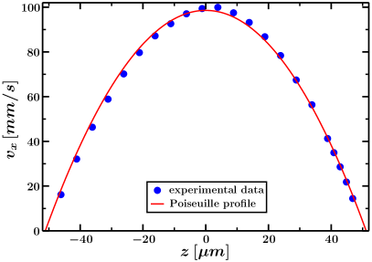
Figure 10: (Color online) Flow profile and Poiseuille fit along $z$-direction (surface of measurement is located at $z\simeq 50\mu m$).

The purpose of this appendix is to analyze the theoretical background of this fit in some more detail. For a pure Poiseuille flow, i. e. a simple parabolic profile, it is clear that the shear rate at the surface does not depend on the slip length $l_{s}$, because in this case a finite $l_{s}$ value simply shifts the profile by a constant amount. Therefore, in this case $l_{s}$ is indeed irrelevant for the fit. A short discussion on such issues is also found in Ref. Lum03 , and experimentally Jos05 ; Vin09 it is also known that typically the shift is so small that a finite slip length is hard to detect by direct measurements of the profile. However, from a theoretical and quantitative point of view it is not quite clear how well it is justified to assume a strictly parabolic profile, i. e. to assume that the flow extends infinitely in $y$ direction — in our experiments, $L_{y}/L_{z}=40$, which is large but not infinite. For finite values of $L_{y}/L_{z}$, the profile is somewhat distorted, and if this distortion is sufficiently large, then also a possible effect of $l_{s}$ should be taken into account. These questions can be easily answered by solving the flow problem in a rectangular channel in the presence of slip exactly, and this shall be done in what follows. The result of this analysis will be that for our conditions the distortion of the profile is indeed completely negligible, and that therefore $l_{s}$ needs not be taken into account either.

We start by considering the Stokes equation

$$\eta\left(\frac{\partial^{2}}{\partial y^{2}}+\frac{\partial^{2}}{\partial z^{2}}\right)v_{x}(y,z)+f=0,$$ (42)

in a rectangular channel with dimensions $[-L_{y}/2,L_{y}/2]\times[-L_{z}/2,L_{z}/2]$ in the $yz$-plane, as in the experiment. Here, $\eta$ is the viscosity of the liquid and $f$ is the driving force density or pressure gradient acting on the liquid in $x$-direction. We assume that all surfaces have the same slip length.

For the case of a no-slip boundary condition, the solution has been given in the textbook of Spurk and Aksel Spu06 , however in a form that does not explicitly spell out the symmetry under exchange of $y$ and $z$. Here we give the solution in a form that shows that symmetry, and generalize it to the case of a nonvanishing slip length $l_{s}$.

Using the methods and notation of quantum mechanics, and allowing for some minor amount of numerics to evaluate a series, the solution is simple and straightforward. We identify a function $f(y,z)$ with a vector $\left|f\right>$ in a Hilbert space, and define the scalar product as

$$\left<f|g\right>=\int_{-L_{y}/2}^{+L_{y}/2}dy\int_{-L_{z}/2}^{+L_{z}/2}dzf^{\star}(y,z)g(y,z).$$ (43)

Defining a “Hamilton operator” via

$${\cal H}=-\frac{\eta}{f}\left(\frac{\partial^{2}}{\partial y^{2}}+\frac{\partial^{2}}{\partial z^{2}}\right),$$ (44)

the Stokes equation is written as

$${\cal H}\left|v_{x}\right>=\left|1\right>.$$ (45)

Obviously, the functions

$$\left|k_{y},k_{z}\right>=N(k_{y},k_{z})\cos(k_{y}y)\cos(k_{z}z)$$ (46)

with $k_{y}>0$, $k_{z}>0$ and

$$N(k_{y},k_{z}) = \left[\frac{L_{y}}{2}+\frac{\sin(k_{y}L_{y})}{2k_{y}}\right]^{-1/2}$$ (47)

$$\times \left[\frac{L_{z}}{2}+\frac{\sin(k_{z}L_{z})}{2k_{z}}\right]^{-1/2}$$

are normalized eigenfunctions of ${\cal H}$,

$${\cal H}\left|k_{y},k_{z}\right>=\frac{\eta}{f}\left(k_{y}^{2}+k_{z}^{2}\right)\left|k_{y},k_{z}\right>$$ (48)

with

$$\left<k_{y},k_{z}|q_{y},q_{z}\right>=\delta_{k_{y},q_{y}}\delta_{k_{z},q_{z}}.$$ (49)

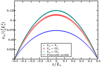
Figure 11: (Color online) One-dimensional cut of the flow profile at $y=0$ for no-slip boundary conditions and several values of $L_{y}$.

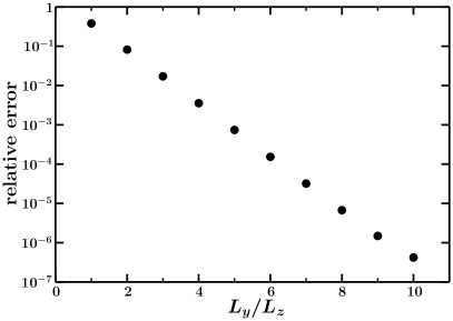
Figure 12: Averaged deviation between a one-dimensional cut of the flow profile at $y=0$ for no-slip boundary conditions and the Poiseuille solution, as function of the width-height ratio of the channel.

The eigenfunctions must satisfy the boundary conditions, and hence the discrete wave numbers $k_{y}$, $k_{z}$ must be the solutions of the transcendental equations

$$l_{s}k_{y} = \cot\left(k_{y}\frac{L_{y}}{2}\right),$$ (50a)

$$l_{s}k_{z} = \cot\left(k_{z}\frac{L_{z}}{2}\right),$$ (50b)

which, in the general case, can be found numerically. In the no-slip case, the solutions are simply given by $k_{y}=\pi/L_{y},3\pi/L_{y},\ldots$ and analogously for $k_{z}$. Equation 50 allows us to re-write Eq. 47 as

$$N(k_{y},k_{z}) = \left[\frac{L_{y}}{2}+l_{s}\sin^{2}\left(k_{y}\frac{L_{y}}{2}\right)\right]^{-1/2}$$ (51)

$$\times \left[\frac{L_{z}}{2}+l_{s}\sin^{2}\left(k_{z}\frac{L_{z}}{2}\right)\right]^{-1/2}.$$

Since the set of eigenfunctions is complete, the spectral representations of ${\cal H}$ and ${\cal H}^{-1}$ are given by

$${\cal H} = \frac{\eta}{f}\sum_{k_{y},k_{z}}\left(k_{y}^{2}+k_{z}^{2}\right)\left|k_{y},k_{z}\right>\left<k_{y},k_{z}\right|,$$ (52)

$${\cal H}^{-1} = \frac{f}{\eta}\sum_{k_{y},k_{z}}\left(k_{y}^{2}+k_{z}^{2}\right)^{-1}\left|k_{y},k_{z}\right>\left<k_{y},k_{z}\right|,$$ (53)

resulting in the solution

$$\left|v_{x}\right> = {\cal H}^{-1}\left|1\right>$$

$$= \frac{f}{\eta}\sum_{k_{y},k_{z}}\left(k_{y}^{2}+k_{z}^{2}\right)^{-1}\left<k_{y},k_{z}|1\right>\left|k_{y},k_{z}\right>$$

$$= \frac{f}{\eta}\sum_{k_{y},k_{z}}\left(k_{y}^{2}+k_{z}^{2}\right)^{-1}N(k_{y},k_{z})^{2}\frac{4}{k_{y}k_{z}}$$

$$\times \sin\left(k_{y}\frac{L_{y}}{2}\right)\sin\left(k_{z}\frac{L_{z}}{2}\right)\cos(k_{y}y)\cos(k_{z}z).$$

Figure 11 shows the resulting flow profile at $y=0$ (in the center of the channel) as a function of $z$, for vanishing slip length and various width-to-height ratios $L_{y}/L_{z}$ of the channel. One sees that the convergence to the asymptotic Poiseuille profile $v_{\mathrm{P}}$ is indeed extremely rapid. The deviation, defined via

$$\mathrm{relative\;error}=\frac{1}{L_{z}}\int_{-L_{z}/2}^{L_{z}/2}dz\left|\frac{v_{x}(0,z)-v_{\mathrm{P}}(z)}{v_{\mathrm{P}}(z)}\right|,$$ (55)

is displayed as a function of $L_{y}/L_{z}$ in Fig. 12. The rate of convergence is apparently exponential, and for the experimental value $L_{y}/L_{z}=40$ the deviation is seen to be much smaller than the resolution of the measurements. Therefore, the assumption of a parabolic profile is indeed justified.

References

- (1) P. Tabeling, Introduction to Microfluidics (Oxford University Press, Oxford, 2006).
- (2) O. I. Vinogradova, International Journal of Mineral Processing 56, 31 (1999).
- (3) J. S. Ellis and M. Thompson, PCCP 6, 4928 (2004).
- (4) C. Neto et al., Rep. Prog. Phys. 68, 2859 (2005).
- (5) E. Lauga, M. P. Brenner, and H. A. Stone, Microfluidics: The No-Slip Boundary Condition, in Handbook of Experimental Fluid Dynamics, J. Foss, C. Tropea, and A. Yarin (Springer, New York, 2007), pp. 1219–1240.
- (6) E. Bonaccurso, M. Kappl, and H.-J. Butt, Phys. Rev. Lett. 88, 076103 (2002).
- (7) C. Neto, V. S. J. Craig, and D. R. M. Williams, Eur. Phys. J. E: Soft Matter Biol. Phys. 12, S71 (2003).
- (8) T. S. Rodrigues, H. J. Butt, and E. Bonaccurso, Colloids and Surfaces A 354, 72 (2010).
- (9) S. Guriyanova and E. Bonaccurso, PCCP 10, 4871 (2008).
- (10) F. Feuillebois, M. Z. Bazant, and O. I. Vinogradova, Phys. Rev. Lett. 102, 026001 (2009).
- (11) D. Einzel, P. Panzer, and M. Liu, Phys. Rev. Lett. 64, 2269 (1990).
- (12) W. A. Ducker, T. J. Senden, and R. M. Pashley, Nature 353, 239 (1991).
- (13) H.-J. Butt, Biophys. J. 60, 1438 (1991).
- (14) O. I. Vinogradova, Langmuir 11, 2213 (1995).
- (15) R. Pit, H. Hervet, and L. Leger, Phys. Rev. Lett. 85, 980 (2000).
- (16) D. C. Tretheway and C. D. Meinhart, Physics of Fluids 14, L9 (2002).
- (17) P. Joseph and P. Tabeling, Phys. Rev. E 71, 035303 (2005).
- (18) P. Huang, J. S. Guasto, and K. S. Breuert, Journal of Fluid Mechanics 566, 447 (2006).
- (19) D. Lasne et al., Phys. Rev. Lett. 100, 214502 (2008).
- (20) C. I. Bouzigues, P. Tabeling, and L. Bocquet, Phys. Rev. Lett. 101, 114503 (2008).
- (21) H. F. Li and M. Yoda, Journal of Fluid Mechanics 662, 269 (2010).
- (22) R. Rigler and E. Elliot, Fluorescence Correlation Spectroscopy: Theory and Applications (Springer, Berlin; New York, 2001).
- (23) D. Magde, W. W. Webb, and E. L. Elson, Biopolymers 17, 361 (1978).
- (24) A. V. Orden and R. A. Keller, Analytical Chemistry 70, 4463 (1998).
- (25) R. H. Kohler, P. Schwille, W. W. Webb, and M. R. Hanson, Journal of Cell Science 113, 3921 (2000).
- (26) M. Gösch et al., Analytical Chemistry 72, 3260 (2000).
- (27) M. Brinkmeier, K. Dörre, J. Stephan, and M. Eigen, Analytical Chemistry 71, 609 (1999).
- (28) P. S. Dittrich and P. Schwille, Analytical Chemistry 74, 4472 (2002).
- (29) D. Lumma et al., Phys. Rev. E 67, 056313 (2003).
- (30) O. I. Vinogradova, K. Koynov, A. Best, and F. Feuillebois, Phys. Rev. Lett. 102, 118302 (2009).
- (31) D. Axelrod, T. P. Burghardt, and N. L. Thompson, Ann. Rev. of Bioph. and Bioeng. 13, 247 (1984).
- (32) K. Hassler et al., Optics Express 13, 7415 (2005).
- (33) J. Ries, E. P. Petrov, and P. Schwille, Biophysical Journal 95, 390 (2008).
- (34) S. Yordanov, A. Best, H. J. Butt, and K. Koynov, Optics Express 17, 21149 (2009).
- (35) W. K. Idol and J. L. Anderson, J. Membrane Sci. 28, 269 (1986).
- (36) C. Cottin-Bizonne, B. Cross, A. Steinberger, and E. Charlaix, Phys. Rev. Lett. 94, 056102 (2005).
- (37) L. Joly, C. Ybert, and L. Bocquet, Phys. Rev. Lett. 96, 046101 (2006).
- (38) C. D. F. Honig and W. A. Ducker, Phys. Rev. Lett. 98, 028305 (2007).
- (39) J. R. Lakowicz, Principles of Fluorescence Spectroscopy, 3rd ed. (Springer, New York, 2006).
- (40) B. Zhang, J. Zerubia, , and J.-C. Olivo-Marin, Appl. Opt. 46, 1819 (2007).
- (41) R. H. Webb, Rep. Prog. Phys. 59, 427 (1996).
- (42) B. Richards and E. Wolf, Proc. R. Soc. A 253, 358 (1959).
- (43) M. Born and E. Wolf, Principles of optics, 7th ed. (Cambridge University Press, Cambridge, 1999).
- (44) D. E. Elrick, Aust. J. Phys. 15, 283 (1962).
- (45) R. T. Foister and T. G. M. Van De Ven, J. Fluid Mech. 96, 105 (1980).
- (46) K. Hassler et al., Biophysical Journal 88, L01 (2005).
- (47) H. Risken, The Fokker–Planck Equation, 2nd ed. (Springer, Berlin Heidelberg New York, 1996).
- (48) J. Honerkamp, Stochastic Dynamical Systems (VCH, New York, 1994).
- (49) H. Öttinger, Stochastic Processes in Polymeric Fluids (Springer, Berlin, 1996).
- (50) R. M. Mazo, Brownian Motion, 1st ed. (Clarendon Press, Oxford, 2002).
- (51) P. Szymczak and A. J. C. Ladd, Phys. Rev. E 68, 036704 (2003).
- (52) D. P. Landau and K. Binder, A Guide to Monte Carlo Simulations in Statistical Physics (Cambridge Univ. Press, Cambridge, 2000).
- (53) B. L. Welch, Biometrika 29, 350 (1938).
- (54) M. Mezard, G. Parisi, and M. A. Virasoro, Spin glass theory and beyond (World Scientific, Singapore, 1987).
- (55) P. Holmqvist, J. K. G. Dhont, and P. R. Lang, J. Chem. Phys. 126, 044707 (2007).
- (56) J. H. Spurk and N. Aksel, Strömungslehre, 6th ed. (Springer, Berlin Heidelberg New York, 2006).