Time dependence of quantum entanglement in the collision of two particles

Abstract

We follow the emergence of quantum entanglement in a scattering event between two initially uncorrelated distinguishable quantum particles interacting via a delta potential. We calculate the time dependence of the Neumann entropy of the one-particle reduced density matrix. By using the exact propagator for the delta potential, we derive an approximate analytic formula for the asymptotic form of the two-particle wave function which is sufficiently accurate to account for the entanglement features of the system.

I Introduction

Quantum entanglement has become an important research topic in modern physics, not only because it exhibits the striking differences from classical concepts, but also since it is widely considered now as the fundamental resource in quantum information theory. Although the first famous paradox connected with entanglement Einstein et al. (1935) was presented in the context of observables with continuous values, the specific entanglement properties of such systems Braunstein and van Loock (2005); Braunstein and Kimble (1998); Hillery (2000); Simon (2000) are less explored than those with discrete, e.g. spin states.

Recent studies of continuous variable quantum systems focus on the emergence of bipartite entanglement in a scattering event of two interacting distinguishable quantum particles, which have no initial correlations Schulman (2004); Tal and Kurizki (2005); Wang et al. (2005, 2006); Busshardt and Freyberger (2007); Law (2004). Since this is a fundamental process in quantum physics, it is important to explore how does it generate quantum entanglement. Some general features of this process were identified in Harshman and Hutton (2008); Harshman and Singh (2008). Refs. Mack and Freyberger (2002); Wang et al. (2005); Busshardt and Freyberger (2007) considered specific models on the scattering of ultracold atoms trapped in a harmonic potential well. Important results on the entanglement of colliding particles, modelled by Gaussian wave packets and interacting with different finite range potentials, were published in Schulman (1998, 2004); Law (2004); Tal and Kurizki (2005); Schmuser and Janzing (2006); Harshman and Singh (2008).

In the present work we consider the explicit time dependence of entanglement in a quantum mechanical model of a collision process which itself creates the entanglement during the interaction between two particles that were independent in the beginning. To be specific, we assume a non-relativistic one dimensional motion with an attractive or repulsive delta potential between the particles. The evolution of the process is described by the explicit solution of the time dependent Schrödinger equation. Although this problem has been considered previously, here we derive analytic expressions for the post collision behaviour that incorporate the spread of the individual wave packets, by using the exact propagator for the delta potential Elberfeld and Kleber (1988); Blinder (1988). To quantify the entanglement we use the Neumann entropy Neumann (1955), and we present how it is built up during the collision. The asymptotic value of the entropy is then obtained from our analytic expression of the long time limit of the time dependent two-particle wave function. This study may find application e.g. in the experimental analysis of collision and recollision of atomic fragments following a laser induced dissociation Kelkensberg et al. (2011).

II Interaction of two particles via a delta potential

The Hamiltonian of the system is written in terms of the position and momentum operators of the particles as

$$H_{12}=\frac{P_{1}^{2}}{2m_{1}}+\frac{P_{2}^{2}}{2m_{2}}-V_{0}\delta\left(X_{1}-X_{2}\right).$$ (1)

For an attractive (repulsive) interaction we have here $V_{0}>0,$ $(V_{0}<0)$. We introduce, as usual for two-body problems, the operators:

$$X_{0} =\alpha_{1}X_{1}+\alpha_{2}X_{2},\qquad P_{0} =P_{1}+P_{2}$$ (2)

$$X =X_{1}-X_{2},\qquad\qquad P =\alpha_{2}P_{1}-\alpha_{1}P_{2}$$ (3)

resulting in a sum of two independent Hamiltonians corresponding to the center of mass motion and the relative motion:

$$H_{12}=H_{0}+H,\qquad H_{0}=\frac{P_{0}^{2}}{2m},\qquad H=\frac{P^{2}}{2\mu}-V_{0}\delta(X).$$ (4)

Here $m=m_{1}+m_{2}$ is the total mass of the particles, $\alpha_{i}=m_{i}/m$   and$\ \mu=m_{1}m_{2}/(m_{1}+m_{2})$ is the reduced mass of the system. In the center of mass reference frame the expectation value of $P_{0}$, the total momentum of the particles, is zero, and the natural coordinate system is the one which has its origin in the expectation value of the center of mass operator, $X_{0}$. Then $\left\langle P_{0}\right\rangle=0$ and $\left\langle X_{0}\right\rangle=0$ for all times. We shall proceed by using coordinate wave functions and assume that initially the particles are described by a product of normalized Gaussians

$$\Psi\left(x_{1},x_{2},t=0\right) = \varphi_{1}(x_{1})\varphi_{2}(x_{2})$$ (5)

$$= \frac{(\alpha_{1}\alpha_{2})^{1/4}}{\sigma\sqrt{\pi}}e^{-\alpha_{1}\left(x_{1}+a_{1}\right)^{2}/2\sigma^{2}}e^{ik_{1}x_{1}}e^{-\alpha_{2}\left(x_{2}-a_{2}\right)^{2}/2\sigma^{2}}e^{ik_{2}x_{2}}$$ (6)

localized at distant points: around $-a_{1}=-\alpha_{2}a$ and $a_{2}=\alpha_{1}a,$ as required by $\left\langle X_{0}\right\rangle=0.$ From $\left\langle P_{0}\right\rangle=0$ we also have $-k_{2}=k_{1}=:q$. In terms of the center of mass and relative coordinates, $x_{0}$ and $x$ this wave function takes the form:

$$\Psi\left(x_{1},x_{2},t=0\right)=\Phi\left(x_{0},x,t=0\right)=\varphi_{c}\left(x_{0}\right)\varphi_{r}\left(x\right),$$ (7)

where

$$\varphi_{c}\left(x_{0}\right) = \sigma^{-1/2}\pi^{-1/4}e^{-x_{0}^{2}/2\sigma^{2}},\qquad$$ (8)

$$\varphi_{r}\left(x\right) = (\alpha/\sigma)^{1/2}\pi^{-1/4}e^{-\alpha^{2}\left(x+a\right)^{2}/2\sigma^{2}}e^{iqx}\qquad$$ (9)

are normalized functions of $x_{0}$ and $x,$ respectively, $a=a_{1}+a_{2}$ is the mean value of the distance between the particles, and $\alpha^{2}=\alpha_{1}\alpha_{2}=\mu/m$.

The separability of the wave function in terms of the coordinates $x$ and $x_{0}$ is due to the specific choice of the initial wave function Schulman (1998, 2004); Schmuser and Janzing (2006); Harshman and Singh (2008); Harshman and Hutton (2008), where the variances of the positions of the individual particles $(\Delta X_{i})^{2}$ obey $m_{1}(\Delta X_{1})^{2}=m_{2}(\Delta X_{2})^{2}$. In the more general case, one has a double sum of products of arbitrary basis functions in the new variables, which could still be transformed into a single sum in the Schmidt bases of the respective spaces (see Eq. (16) below). As implied by the linearity of the Schrödinger equation, the time evolution of the initial state could then be obtained by solving the problem for each term in the sum.

The time evolution of the wave function in the coordinates $x_{0}$ and $x$ are determined by $H_{0}$ and $H$ independently, and they can be given by the respective propagators. For the free motion of the center of mass this is well known:

$$K_{m}^{0}(x_{0},y_{0},t)=\left(\frac{m}{2\pi i\hbar t}\right)^{1/2}\exp\left[im(x_{0}-y_{0})^{2}/2\hbar t\right]$$ (10)

which yields the usual spreading Gaussian wave packet according to:

$$\Phi_{c}\left(x_{0},t\right) =\int K_{m}^{0}(x_{0},y_{0},t)\varphi_{c}(y_{0})dy_{0}=$$ (11)

$$=N_{t}\exp\left[-x_{0}^{2}/2\sigma_{t}^{2}\right]$$

where $N_{t}=\pi^{-1/4}(\sigma+i\hbar t/m\sigma)^{-1/2}$ and $\sigma_{t}^{2}=\sigma^{2}+i\hbar t/m.$ The propagator for the delta potential Hamiltonian is more complicated, but still can be obtained in a closed form. For the attractive case ($V_{0}>0$) the propagator has been derived in Blinder (1988), while it turns out that the result is valid for both signs of the potential and is given by:

$$K(x,y,t)=K_{\mu}^{0}(x,y,t)+\frac{g}{2}e^{-\frac{(|x|+|y|)^{2}}{4\beta}}e^{u^{2}}\mbox{erfc}\left(u\right),$$ (12)

where

$$g=\frac{\mu V_{0}}{\hbar^{2}},\qquad\beta=\frac{i\hbar t}{2\mu},\qquad u=\frac{|x|+|y|}{\sqrt{2i\hbar t/\mu}}-g\sqrt{i\hbar t/2\mu}$$ (13)

The time dependence of the relative wave function can now be given as:

$$\Phi_{r}\left(x,t\right)=\int K(x,y,t)\varphi_{r}(y)dy$$ (14)

It is not possible to determine $\Phi_{r}\left(x,t\right)$ in a closed form given its initial value by (9), we have to rely on numerical integration, but a very good approximate formula, valid for large times, will be given below.

In order to consider the entanglement of the particles one makes the substitution corresponding to (2) and obtains a function of $x_{1}$ and $x_{2}$:

$$\Psi\left(x_{1},x_{2},t\right)=\Phi_{c}\left(x_{0},t\right)\Phi_{r}\left(x,t\right)=\Phi_{c}(\alpha_{1}x_{1}+\alpha_{2}x_{2},t)\Phi_{r}(x_{1}-x_{2},t).$$ (15)

which is not a separable state in the original coordinates $x_{1}$ and $x_{2}$ any more. The above mentioned approximation for $\Phi_{r}\left(x,t\right)$ will enable us to treat $\Psi\left(x_{1},x_{2},t\right)$ analytically, and consider explicitly the entanglement involved in it.

III Reduced density operator and entanglement

In order to quantify entanglement in the state in (15) one uses a measure that characterizes how much an actual two-particle wave function is different from a single product of two one-particle wave functions. In the context of quantum mechanics this was formulated first by J. Neumann Neumann (1955), based on the Schmidt decomposition Schmidt (1907) theorem. It states that for a square integrable function $\Psi(x_{1},x_{2},t)$ of two variables, there exist a set of functions $\phi_{k}(x_{1},t)$ and $\psi_{k}(x_{2},t)$ which both form an orthonormal (but not necessarily complete) set in their respective Hilbert spaces, such that $\Psi$ can be written as a single sum of their products:

$$\Psi(x_{1},x_{2},t)=\sum\limits_{k}\sqrt{p_{k}(t)}\phi_{k}(x_{1},t)\psi_{k}(x_{2},t),$$ (16)

The actual values of the $p_{k}$-s are the simultaneous eigenvalues of the reduced density operators $\hat{\varrho}_{1}$ and $\hat{\varrho}_{2}$ describing either of the two subsystems defined by the hermitian kernel:

$$\varrho_{1}(x_{1}^{\prime},x_{1},t)=\int\Psi^{\ast}(x_{1}^{\prime},x_{2},t)\Psi(x_{1},x_{2},t)dx_{2}$$ (17)

for system 1 and similarly for system 2. As it is shown in Neumann (1955); Schmidt (1907) in more detail, $\hat{\varrho}_{1}$ and $\hat{\varrho}_{2}$ have a complete set of square integrable eigenfunctions forming a basis, $\phi_{k}(x_{1})$, $\psi_{k}(x_{2})$ respectively, such that the corresponding eigenvalues $p_{k}$ are identical. The $p_{k}$-s are nonnegative and form a discrete set, the sum of which is equal to unity. This also implies that the multiplicity of a positive eigenvalue must be finite.

For quantifying entanglement it is natural to use the measure of randomness of the discrete probability distribution given by the $p_{k}$-s in the Schmidt sum. Statistical physics tells us that this is best characterized by $S=-\sum\limits_{k}p_{k}\ln p_{k}$, which is just the Neumann entropy belonging to the reduced density operator for each of the particles

$$S(t)=-\mbox{Tr}\left[\hat{\rho}_{1}(t)\ln\hat{\rho}_{1}(t)\right]=-\mbox{Tr}\left[\hat{\rho}_{2}(t)\ln\hat{\rho}_{2}(t)\right]$$ (18)

In order to calculate $S$ one has to find the nonzero eigenvalues $p_{k}$, that shall be time dependent during the collision. Fig. 1 shows numerical results about the time dependence of the quantum entanglement during the collision process, using atomic units.

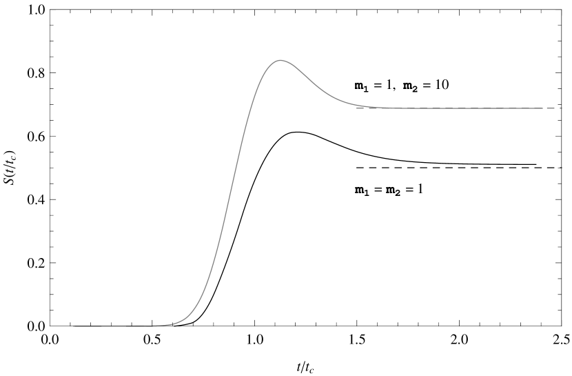
Figure 1: Time dependence of the quantum entanglement during the collision process. We plot the Neumann entropy (18), computed numerically, vs. time measured in units of the classical collision time $t_{c}=ma/\hbar q$. The black solid curve is for $m_{1}=m_{2}=1$, while the gray solid curve is for $m_{1}=1$, $m_{2}=10$, as indicated in the figure. The dashed lines mark the asymptotic values of $S$, given by formula (28). We use atomic units, the parameters are: $V_{0}=-5,\,a=10,\,q=5,\,\sigma=1/2$.

IV Approximate propagator and entropy for long times

The time evolution of the relative wave function, i.e. the second factor in (14) cannot be given in a closed form. We find an approximate analytical formula for the relative wave function and entropy using certain approximations for the propagator given by (12).

The assumption that initially the particles are localized  in a large distance from each other means that $\varphi_{r}(y)$ is different from zero only around $-a\ll 0$, therefore the contribution to the integral in (14) for $y>0$ can be neglected, and $|y|$ can be replaced by $-y$ in the propagator (12). Setting $v=\hbar q/m,$ which is the mean velocity of the relative wave packet, we can consider the asymptotic behaviour of the system for times much larger than $t_{c}=a/v$, which is the time instant of the corresponding classical collision. We can use then the asymptotic approximation Abramowitz and Stegun (1965): $\exp(u^{2})\mbox{erfc}(u)=(\sqrt{\pi}\,{u})^{-1}(1-{u^{-2}}/2+O({u^{-4}}))$, valid for large values of $u$. Keeping only the first term here we have then:

$$K=K_{0}^{\mu}+K_{1}^{\mu}= (4\pi\beta)^{-1/2}\exp\left[-\frac{(x-y)^{2}}{4\beta}\right]+$$ (19)

$$\frac{g\sqrt{\beta}}{\sqrt{\pi}\left(|x|-y-2g\beta\right)}\exp\left[-\frac{(|x|-y)^{2}}{4\beta}\right].$$

The reduced (one-particle) density matrix in the form of Eq. (17) cannot be calculated from the propagator (19) analytically. Therefore, we simplify it further by replacing the $x$ and $y$ variables of the propagator with the classical initial and final coordinate values, $y=-a$ and $|x|=|-a+\hbar qt/\mu|$, in the prefactor of the exponential of $K_{1}$, but keeping the position dependence in the rapidly oscillating phase factor. This approximation is similar to the usual one in scattering theory, and yields the propagator

$$K(x,y,t) = (4\pi\beta)^{-1/2}\left(\exp\left[-\frac{(x-y)^{2}}{4\beta}\right]\right.$$ (20)

$$\left.+\left(\frac{|-a+\hbar qt/\mu|+a}{it\hbar g/\mu}-1\right)^{-1}\exp\left[-\frac{(|x|-y)^{2}}{4\beta}\right]\right).$$

Due to the presence of $|x|$ in the exponential of the second term, the integral (14) with the function $\varphi_{r}(y)$ from (9) will split into two distinct Gaussians: one centered around $x=-a+vt$, this corresponds to the forward scattered wave, while the other around $a-vt$  yielding the reflected wave. In this way we get the following asymptotic form of the relative propagator:

$$K(x,y,t)=\sqrt{\frac{\mu}{2\pi i\hbar t}}\left(c_{+}\,\exp\left[\frac{i\mu(x-y)^{2}}{2\hbar t}\right]+c_{-}\,\exp\left[\frac{i\mu(x+y)^{2}}{2\hbar t}\right]\right)$$ (21)

where $c_{-}=\left(\frac{|-a+vt|+a}{i\hbar tg/\mu}-1\right)^{-1}$, $c_{+}=1+c_{-}$. It is easy to check that for times larger than $v/a$ these amplitudes coincide with the plane wave transmission and reflection coefficients for a delta potential with wave number $q,$ which is the mean value of $k$ in the initial relative state:

$$\lim_{t\rightarrow\infty}c_{+}=T(q):=q/(q-ig),\qquad\lim_{t\rightarrow\infty}c_{-}=R(q):=ig/(q-ig)$$ (22)

The great advantage of the approximate form in (21) is that it allows one to proceed entirely analytically and determine the total wave function, as well as the final value of the entanglement entropy in the system in a closed form. This is due to the emergence of Gaussian type integrals in (14), which leads us to the approximate relative wave function

$$\tilde{\Phi}_{r}(x,t)=T(q)\phi_{+}(x,t)+R(q)\phi_{-}(x,t)$$ (23)

where

$$\phi_{\pm}(x,t)=N_{t}\sqrt{\alpha}\exp\left[-\frac{\alpha^{2}(\pm x+a-vt)^{2}}{2(\sigma^{2}+i\hbar t/m)}\right].$$ (24)

The total two-particle wave function is now obtained with Eq. (15), and after some algebra we obtain the result

$$\Psi(x_{1},x_{2},t)=\left[T(q)\Phi_{1}(x_{1},t)\Phi_{2}(x_{2},t)+R(q)\Phi_{1}(-x_{1},t)\Phi_{2}(-x_{2},t)\right]$$ (25)

with

$$\Phi_{j}(\xi,t)=N_{t}\alpha_{j}^{1/4}\exp\left[-\frac{\alpha_{j}(\xi-u_{1}t+a_{j})^{2}+i\gamma_{j}(\xi,t)}{\sigma_{t}^{2}}\right]$$ (26)

and

$$\gamma_{j}(\xi,t)=\frac{\hbar t}{m\sigma^{2}}[\alpha_{j}(a_{j}+\xi)^{2}-\alpha^{2}a^{2}/2]+\sigma^{2}q[2(a_{j}+\xi)-vt/2]$$ (27)

Here $a_{1}=\alpha_{2}a$, $a_{2}=\alpha_{1}a$, the $\sigma_{t}^{2}/\alpha_{j}=(\sigma^{2}+\hbar^{2}t^{2}/\sigma^{2}m^{2})/\alpha_{j}$ describes the spreading of the respective wave packets, and $u_{j}=\hbar q/m_{j}$ are the velocities of the particles in the corresponding classical problem.

Fig. 2 shows $\Phi_{1}(x_{1},t)$ and $\Phi_{1}(-x_{1},t)$ in comparison with the two eigenstates of the computed one-particle density matrix, having the largest eigenvalues.

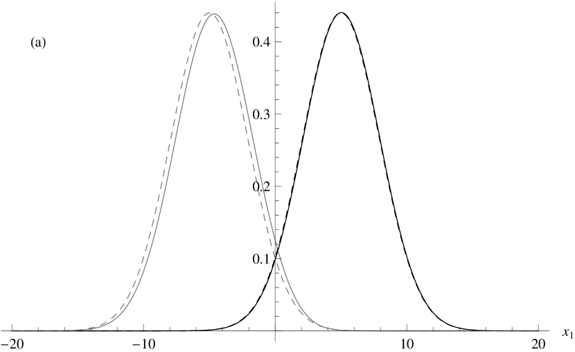
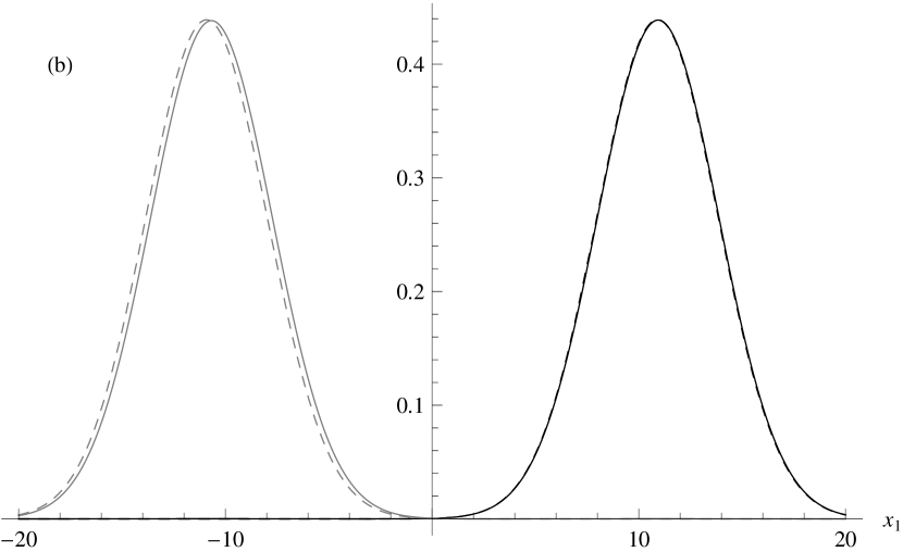
Figure 2: Comparison of the asymptotic analytical results of the Schmidt decomposition, Eq. (25), with the numerical method, for the case of (a) $m_{1}=m_{2}=1$, at $t=2\,t_{c}$, and (b) $m_{1}=1$, $m_{2}=10$, at $t=2\,t_{c}$. We plot the absolute value of the two eigenstates of the one-particle density matrix having the two largest eigenvalues, obtained numerically, with solid black (on the right side) and solid gray (on the left side) curves. The dashed black and dashed gray curves are the absolute values of $\Phi_{1}(x_{1},t)$ and $\Phi_{1}(-x_{1},t)$ functions, respectively, see Eq. (26). We use atomic units, the parameters are: $V_{0}=-5,\,a=10,\,q=5,\,\sigma=1/2$.

The expression (25) is the required approximation of the Schmidt decomposition, consisting of the two terms. The asymptotic value of the entropy of this entangled state is then

$$S =-|T(q)|^{2}\ln|T(q)|^{2}-|R(q)|^{2}\ln|R(q)|^{2}=$$ (28)

$$=-(\frac{q^{2}}{q^{2}+g^{2}}\ln\frac{q^{2}}{q^{2}+g^{2}}+\frac{g^{2}}{q^{2}+g^{2}}\ln\frac{g^{2}}{q^{2}+g^{2}})$$

The entanglement will be maximal for $q=|g|$, i.e. for center of mass momenta with $-p_{2}=p_{1}=\mu|V_{0}|/\hbar$, and has the value $\ln 2$. This explains why we have a larger entanglement for $m_{2}=10m_{1}$, when this condition is almost satisfied.

V Conclusions

We have followed the emergence of the entanglement of two colliding particles that are independent initially and thus their wave function is a product state. In the case of the delta interaction potential and Gaussian initial states we have found an approximate analytic expression for the final entangled state, which is in good agreement with numerical results based on the exact propagator. Let us note that the wave function $\Psi(x_{1},x_{2},t)$ is a kind of an EPR state Einstein et al. (1935) in its original sense, i.e. in the coordinate space of two entangled particles. In Einstein et al. (1935) however the state considered is given by a highly singular delta function, while here $\Psi\left(x_{1},x_{2},t\right)$ is square integrable during the whole process and has an especially simple asymptotic form.

References

References

- Einstein et al. (1935) A. Einstein, B. Podolsky, and N. Rosen, Phys. Rev. 47, 777 (1935).
- Braunstein and van Loock (2005) S. Braunstein and P. van Loock, Rev. Mod. Phys. 77, 513 (2005).
- Braunstein and Kimble (1998) S. Braunstein and H. Kimble, Phys. Rev. Lett. 80, 869 (1998).
- Hillery (2000) M. Hillery, Phys. Rev. A 61, 022309 (2000).
- Simon (2000) R. Simon, Phys. Rev. Lett. 84, 2726 (2000).
- Schulman (2004) L. Schulman, Phys. Rev. Lett. 92, 210404 (2004).
- Tal and Kurizki (2005) A. Tal and G. Kurizki, Phys. Rev. Lett. 94, 160503 (2005).
- Wang et al. (2005) J. Wang, C. Law, and M. Chu, Phys. Rev. A 72, 022346 (2005).
- Wang et al. (2006) J. Wang, C. Law, and M. Chu, Phys. Rev. A 73, 034302 (2006).
- Busshardt and Freyberger (2007) M. Busshardt and M. Freyberger, Phys. Rev. A 75, 052101 (2007).
- Law (2004) C. Law, Phys. Rev. A 70, 062311 (2004).
- Harshman and Hutton (2008) N. L. Harshman and G. Hutton, Phys. Rev. A 77, 042310 (2008).
- Harshman and Singh (2008) N. L. Harshman and P. Singh, J. Phys. A-Math. Theor. 41, 155304 (2008).
- Mack and Freyberger (2002) H. Mack and M. Freyberger, Phys. Rev. A 66, 042113 (2002).
- Schulman (1998) L. S. Schulman, Phys. Rev. A 57, 840 (1998).
- Schmuser and Janzing (2006) F. Schmuser and D. Janzing, Phys. Rev. A 73, 052313 (2006).
- Elberfeld and Kleber (1988) W. Elberfeld and M. Kleber, Am. J. Phys. 56, 154 (1988).
- Blinder (1988) S. M. Blinder, Phys. Rev. A 37, 973 (1988).
- Neumann (1955) J. Neumann, Mathematical Foundations of Quantum Mechanics (Princeton University Press, Princeton, 1955).
- Kelkensberg et al. (2011) F. Kelkensberg et al., Phys. Rev. Lett. 107, 043002 (2011).
- Schmidt (1907) E. Schmidt, Math. Ann. 63, 43 (1907).
- Abramowitz and Stegun (1965) M. Abramowitz and I. Stegun, eds., Handbook of mathematical functions (Dover Publications, New York, 1965).