Stable Graphical Model Estimation with Random Forests for Discrete, Continuous, and Mixed Variables

Abstract

A conditional independence graph is a concise representation of pairwise conditional independence among many variables. Graphical Random Forests (GRaFo) are a novel method for estimating pairwise conditional independence relationships among mixed-type, i.e. continuous and discrete, variables. The number of edges is a tuning parameter in any graphical model estimator and there is no obvious number that constitutes a good choice. Stability Selection helps choosing this parameter with respect to a bound on the expected number of false positives (error control).

The performance of GRaFo is evaluated and compared with various other methods for $p=50$, $100$, and $200$ possibly mixed-type variables while sample size is $n=100$ ($n=500$ for maximum likelihood). Furthermore, GRaFo is applied to data from the Swiss Health Survey in order to evaluate how well it can reproduce the interconnection of functional health components, personal, and environmental factors, as hypothesized by the World Health Organization’s International Classification of Functioning, Disability and Health (ICF). Finally, GRaFo is used to identify risk factors which may be associated with adverse neurodevelopment of children who suffer from trisomy 21 and experienced open-heart surgery.

GRaFo performs well with mixed data and thanks to Stability Selection it provides an error control mechanism for false positive selection.

1 Introduction

In many problems one is not confined to one response and a set of predefined predictors. In turn, the interest is often in the association structure of a whole set of $p$ variables, i.e. asking whether two variables are independent conditional on the remaining $p-2$ variables. A conditional independence graph (CIG) is a concise representation of such pairwise conditional independence among many possibly mixed, i.e. continuous and discrete, variables. In CIGs, variables appear as nodes, whereas the presence (absence) of an edge among two nodes represents their dependence (independence) conditional on all other variables. Applications include among many others also the study of functional health (Strobl et al., 2009; Kalisch et al., 2010; Reinhardt et al., 2011).

We largely focus on the high-dimensional case where the number of variables (nodes in the graph) $p$ may be larger than sample size $n$. A popular approach to graphical modeling is based on the Least Absolute Shrinkage and Selection Operator (LASSO; Tibshirani, 1996): see Meinshausen and Bühlmann (2006) or Friedman et al. (2008) for the Gaussian case and Ravikumar et al. (2010) for the binary case. However, empirical data often involve both discrete and continuous variables. Conditional Gaussian distributions were suggested to model such mixed-type data with maximum likelihood inference (Lauritzen and Wermuth, 1989), but no corresponding high-dimensional method has been suggested yet. Dichotomization, though always applicable, comes at the cost of lost information (MacCallum et al., 2002).

Tree-based methods are easy to use and accurate for dealing with mixed-type data (Breiman et al., 1984). Random Forests (Breiman, 2001) evaluate an ensemble of trees often resulting in notably improved performance compared to a single tree (see also Amit and Geman, 1997). Furthermore, permutation importance in Random Forests allows to rank the relevance of predictors for one specific response. However, Random Forests have also been criticized to perform possibly biased variable selection. We thus also consider Conditional Forests (Strobl et al., 2007) and conditional variable importance (Strobl et al., 2008), which have been suggested to overcome this behavior.

In general, the definition of both the conditional and marginal permutation importance differ for discrete and continuous responses. Thus, ranking permutation importances across responses of mixed-type is less obvious. However, such ranking is essential to derive a network of the most relevant dependencies. Stability Selection proposed by Meinshausen and Bühlmann (2010) is one possible framework to rank the edges in the CIG across different types of variables. In addition, it allows to specify an upper bound on the expected number of false positives, i.e. the falsely selected edges, and thus provides a means of error control.

We combine Random Forests estimation with appropriate ranking among mixed-type variables and error control from Stability Selection. We refer to the new method as Graphical Random Forests (GRaFo). The specific aims of the paper are a) to evaluate and compare the performance of GRaFo with Stable LASSO (StabLASSO) and Stable Conditional Forests (StabcForests), which are LASSO- and conditional forest-based alternatives, and regular maximum likelihood (ML) estimation across various simulated settings comprising different distributions, interactions, and nonlinear associations for $p=50$, $100$, and $200$ possibly mixed-type variables while sample size is $n=100$ ($n=500$ for ML), b) to apply GRaFo to data from the Swiss Health Survey (SHS) to evaluate the interconnection of functional health components, personal, and environmental factors, as hypothesized by the World Health Organization’s (WHO) International Classification of Functioning, Disability and Health (ICF), and c) to use GRaFo to identify risk factors associated with adverse neurodevelopment in children with trisomy 21 after open-heart surgery and more generally to assess the plausibility of the suggested associations.

2 Graphical Modeling Based on Regression-Type Methods

2.1 Conditional Independence Graphs

Let ${\bf X}=\{X_{1},\ldots,X_{p}\}$ be a set of (possibly) mixed-type random variables. The associated conditional independence graph of $\bf X$ is the undirected graph $G_{\mbox{\tiny CIG}}=(\mathcal{V},\mathcal{E}(G_{\mbox{\tiny CIG}}))$, where the nodes in $\mathcal{V}$ correspond to the $p$ variables in ${\bf X}$. The edges represent the pairwise Markov property, i.e. $i-j\not\in\mathcal{E}(G_{\mbox{\tiny CIG}})$ if and only if $X_{j}\mathchoice{\mathrel{\hbox to0.0pt{$\displaystyle\perp$\hss}\mkern 2.0mu{\displaystyle\perp}}}{\mathrel{\hbox to0.0pt{$\textstyle\perp$\hss}\mkern 2.0mu{\textstyle\perp}}}{\mathrel{\hbox to0.0pt{$\scriptstyle\perp$\hss}\mkern 2.0mu{\scriptstyle\perp}}}{\mathrel{\hbox to0.0pt{$\scriptscriptstyle\perp$\hss}\mkern 2.0mu{\scriptscriptstyle\perp}}}X_{i}|{\bf X}\setminus\{X_{j},X_{i}\}$. For a rigorous introduction to graphical models, see, for example, the monographs by Whittaker (1990) or Lauritzen (1996).

We will now show that the pairwise Markov property can, under certain conditions, be inferred from conditional mean estimation.

Theorem 1.

Assume that, for all $j=1,\ldots,p$, the conditional distribution of $X_{j}$ given $\{X_{h};h\neq j\}$ is depending on any realization $\{x_{h};h\neq j\}$ only through the conditional mean function

$$m_{j}(\{x_{h};h\neq j\})=\mathbb{E}[X_{j}|\{x_{h};h\neq j\}],$$

that is:

$$\mathbb{P}[X_{j}\leq x_{j}|\{x_{h};h\neq j\}]=F_{j}(x_{j}|m_{j}(\{x_{h};h\neq j\})),$$ (A)

where $F_{j}(\cdot|m)$ is a cumulative distribution function for all $m\in\mathbb{R}$ (or $m\in\mathbb{R}^{d}$ if $X_{j}$ is $d$-dimensional). (Thereby, we assume that the conditional mean exists). Then

$$X_{j}\mathchoice{\mathrel{\hbox to0.0pt{$\displaystyle\perp$\hss}\mkern 2.0mu{\displaystyle\perp}}}{\mathrel{\hbox to0.0pt{$\textstyle\perp$\hss}\mkern 2.0mu{\textstyle\perp}}}{\mathrel{\hbox to0.0pt{$\scriptstyle\perp$\hss}\mkern 2.0mu{\scriptstyle\perp}}}{\mathrel{\hbox to0.0pt{$\scriptscriptstyle\perp$\hss}\mkern 2.0mu{\scriptscriptstyle\perp}}}X_{i}|\{X_{h};h\neq j,i\}$$

if and only if

$$m_{j}(\{x_{h};h\neq j\})=m_{j}(\{x_{h};h\neq j,i\})$$

does not depend on $x_{i}$, for all $\{x_{h};h\neq j\}$.

A proof is given in Section 8. Assumption $(A)$ trivially holds for a Bernoulli random variable $X_{j}$:

$$\mathbb{P}[X_{j}=1|\{x_{h};h\neq j\}]=\mathbb{E}[X_{j}|\{x_{h};h\neq j\}]=m_{j}(\{x_{h};h\neq j\}).$$

Analogously, for a multinomial random variable $X_{j}$ with $C$ levels, the probability that $X_{j}$ takes the level $r\in\{1,\ldots,C\}$ can be expressed via a Bernoulli variable $X_{j}^{(r)}$ with

$$\mathbb{P}[X_{j}^{(r)}=1|\{x_{h};h\neq j\}]=\mathbb{E}[X_{j}^{(r)}|\{x_{h};h\neq j\}]=m_{j}(\{x_{h};h\neq j\}).$$

Hence, $(A)$ holds. Moreover, if $(X_{1},\ldots,X_{p})\sim\mathcal{N}_{p}({\bf 0},{\bf\Sigma})$, then $(A)$ holds as well (see for example Lauritzen, 1996). However, for the Conditional Gaussian distribution (or CG distribution, see e.g. Lauritzen, 1996), we need to require for $(A)$ that the variance is fixed and is not depending on the variables we condition on. For example, let $X_{1}\sim\mathcal{B}(1,\pi)$ be Bernoulli distributed and let

$$X_{2}|X_{1}\sim\left\{\begin{matrix}\mathcal{N}(\mu_{1},\sigma_{1}^{2}),\mbox{ if }X_{1}=1\\ \mathcal{N}(\mu_{2},\sigma_{2}^{2}),\mbox{ if }X_{1}=0\end{matrix}\right.,\mbox{ where }\sigma_{1}^{2}\neq\sigma_{2}^{2}.$$

Then the distribution of $X_{2}|X_{1}$ is not a function of the conditional mean alone.

Theorem 1 motivates our approach to infer conditional dependences, or edges in the CIG, via variable selection for many nonlinear regressions, i.e. determining whether a variable $X_{i}$ is relevant in $\mathbb{E}[X_{j}|{\bf X}\setminus\{X_{j}\}]$ (regression of $X_{j}$ versus all other variables).

2.2 Ranking Edges

In order to determine which edges should be included in the graphical model, the edges suggested by the individual regressions need to be ranked such that a smaller rank indicates a better candidate for inclusion. Note that each edge $i-j$ is associated with two coefficients ($X_{j}$ regressed on $X_{i}$ and all other variables and vice versa for $X_{i}$ on $X_{j}$). To be conservative, we rank each edge $i-j$ relative to the smaller one of the two (absolute-valued) ranking coefficients.

If variables are mixed-type, a global ranking criterion is difficult to find. For example, continuous and categorical response variables are not directly comparable. Instead, local rankings for each regression are performed separately (where “local” means that we can rank the importance of predictors for every individual regression). Analogous to global ranking, each edge $i-j$ is associated with two possible ranks and the worse among them is used.

When using Random Forests for performing the individual nonlinear regressions, the ranking scheme is obtained from Random Forests’ variable importance measure. For Conditional Forests, both the conditional and marginal variable importances can be used. When using the LASSO for individual linear or logistic regressions, the ranking scheme is obtained from the value of the penalty parameter $\lambda$ for which an estimated regression coefficient first becomes non-zero (i.e. the value of the penalty parameter when a variable enters in a coefficient path plot).

We then have to decide on the number of edges to select, i.e. the tuning parameter. Say it is given as $q=11$. Then, for both global and local rankings, we select the $11$ best-ranked edges across all $p$ individual regressions. If this is impossible due to tied ranks (e.g. because the 11th and 12th best edges have a tied rank of 11.5), we neglect these (here: two) tied edges and select only the remainder of (here: 10) edges not in violation of the tuning parameter.

We next outline how Stability Selection can be used to guide the choice of $q$.

2.3 Aggregating Edge Ranks with Stability Selection

Stability Selection (Meinshausen and Bühlmann, 2010) allows the specification of an upper bound on the expected number $\mathbb{E}[V]$ of false positives. It is based on subsampling (Politis et al., 1999; Bühlmann and Yu, 2002) random subsets ${\bf X}^{(1)},\ldots,{\bf X}^{(n_{\mbox{\tiny sub}})}$ of the original sample ${\bf X}_{1},\ldots,{\bf X}_{n}$, where each ${\bf X}^{(k)}$ contains $\lfloor n/2\rfloor$ sample points.

Let $\mathcal{E}(\hat{G}_{\mbox{\tiny CIG}}({\bf X}^{(k)}))$ denote the edges from a thresholded ranking based on ${\bf X}^{(k)}$, $k=1,\ldots,n_{\mbox{\tiny sub}}$. Stability Selection suggests to construct $\mathcal{E}(\hat{G}_{\mbox{\tiny CIG}}({\bf X}))$, the set of all edges in the estimated CIG of ${\bf X}$, from all edges that were “sufficiently stable” across the $n_{\mbox{\tiny sub}}$ subsets. More concretely, we choose only edges $i-j$ which fulfill

$$\frac{1}{n_{\mbox{\tiny sub}}}\sum_{k=1}^{n_{\mbox{\tiny sub}}}I_{\{i-j\in\mathcal{E}(\hat{G}_{\mbox{\tiny CIG}}({\bf X}^{(k)}))\}}\geq\pi_{\mbox{\tiny thr}},$$ (1)

where $\pi_{\mbox{\tiny thr}}$ imposes a threshold on the minimum relative frequency of edges across the $n_{\mbox{\tiny sub}}$ subsets to be included in $\mathcal{E}(\hat{G}_{\mbox{\tiny CIG}}({\bf X}))$ and $I$ is the indicator function.

In their Theorem 1, Meinshausen and Bühlmann (2010) relate $\mathbb{E}[V]$ to the maximum number of selected edges $q$ per subset, the number of possible edges $p\cdot(p-1)/2$ in $\mathcal{E}(\hat{G}_{\mbox{\tiny CIG}}({\bf X}))$, and the threshold $\pi_{\mbox{\tiny thr}}$ from formula (1) (requiring $\pi_{\mbox{\tiny thr}}\in\left(\frac{1}{2},1\right)$):

$$\mathbb{E}[V]\leq\frac{q^{2}}{(2\pi_{\tiny\mbox{thr}}-1)\cdot p\cdot(p-1)/2}.$$ (2)

The expected number of false positives $\mathbb{E}[V]$, which is a type I error measure, needs to be specified a priori. The parameters $\pi_{\mbox{\tiny thr}}$ and $q$ are tuning parameters that depend on each other. More precisely, to obtain a stable graph estimate for a given $\mathbb{E}[V]$, the threshold $\pi_{\mbox{\tiny thr}}$ has to be large if the number of selected edges $q$ is large and vice versa. Consequently (and as also argued by Meinshausen and Bühlmann, 2010) the actual values of $\pi_{\mbox{\tiny thr}}$ and $q$ are of minor importance for a given $\mathbb{E}[V]$ as the graph estimates do not vary much for different choices of $\pi_{\mbox{\tiny thr}}$ (results not shown). We thus fix $\pi_{\mbox{\tiny thr}}=0.75$ throughout the paper. Also, we follow the suggestion of Meinshausen and Bühlmann (2010) in choosing $n_{\mbox{\tiny sub}}=100$.

We can then use formula (2) to derive

$$q=\lfloor\sqrt{(2\pi_{\mbox{\tiny thr}}-1)\mathbb{E}[V]\cdot p\cdot(p-1)/2}\rfloor$$

by specifying the value of $\mathbb{E}[V]$ as desired (according to the willingness to accept false positives).

Note that formula (2) is based on two assumptions: 1) the estimation procedure is better than random guessing and 2) the probability of a false edge to be selected is exchangeable; for details we refer to Meinshausen and Bühlmann (2010). Also note that $\pi_{\mbox{\tiny thr}}$ is not to be interpreted as an edge probability threshold but solely as a means to assess stability which allows control of $\mathbb{E}[V]$. Finally, be aware that our method does not consider the goodness-of-fit of the model but instead leads to an undirected graph whose edges are controlled for false positive selections.

3 Random Forests, Conditional Forests, LASSO Regression, and Maximum Likelihood

3.1 Random Forests

Random Forests have, to date, not been used to estimate CIGs. They perform a series of recursive binary partitions of the data and construct the predictions from terminal nodes. Based on classification and regression trees (Breiman et al., 1984) they allow convenient inference for mixed-type variables, also in the presence of interaction effects. Incorporating bootstrap (Efron, 1979; Breiman, 1996) and random feature selection (Amit and Geman, 1997), random subsets of both the observations and the predictors are considered. The relevance of each predictor can be assessed with permutation importance (Breiman, 2002), a measure of the error difference between a regular Random Forests fit and a Random Forests fit within which one predictor has been permuted at random to purge its relationship with the response. An implementation of Random Forests in R (R Development Core Team, 2011) is available in the randomForest package (Liaw and Wiener, 2002). We chose the number of trees and the number of features randomly selected per tree according to the package defaults. Further extensions (which we did not incorporate) allow to explicitly use the ordinal information of a categorical response: see e.g. the R packages party (Hothorn et al., 2006) and rpartOrdinal (Archer, 2010).

Since the goodness-of-fit of continuous and categorical responses is based on mean squared errors and majority votes, respectively, the goodness-of-fit and importance measures are not directly comparable across mixed-type responses. Thus a local ranking is derived, where each edge $i-j$ is assigned either the rank of the permutation importance of predictor $X_{i}^{(k)}$ for response $X_{j}^{(k)}$ or of predictor $X_{j}^{(k)}$ for response $X_{i}^{(k)}$ (whichever is more conservative, i.e. assigns a worse rank) and finally aggregated with Stability Selection; the upper index ^(k) denotes the $k^{th}$ subsample in Stability Selection. We refer to this procedure as Graphical Random Forests (GRaFo) henceforth.

3.2 Conditional Forests

Strobl et al. (2007) criticized Random Forests to favor variables with many categories. Furthermore, Random Forests have been criticized to favor correlated predictors, even if not all of them are influential for the response (Strobl et al., 2008).

To overcome the first limitation, Conditional Forests (Strobl et al., 2007) were suggested, which are a modification of the original Random Forests implementation. They are based on conditional inference trees (Hothorn et al., 2006), an unbiased tree learning procedure, to obtain an unbiased ensemble of trees.

While the regular marginal permutation importance discussed in the previous section is also applicable to Conditional Forests, a conditional permutation importance, which aims to preserve the correlation structure among predictors, has been suggested by Strobl et al. (2008) to overcome the latter critique of forest ensembles favoring correlated predictors. An implementation of Conditional Forests, including the conditional variable importance, is available in the party package (Hothorn et al., 2006) in R. However, we found that the computational cost to obtain the conditional variable importance is a lot higher than for the marginal permutation importance. When drastically reducing the number of trees to 10, the computations become feasible but the ensemble does hardly produce any true positives (likely due to instability of the small forest ensemble). As such, all calculations reported further below have been performed using the marginal permutation importance. To allow a fair comparison, we set the ensemble size to 500 trees (as with Random Forests).

The same ranking rule as for Random Forests can then be used to construct a Stable Conditional Forest (StabcForests) algorithm.

3.3 Least Absolute Shrinkage and Selection Operator (LASSO)

In the case of linear regression for continuous responses and predictors, the LASSO (Tibshirani, 1996) penalizes with the $\ell_{1}$-norm and corresponding penalty parameter $\lambda$ the coefficients of some less relevant predictors to zero. The larger $\lambda$ is chosen, the more coefficients will be set to zero. This concept has also been extended to logistic regression (Lokhorst, 1999) and implemented in R in the glmnet package (Friedman et al., 2010). In the case of multinomial and mixed-type data, no eligible off-the-shelf implementation of the LASSO is available. We hence dichotomize these data according to a median split for continuous variables and aggregate categories such that the resulting frequency of the -1 and 1 categories was as balanced as possible for discrete variables. Consequently, a loss of information is to be expected (cf., MacCallum et al., 2002; Altman and Royston, 2006; Royston et al., 2006).

CIG estimation via the LASSO with Stability Selection was suggested for Gaussian data by Meinshausen and Bühlmann (2010) and can be represented as a global ranking. For each response $X_{j}^{(k)}$, we estimate LASSO regressions with all remaining ${\bf X}^{(k)}\setminus\{X_{j}^{(k)}\}$ as predictors and with a decreasing sequence of penalties $\lambda_{j}^{(k),\mbox{\tiny max}},\ldots,\lambda_{j}^{(k),\mbox{\tiny min}}$. Let $\lambda_{ij}^{(k)}$ denote the largest penalty value of the sequence for which the coefficient of predictor $X_{i}^{(k)}$ for response $X_{j}^{(k)}$ is non-zero, and if no such penalty exists let $\lambda_{ij}^{(k)}=0$. For each edge $i-j$ we select the more conservative penalty $\lambda_{i-j}^{(k)}=\min\left(\lambda_{ij}^{(k)},\lambda_{ji}^{(k)}\right)$ and rank $i-j$ relative to the global rank from the absolute-valued estimated regression coefficient corresponding to $\lambda_{i-j}^{(k)}$. As before, the upper index ^(k) denotes the $k^{th}$ subsample from Stability Selection. We denote this procedure in combination with Stability Selection as Stable LASSO (StabLASSO).

3.4 Maximum Likelihood

Ordinary maximum likelihood (ML) estimation does neither impose a penalty (such as the LASSO) nor does it use subsampling to reduce the number of predictors to consider in each run (such as the Forest-type algorithms). Consequently, ordinary ML inference can only be applied in the case, where the number of parameters to be estimated is at most as large as the sample size $n$.

If the dependent variable is continuous, we use the ordinary linear model, otherwise the multinomial log-linear model. Local rankings are obtained from the F-Test for each of the predictor variables. The calculations were performed with the regr0 package (available from R-Forge) in R.

We could wrap a Stability Selection scheme around ML estimation which is computationally demanding in the case of mixed continuous and categorical variables. Our main goal here, however, is to compare with plain ML estimation.

4 Simulation Study

4.1 Simulating Data from Directed Acyclic Graphs

We use a directed acyclic graph (DAG; cf., Whittaker, 1990) to embed conditional dependence statements among nodes representing the $p$ random variables. The associated CIG follows by moralization, i.e. connecting any two parents with a common child that are not already connected and removing all arrowheads (Lauritzen and Spiegelhalter, 1988).

Let $\mathcal{A}$ be a $(p\times p)$-dimensional weight matrix with entries $a_{ij}\in\{[-1,-0.1]\cup\{0\}\cup[0.1,1]\}$ if $i<j$ and $a_{ij}=0$ otherwise. In addition, we sample $\mathcal{A}$ to be sparse, i.e. we expect only one percent of its entries to deviate from $0$. The non-zeros in $\mathcal{A}$ encode the directed edges in a DAG we simulate from similarly as in Kalisch and Bühlmann (2007); see also Table 1. For the Gaussian setting with interaction effects, we furthermore sample $b_{ikj}\in\{[-1,-0.1]\cup\{0\}\cup[0.1,1]\}$ for all indices $i,k,j$ where main effects between $i,j$ and $k,j$ are present (cf., Table 1). Also, for all $i,j\in\{1,\ldots,p\}$ in the multinomial and mixed setting with $a_{ij}\neq 0$ let $u_{ij}$ and $v_{ij}$ be vectors that we use to impose some additional structure on multinomial variables: 1) at least one category of a multinomial predictor $X_{i}$ should have an effect opposite to the remainder, 2) the (total) effect of the categories of a multinomial predictor $X_{i}$ should be positive on some categories of a multinomial response $X_{j}$ and negative on others. For this purpose, we restrict $u_{ij}=(u_{ij}^{(1)},\ldots,u_{ij}^{(C_{i})})$ and $v_{ij}=(v_{ij}^{(1)},\ldots,v_{ij}^{(C_{j})})$:

$$u_{ij}^{(l)} \in\{-1,1\}\ \forall l=1,\ldots,C_{i}\mbox{ s.t. }-C_{i}<\sum_{l=1}^{C_{i}}u_{ij}^{(l)}<C_{i},$$

$$v_{ij}^{(s)} \in\{-1,1\}\ \forall s=1,\ldots,C_{j}\mbox{ s.t. }-C_{j}<\sum_{s=1}^{C_{j}}v_{ij}^{(s)}<C_{j}.$$

With these definitions, we sample data from different distributions using the inverse link function to relate the conditional mean to all previously sampled predictors. Table 1 describes the settings in detail, covering models with purely Gaussian, purely Bernoulli, purely multinomial, and an alternating sequence of Gaussian and multinomial variables (“mixed” setting). The Gaussian setting can be further distinguished into a main effects only setting, a main plus interaction effects setting, and a nonlinear effects setting. For the nonlinear setting the signal was amplified by a factor of 5 to obtain comparable results to the other Gaussian settings. The exact specifications are given in Table 1.

Distribution	Model	Conditional Mean
Gaussian	$X_{j}\sim\mathcal{N}(\mu_{j},\sigma^{2}=1)$	$\mu_{j}=\sum_{i<j}a_{ij}x_{i}$
Gaussian	$X_{j}\sim\mathcal{N}(\mu_{j},\sigma^{2}=1)$, with $I_{j}\subseteq\{(i,k):a_{ij}\neq 0,a_{kj}\neq 0\}$	$\mu_{j}=\sum_{i<j}a_{ij}x_{i}$
+Interactions	s.t. $|I_{j}|\approx|\{(i,k):a_{ij}\neq 0,a_{kj}\neq 0\}|/2$	$\quad+\sum_{(i,k)\in I_{j}}b_{ikj}x_{i}x_{k}$
Gaussian	$X_{j}\sim\mathcal{N}(\mu_{j},\sigma^{2}=1)$, with $L_{j}\subseteq\{1,\ldots,j\}$ s.t. $|L_{j}|\approx j/2$	$\mu_{j}=\sum_{i\in L_{j}}5a_{ij}x_{i}$
+Nonlinear	and $\bar{L}_{j}=\{1,\ldots,j\}\setminus L_{j}$	$\quad+\sum_{i\in\bar{L}_{j}}5a_{ij}\log(|x_{i}|)$
Bernoulli	$X_{j}=2\widetilde{X}_{j}-1$,	$\pi_{j}=\frac{\exp(\sum_{i<j}a_{ij}x_{i})}{1+\exp(\sum_{i<j}a_{ij}x_{i})}$
	$\widetilde{X}_{j}\sim\mathcal{B}(1,\pi_{j})$
Multinomial	$X_{j}\sim\mathcal{M}(\boldsymbol{\pi}_{j}=(\pi_{j}^{(1)},\ldots,\pi_{j}^{(C_{j})})),$	$\pi_{j}^{(s)}=\frac{\exp(\eta_{j}^{(s)})}{\sum_{r=1}^{C_{j}}\exp(\eta_{j}^{(r)})}$
	$\eta_{j}^{(s)}=\sum_{i<j}v_{ij}^{(s)}a_{ij}\sum_{l=1}^{C_{i}}u_{ij}^{(l)}(2I_{\{x_{i}=l\}}-1)$,
	$C_{j}\sim\mathcal{U}\{3,4,5\},\ s=1,\ldots,C_{j}$
Mixed	$X_{j}\sim\left\{\begin{matrix}[l]\mathcal{N}(\mu_{j},\sigma^{2}=1),&\mbox{ if }\frac{j}{2}\not\in\mathbb{N}\\ \mathcal{M}(\boldsymbol{\pi}_{j}=(\pi_{j}^{(1)},\ldots,\pi_{j}^{(C_{j})})),&\mbox{ else}\end{matrix}\right.$	$\begin{matrix}[l]\mu_{j}=\eta_{j}^{(1)}\\ \pi_{j}^{(s)}=\frac{\exp(\eta_{j}^{(s)})}{\sum_{r=1}^{C_{j}}\exp(\eta_{j}^{(r)})}\end{matrix}$
	$\eta_{j}^{(s)}=\sum_{i:i<j\wedge\frac{i}{2}\not\in\mathbb{N}}v_{ij}^{(s)}a_{ij}x_{ij}+$
	$\phantom{\eta_{j}^{(s)}}+\sum_{i:i<j\wedge\frac{i}{2}\in\mathbb{N}}v_{ij}^{(s)}a_{ij}\sum_{l=1}^{C_{i}}u_{ij}^{(l)}(2I_{\{x_{i}=l\}}-1)$
	$C_{j}\sim\mathcal{U}\{3,4,5\},\ s=1,\ldots,C_{j}$

Table 1: The table shows the six simulation models based on DAGs. $\mathcal{N},\ \mathcal{B},\ \mathcal{M},\mbox{and }\mathcal{U}$ are the Gaussian, Bernoulli, multinomial, and discrete uniform distribution, respectively. Initial values for $X_{1}$ are sampled with $\mu_{1}=0$, $\pi_{1}=\frac{1}{2}$, and $\boldsymbol{\pi}_{1}=(\frac{1}{C_{1}},\ldots,\frac{1}{C_{1}})$, respectively, where $C_{1}\sim\mathcal{U}\{3,4,5\}$. The weights $a_{ij}$ and $b_{ikj}$ are chosen from $\{[-1,-0.1]\cup\{0\}\cup[0.1,1]\}$ to determine the dependence relationships among the random variables. The scalars $u_{ij}^{(l)}$ and $v_{ij}^{(s)}$ are chosen from $\{-1,1\}$ to impose additional structures on multinomial random variables. $I_{j}$ is a random set of index numbers, s.t. the number of interactions is about half as big as the number of associations with a non-zero coefficient $a_{ij}$. $L_{j}$ is a random set of index numbers, s.t. about half of the associations are linear and the other half are nonlinear.

4.2 Simulating Data from the Ising Model

A common approach to model pairwise dependencies between a set of binary variables is the Ising model with probability function

$$p({\bf x},\Theta)=\exp\left(\sum\theta_{ii}x_{i}+\sum\theta_{ij}x_{i}x_{j}-\Gamma(\Theta)\right)$$ (3)

for realizations ${\bf x}\in{\bf X}$, normalization constant $\Gamma(\Theta)$, and $(p\times p)$-dimensional symmetric parameter matrix $\Theta=\{\theta_{ij}\}_{i,j\in\{1,\ldots,p\}}$. From the conditional densities of equation (3) if follows that $\theta_{ij}=0\ (\theta_{ij}\neq 0)$ implies the absence (presence) of edge $i-j$ in the associated CIG. See also Ravikumar et al. (2010).

We sample the diagonal and the upper-triangular matrix of $\Theta$ uniformly from $\{-1,0,1\}$ such that the average neighborhood size for each node equals $4$. The lower-triangular matrix equals its upper counterpart. We use the Gibbs sampler (cf., Givens and Hoeting, 2005) to sample realizations from equation (3). Höfling and Tibshirani (2009) provide an implementation in the BMN package in R.

4.3 Simulation Results: Gaussian, Binomial, Multinomial, Mixed, and Ising

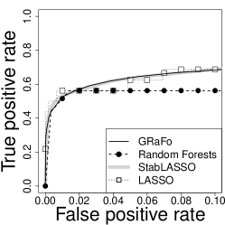
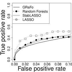
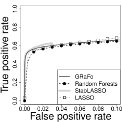
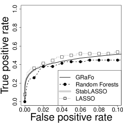
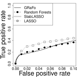
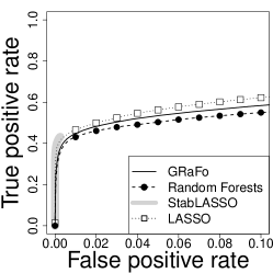
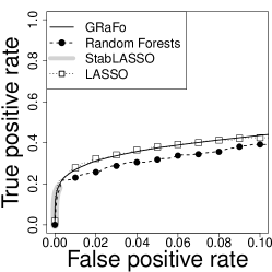
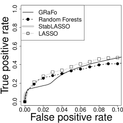
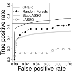
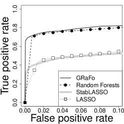
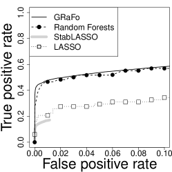
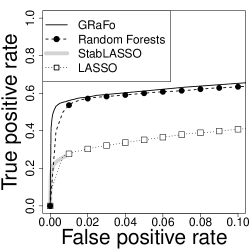
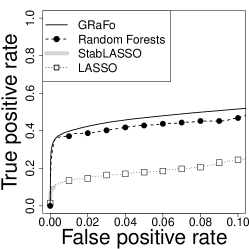
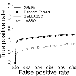
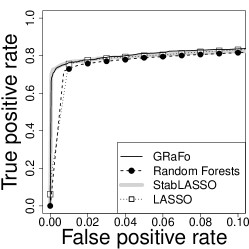
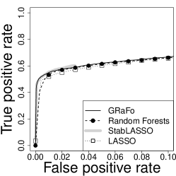
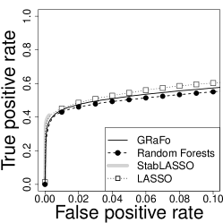
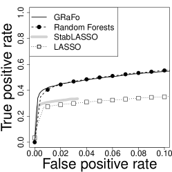
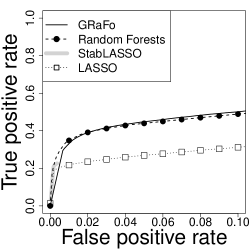
For $p\in\{50,100,200\}$ variables and samples of size $n=100$, each of the $5$ simulation models was averaged over $50$ repetitions. More precisely, for a given $q$, the number of observed true and false positives across the 50 repetitions was averaged. The results are shown in Figures 1-6. Error control for small bounds on the expected number of false positives $\mathbb{E}[V]$ could be achieved for both GRaFo and StabLASSO in all but the mixed setting with $p=200$ in Figure 6.

In the Gaussian, Bernoulli and Ising settings, StabLASSO seems to perform slightly better than GRaFo for small error bounds and rather similar across the figures for the true/false positive rates (third column of Figures 1-3). Note that StabLASSO sets many coefficients to 0. As a consequence, a large proportion of edges cannot be selected for false positive rates smaller than $1$ resulting in some StabLASSO curves not covering the entire range of the rates.

In the multinomial and mixed setting (Figures 4-6), GRaFo returned satisfactory results while StabLASSO performed poorly, presumably caused by dichotomization. In general, both procedures seem to perform best in the Gaussian setting, followed by the mixed, multinomial, Bernoulli, and Ising setting, respectively. The latter seems especially hard for both procedures if the upper error bound in formula (2) for $\mathbb{E}[V]$ is chosen small. Nevertheless, given one’s willingness to expect more errors, the rate figures indicate the potential to recover (parts of) the true structure (cf., Ravikumar et al., 2010; Höfling and Tibshirani, 2009).

The “raw” counterparts, Random Forests and LASSO, correspond to estimations and rankings performed on the full data set without Stability Selection. Consequently, these approaches lack any guidance on choosing $q$. The rate figures were obtained by evaluation of the graphs arising from various values of $q$. We provide them as a means to check if introducing Stability Selection has any additional (positive or negative) effect on the performance of the Random Forests and LASSO methods besides enabling us to choose $q$. From the rate figures, we can deduce that the raw methods perform quite similar to GRaFo and StabLASSO across all settings. Hence, the use of Stability Selection did not introduce any surprising new behavior of Random Forests or LASSO.

A violation of condition (A) of Theorem 1 in the mixed setting could explain the failure of both GRaFo and StabLASSO to achieve error control for $p=200$. However, both the mixed setting with $p=50$ and $p=100$ returned very few observed errors and remained well below the error bounds indicating the problematic behavior may be linked to larger values of $p$. Also, for any setting it is unlikely that the exchangeability assumption holds. Meinshausen and Bühlmann (2010) argue that Stability Selection appears to be robust to violations, but did not study mixed data which may be particularly affected. We study this aspect more closely further below.

The computational cost is growing rather quickly with growing $p$. The runtime of a single of the 50 repetitions per setting is in the order of $15$ minutes for GRaFo and $20$ minutes for StabLASSO for $p=50$ and increases to several hours for GRaFo and $30$ minutes for StabLASSO in the case of $p=200$. Each batch of 50 repetitions was run in parallel on 50 cores of the BRUTUS high-performance cluster comprising quad-core AMD Opteron 8380 2.5 Ghz CPUs with 1 GB of RAM per core using the Rmpi package (Yu, 2010) available in R.

Gaussian, Bernoulli, and Ising models, $p=50$

(a) Gaussian: GRaFo

(b) Gaussian: StabLASSO

(c) Gaussian: Rates

(d) Bernoulli: GRaFo

(e) Bernoulli: StabLASSO

(f) Bernoulli: Rates

(g) Ising: GRaFo

(h) Ising: StabLASSO

(i) Ising: Rates

Figure 1: The rows correspond to the Gaussian, Bernoulli, and Ising model with $p=50$. Their true CIGs have $16$, $16$ and $89$ edges, respectively. The first two columns report the observed number of true and false positives (“o”) relative to the bound in (2) for the expected number $\mathbb{E}[V]$ of false positives (“$]$”) for GRaFo and StabLASSO, respectively, averaged over 50 simulations. The third column reports the averaged true and false positive rates of GRaFo and StabLASSO relative to the performance of their “raw” counterparts without Stability Selection.

Gaussian, Bernoulli, and Ising models, $p=100$

(a) Gaussian: GRaFo

(b) Gaussian: StabLASSO

(c) Gaussian: Rates

(d) Bernoulli: GRaFo

(e) Bernoulli: StabLASSO

(f) Bernoulli: Rates

(g) Ising: GRaFo

(h) Ising: StabLASSO

(i) Ising: Rates

Figure 2: The rows correspond to the Gaussian, Bernoulli, and Ising model with $p=100$. Their true CIGs have $58$, $58$ and $182$ edges, respectively. The first two columns report the observed number of true and false positives (“o”) relative to the bound in (2) for the expected number $\mathbb{E}[V]$ of false positives (“$]$”) for GRaFo and StabLASSO, respectively, averaged over 50 simulations. The third column reports the averaged true and false positive rates of GRaFo and StabLASSO relative to the performance of their “raw” counterparts without Stability Selection.

Gaussian, Bernoulli, and Ising models, $p=200$

(a) Gaussian: GRaFo

(b) Gaussian: StabLASSO

(c) Gaussian: Rates

(d) Bernoulli: GRaFo

(e) Bernoulli: StabLASSO

(f) Bernoulli: Rates

(g) Ising: GRaFo

(h) Ising: StabLASSO

(i) Ising: Rates

Figure 3: The rows correspond to the Gaussian, Bernoulli, and Ising model with $p=200$. Their true CIGs have $334$, $334$ and $369$ edges, respectively. The first two columns report the observed number of true and false positives (“o”) relative to the bound in (2) for the expected number $\mathbb{E}[V]$ of false positives (“$]$”) for GRaFo and StabLASSO, respectively, averaged over 50 simulations. The third column reports the averaged true and false positive rates of GRaFo and StabLASSO relative to the performance of their “raw” counterparts without Stability Selection.

Multinomial and mixed-type models, $p=50$

(a) Multinomial: GRaFo

(b) Multinomial:
(b) StabLASSO (-1/1)

(c) Multinomial: Rates

(d) Mixed: GRaFo

(e) Mixed:
(b) StabLASSO (-1/1)

(f) Mixed: Rates

Figure 4: The rows correspond to the multinomial and mixed-type model with $p=50$. Their true CIGs both have $16$ edges. The first two columns report the observed number of true and false positives (“o”) relative to the bound in (2) for the expected number $\mathbb{E}[V]$ of false positives (“$]$”) for GRaFo and StabLASSO, respectively, averaged over 50 simulations. The third column reports the averaged true and false positive rates of GRaFo and StabLASSO relative to the performance of their “raw” counterparts without Stability Selection.

Multinomial and mixed-type models, $p=100$

(a) Multinomial: GRaFo

(b) Multinomial:
(b) StabLASSO (-1/1)

(c) Multinomial: Rates

(d) Mixed: GRaFo

(e) Mixed:
(b) StabLASSO (-1/1)

(f) Mixed: Rates

Figure 5: The rows correspond to the multinomial and mixed-type model with $p=100$. Their true CIGs both have $58$ edges. The first two columns report the observed number of true and false positives (“o”) relative to the bound in (2) for the expected number $\mathbb{E}[V]$ of false positives (“$]$”) for GRaFo and StabLASSO, respectively, averaged over 50 simulations. The third column reports the averaged true and false positive rates of GRaFo and StabLASSO relative to the performance of their “raw” counterparts without Stability Selection.

Multinomial and mixed-type models, $p=200$

(a) Multinomial: GRaFo

(b) Multinomial:
(b) StabLASSO (-1/1)

(c) Multinomial: Rates

(d) Mixed: GRaFo

(e) Mixed:
(b) StabLASSO (-1/1)

(f) Multinomial: Rates

Figure 6: The rows correspond to the multinomial and mixed-type model with $p=200$. Their true CIGs both have $334$ edges. The first two columns report the observed number of true and false positives (“o”) relative to the bound in (2) for the expected number $\mathbb{E}[V]$ of false positives (“$]$”) for GRaFo and StabLASSO, respectively, averaged over 50 simulations. The third column reports the averaged true and false positive rates of GRaFo and StabLASSO relative to the performance of their “raw” counterparts without Stability Selection.

4.4 Simulation Results: Gaussian with Interaction Effects

For $p\in\{50,100,200\}$ variables and samples of size $n=100$, each graph in Figure 7 was averaged over $50$ repetitions. The results appear very similar to our findings for the Gaussian model without interactions and without nonlinear effects. However, here the number of true positives is somewhat lower for both GRaFo and StabLASSO with an (arguably) slightly smaller drop for the GRaFo procedure. This does not seem too surprising, given that Random Forests have the ability to incorporate interactions naturally, whereas they have to be specified explicitly for the LASSO (which has not been done here).

However, overall the total number of interaction terms is relatively small, ranging from roughly 5% to 10% of all model terms. For a larger number of interaction terms, we would thus expect a further gain of the GRaFo over the StabLASSO procedure.

Gaussian with interaction effects $p=50$, $100$, and $200$

(a) Interaction, $p=50$:
(a) GRaFo

(b) Interaction, $p=50$:
(b) StabLASSO

(c) Interaction, $p=50$:
(c) Rates

(d) Interaction, $p=100$:
(d) GRaFo

(e) Interaction, $p=100$:
(e) StabLASSO

(f) Interaction, $p=100$:
(e) Rates

(g) Interaction, $p=200$:
(f) GRaFo

(h) Interaction, $p=200$:
(h) StabLASSO

(i) Interaction, $p=200$:
(i) Rates

Figure 7: Gaussian model with interactions with $p=50$, $100$, and $200$. Their true CIGs have $16$, $58$, and $334$ edges, respectively, with $1$, $6$, and $21$ first-order interaction terms. The first two columns report the observed number of true and false positives (“o”) relative to the bound in (2) for the expected number $\mathbb{E}[V]$ of false positives (“$]$”), respectively, averaged over 50 simulations. The third column reports the averaged true and false positive rates of GRaFo and StabLASSO relative to the performance of their “raw” counterparts without Stability Selection.

4.5 Simulation Results: Gaussian with Nonlinear Effects

For $p\in\{50,100,200\}$ variables and samples of size $n=100$, each graph in Figure 8 was averaged over $50$ repetitions. Here, GRaFo clearly outperforms StabLASSO in terms of true positives for all considered $p$. However, for GRaFo the number of false positives is not controlled by a small bound on $\mathbb{E}[V]$ anymore for $p>50$, which is especially apparent in the case where $p=200$. For StabLASSO there seems to be a similar behavior, but only for $p=200$ the number of false positives clearly violates $\mathbb{E}[V]$. The “raw” Random Forests and LASSO estimates show very similar results to their Stability Selection counterparts. Note that the signal has been amplified by a factor of 5 to achieve comparable performance of the estimation procedures to the linear Gaussian setting.

Gaussian with nonlinear effects $p=50$, $100$, and $200$

(a) Nonlinear, $p=50$:
(a) GRaFo

(b) Nonlinear, $p=50$:
(b) StabLASSO

(c) Nonlinear, $p=50$:
(c) Rates

(d) Nonlinear, $p=100$:
(d) GRaFo

(e) Nonlinear, $p=100$:
(e) StabLASSO

(f) Nonlinear, $p=100$:
(f) Rates

(g) Nonlinear, $p=200$:
(g) GRaFo

(h) Nonlinear, $p=200$:
(h) StabLASSO

(i) Nonlinear, $p=200$:
(i) Rates

Figure 8: The rows correspond to the Gaussian with nonlinear associations with $p=50$, $100$, and $200$. Their true CIGs have $16$, $58$, and $334$ edges, respectively. The first two columns report the observed number of true and false positives (“o”) relative to the bound in (2) for the expected number $\mathbb{E}[V]$ of false positives (“$]$”) for GRaFo and StabLASSO, respectively, averaged over 50 simulations. The third column reports the averaged true and false positive rates of GRaFo and StabLASSO relative to the performance of their “raw” counterparts without Stability Selection.

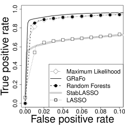
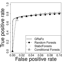
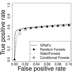
4.6 Simulation Results: Mixed-Setting with ML and StabCForests

The first row of Figure 9 reports for $p=50$ and $n=500$ the results of ML estimation, GRaFo, and StabLASSO, averaged over 50 runs. Not surprising, both GRaFo and StabLASSO perform better than in the setting where $n=100$, though StabLASSO remains at a clear disadvantage due to the unfavorable dichotomization. On the other hand, the performance of GRaFo (and also its “raw” Random Forests counterpart) is on par with the ML estimation. Stability Selection was not applied to ML estimation due to the immense computational burden and thus no bounds on $\mathbb{E}[V]$ could be specified. However, for both GRaFo and StabLASSO we find that the number of false positives are typically well below the specified bounds.

The second and third row of Figure 9 report the performance of StabcForests and GRaFo for $p=50$ and $p=100$ with $n=100$, averaged over 50 runs. The GRaFo results from above are reproduced for better readability. We find that both GRaFo and StabcForests show very similar results. In the first two columns we see that GRaFo seems to perform somewhat better for very small bounds on $\mathbb{E}[V]$. The performance of the two “raw” methods is very similar to their stable counterparts.

The computational burden of StabcForests is much larger than for GRaFo and amounts to roughly 2 hours for $p=50$ and roughly 6 hours for $p=100$. Also note that the reported results within the Conditional Forests framework use the marginal permutation importance due to the very heavy computational burden of the conditional variable importance.

Mixed setting with ML and StabcForests with $p=50$, $100$, and $200$

(a) Mixed, $p=50$, $n=500$:
(a) GRaFo

(b) Mixed, $p=50$, $n=500$:
(b) StabLASSO

(c) Mixed, $p=50$, $n=500$:
(c) Rates

(d) Mixed, $p=50$, $n=100$:
(d) GRaFo

(e) Mixed, $p=50$, $n=100$:
(e) StabcForests

(f) Mixed, $p=50$, $n=100$:
(f) Rates

(g) Mix., $p=100$, $n=100$:
(g) GRaFo

(h) Mix., $p=100$, $n=100$:
(h) StabcForests

(i) Mix., $p=100$, $n=100$:
(i) Rates

Figure 9: The rows correspond to applications of ML and StabcForests to data from the mixed model with varying $p$ and $n$. For $p=50$ ($p=100$), the true CIG has $16$ ($58$) edges. The first two columns report the observed number of true and false positives (“o”) relative to the bound in (2) for the expected number $\mathbb{E}[V]$ of false positives (“$]$”) for GRaFo and StabLASSO or StabcForests, respectively, averaged over 50 simulations. The third column reports the averaged true and false positive rates.

5 Functional Health in the Swiss General Population

5.1 The Importance of Functional Health

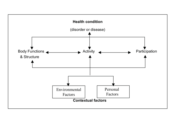
According to the World Health Organization’s (WHO) new framework of the International Classification of Functioning, Disability and Health (ICF; cf., WHO, 2001) the lived experience of health (Stucki et al., 2008) can be structured in experiences related to body functions and structures as well as to activity and participation in society. All of these are, in turn, influenced by a variety of so-called personal factors such as gender, income, or age and environmental factors including individual social relations and supports as well as properties of larger macro social systems such as the economy (see Figure 10). Also, the WHO and The World Bank recommend in their recent World Report on Disability (2011) that functional health state descriptors are analyzed in conjunction with other health outcomes and, particularly, that more research is conducted on “[…] the interactions among environmental factors, health conditions, and disability […]” (p. 267 WHO and The World Bank, 2011). Under these prerequisites it is of interest which variables are conditionally dependent on each other. For instance, “Does the income distribution affect participation, conditional on known impairments, environmental, and personal factors?”.

Figure 10: The International Classification of Functioning, Disability and Health (ICF) model relates aspects of human functioning and provides a common language for practitioners.

5.2 Study Population

We use GRaFo for a secondary analysis of cross-sectional observational data on functional health from the Swiss Health Survey (SHS) in 2007. Data were obtained from the Federal Statistics Office of Switzerland. The original study was based on a stratified random sample of all private Swiss households with fixed line telephones. Within each household one household member aged 15 or older was randomly selected. The survey was completed by a total of 18760 persons, corresponding to a participation rate of 66 percent (Graf, 2010). The mean age of study participants was 49.6 years $(\pm 18.5)$. The data were mostly collected with computer assisted telephone interviews. Further information is available elsewhere (Storni, 2011).

5.3 Variables

The SHS included various information on symptoms (in particular pain), impairments, and activity limitations. Since the respective items were sometimes nominal, sometimes ordinal, and sometimes (e.g. body mass index) metric, we dichotomized each item so that 1 was indicative of having any kind of problem. As overall summary scores on functioning and disability were not recommendable (Reinhardt et al., 2010), we followed the framework of the WHO’s biopsychosocial model of health, outlined in the ICF (WHO, 2001, see Figure 10), and other theoretical considerations (WHO and The World Bank, 2011; Reinhardt et al., 2010) in constructing sum indices (see Table 2). The plausibility of all indices was checked using the Stata 11 confirmatory factor analysis module confa (Kolenikov, 2009). In each case the index construction was tested and the null hypothesis of a diagonal structure of the covariance matrix rejected.

We created a dummy variable for labor market participation restrictions such that 1 identified persons who gave up work, reduced the number of working hours, or changed jobs because of health reasons. We also created a dummy variable for participation in leisure physical activity (LPA) differentiating between people participating in leisure activities leading to sweating at least once a week and those who do not. General health perception was measured with the following question and answer options: “How would you rate your health in general? Very good, good, fair, poor, or very poor?”. We further included indicators of socio-economic status (SES) in our analysis: equivalence household income, years of formal education, employment status, and migration background (foreign origin of at least one parent). On the macro- or cantonal-level we obtained information on the Swiss counties’ (cantons) gross domestic products (GDP), Gini coefficients, and crime rates for 2006. Moreover, we considered information on gender, age, marital status (being married), alcohol consumption (in grams per day), and current smoking (yes/no).

Of these, in total, 20 mixed-type variables (see Table 3), income had the highest number of missing values with roughly 6 percent. Overall, less than 0.85 percent of replies were missing corresponding to 2687 cases with one or more missing values. To assess their effect, we estimated the CIG once with casewise deletion and once with imputation of missing values with the missForest procedure (Stekhoven and Bühlmann, 2011) available in R. An alternative would be to use surrogate splits, which may be particularly feasible if the speed of the imputation method is of importance (Hapfelmeier et al., 2012).

Construct	Variable specification
Impairment	Problems with$\ldots$
	$\ldots$vision
	$\ldots$hearing
	$\ldots$speaking
	$\ldots$body mass index (i.e. over 30 or under 16)
	$\ldots$urinary incontinence
	$\ldots$defecation
	$\ldots$feeling weak, tired, or a lack of energy
	$\ldots$sleeping
	$\ldots$tachycardia
	Range of sum index: 0-9
Pain	Pain in$\ldots$
	$\ldots$head
	$\ldots$chest
	$\ldots$stomach
	$\ldots$back
	$\ldots$hands
	$\ldots$joints
	Range of sum index: 0-6
Activity &	Problems with independently$\ldots$
participation	$\ldots$walking
limitation	$\ldots$eating
	$\ldots$getting up from bed or chair
	$\ldots$dressing
	$\ldots$using the toilet
	$\ldots$taking a shower or bath
	$\ldots$preparing meals
	$\ldots$using a telephone
	$\ldots$doing the laundry
	$\ldots$caring for finances/accounting
	$\ldots$using public transport
	$\ldots$doing major household tasks
	$\ldots$doing shopping
	Range of sum index: 0-13
Social support	Having$\ldots$
	$\ldots$no feelings of loneliness
	$\ldots$no desire to turn to someone
	$\ldots$at least one supportive family member
	$\ldots$someone to turn to
	Range of sum index: 0-4
Social network utilization	At least weekly$\ldots$
	$\ldots$visits from family
	$\ldots$phone calls with family
	$\ldots$visits from friends
	$\ldots$phone calls with friends
	$\ldots$participation in clubs/associations/parties
	Range of sum index: 0-5

Table 2: Construction rules of sum indices for functioning (pain, impairment, activity and participation limitation) and social integration (social support and social network utilization) from 37 dichotomous (yes=1/no=0) variables.

Type	Variable	% Missing
$>2$ categories	Impairment index	5.92
	Pain index	0.37
	Activity limitation index	0.69
	Social support index	5.84
	Social network utilization index	2.32
	General health perception	0.05
Dichotomous	Male	0.00
	Married	0.09
	Paid work	0.03
	Migration background	4.73
	Smoker	0.07
	Work restriction	0.00
	Leisure physical activity	0.00
Continuous	Age	0.00
	Years of formal education	0.07
	Income	5.94
	Alcohol consumption (in grams per day)	2.59
	Gross domestic product	0.00
	Gini coefficient	0.00
	Crime rate	0.00

Table 3: List of all 20 variables used in the CIG estimation, their type, and their percentage of missing values.

5.4 Research Hypothesis

From the WHO’s ICF model (WHO, 2001, see Figure 10), we hypothesized that all variables on functional and general health perception, and all variables on social status, networks, and supports were connected via paths within the same component of the CIG.

5.5 Findings

Figure 11: Conditional independence graph of the $p=20$ variables (nodes) remaining after construction of indices based on the 2007 Swiss Health Survey estimated with GRaFo. Edges were selected with respect to an upper bound of 5 on the expected number of false positives, see formula (2). Five nodes (social network utilization, migration background, smoker, work restriction, and LPA) were isolated (no edges) and thus neglected.

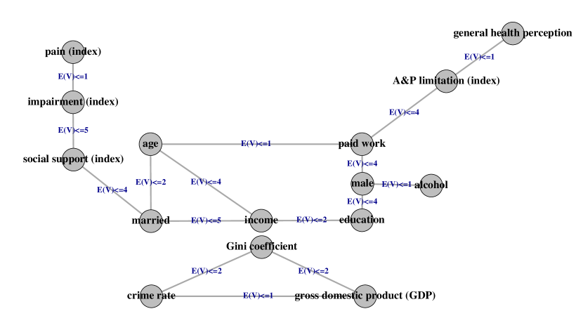
Figure 11 shows the resulting graph from our application of GRaFo to the (non-imputed) data on functional health from the SHS with casewise deletion of missing values regularized for a bound (as in formula (2)) for an expected number of false positives $\mathbb{E}[V]\leq 5$. The selected edge sets for the imputed and casewise deleted data were quite similar for various bounds on $\mathbb{E}[V]$ and even identical for $\mathbb{E}[V]\leq 5$ (not shown). In the following, we thus focus on the CIG derived from the complete observations remaining after casewise deletion of missing values. As the data contains mixed-type variables we did not perform a similar analysis with the LASSO (clearly non-favorable dichotomization was used in the simulations in Section 4.3).

The resulting edges for $\mathbb{E}[V]\leq 1$ depict relatively obvious associations known from everyday observations. Interestingly, general health perception is conditionally dependent on activity limitation but conditionally independent of impairment and pain. In the larger graph for $\mathbb{E}[V]\leq 5$, one sees that general health perception, impairments, and pain are connected through a path of several environmental and personal factors such as social support, being married, age, etc. That implies, for instance, that we do not need information on impairment to predict general health perception if we have information on activity limitation and the remaining predictors, whereas activity limitation is an essential predictor of general health perception even if information on all the remaining predictors is provided. For instance, a person with a spinal cord injury who has no activity limitation because of social and technological supports, could thus still report good health. This finding is supported by other sources reporting that many people with disabilities do not consider themselves to be unhealthy (WHO and The World Bank, 2011; Watson, 2002). In the 2007-2008 Australian National Health Survey, 40 percent of people with a severe or profound impairment rated their health as good, very good, or excellent (Australian Bureau of Statistics, 2009).

As regards our hypothesis derived from the ICF model (WHO, 2001), we can confirm that the bulk of individual level variables form one component and support the biopsychosocial model of health: Functional and general health influence each other and are connected with a variety of environmental and personal factors. However, not all candidate personal and environmental factors were related in our study. This may be due to our conservative upper bound on the error that is likely to favor false negatives, i.e. missing edges. There may also be an issue with our selection of variables that was restricted by the choices of the original survey team. In particular, macro-level variables pertaining information about the counties, in which the individuals are nested, form a second component. It may be that their effect is already contained in the individual-level variables, for example paid work. Five variables do not appear in the graph entirely: social network utilization, migration background, smoker, work restriction, and LPA. If we remove the three macro-level variables GDP, Gini, and crime rate from the model, the connectivity of the individual-level component does not change. Instead, the two variables migration background and social network utilization are now present as a separate component (not shown).

Unfortunately, lack of information on the directions of relationships is a weakness of CIGs. Also, condition (A) of Theorem 1 and the exchangeability condition have likely been violated. One disadvantage of the randomForest implementation is the inability to model continuous variables with $<6$ unique values, which may oftentimes be an issue for the sum indices in combination with subsampling. Consequently, we chose to model them as categorical variables. Regardless, given the high face validity of the findings and the achievement of error control in the mixed setting for small $p$ in Section 4.3, the results seem satisfactory.

The runtime of GRaFo depends also on $n$, even if $p$ is small. Hence, estimation of the SHS graph was executed in parallel on 10 cores of the BRUTUS cluster with a runtime of roughly 8 hours.

6 Modeling Neurodevelopment in Children Experiencing Open-Heart Surgery

Here we demonstrate an application of GRaFo to a research question, where $p$ is much larger than $n$. It is thus of particular interest, whether GRaFo can suggest meaningful associations or tends to produce seemingly spurious associations.

6.1 Neurodevelopment after Open-Heart Surgery

In children with complex congenital heart disease (CHD) neurological and developmental alterations are common (Bellinger et al., 2003; Snookes et al., 2010; Ballweg et al., 2007). The observed cognitive, behavioral, and motor deficits can significantly impact daily routine and educational perspectives and lead to a high rate of special schooling and supportive therapies in this population (von Rhein et al., ; Hövels-Gürich et al., 2006, 2008). In severe congenital heart disease requiring open-heart surgery, factors can be further subdivided into pre-, peri-, and post-operative factors. One of the major limitations of studies on patient specific risk-factors (Ballweg et al., 2007; Hövels-Gürich et al., 2006, 2008), treatment and bypass protocols (Bellinger et al., 2003; Snookes et al., 2010), and post-operative complications (Bellinger et al., 2003; Snookes et al., 2010) is the inability to provide a full picture of the interplay of all potentially relevant risk-factors available in the data. Thus, understanding their common association structure is of large interest.

6.2 Study Population

A group of 221 infants with a congenital heart disease that underwent open-heart surgery with full-flow cardiopulmonary bypass prior to their first birthday from a study of the Children Hospital Zurich from 2004 to 2008 (von Rhein et al., ). We restricted our sample to a more homogeneous sub-population of 34 infants suffering from trisomy 21 of whom 14 were male and 31 caucasian.

6.3 Variables

In total, 133 variables were available for modeling. They can further be subdivided into 40 variables describing basic characteristics (e.g. birth parameters, family information), 10 variables characterizing a child’s neurodevelopment prior to surgery, 69 peri-operative factors (i.e. data on pre-operative, intra-operative, and post-operative course), 13 variables characterizing a child’s neurodevelopment 1 year post surgery, and 1 variable summarizing quality of life based on the TAPQOL questionnaire (TNO, 2004).

To ease interpretation, we focus in Table 4 on the 29 variables which had at least one adjacent node in the resulting graph which we discuss below. These variables are of mixed-type, with 23 continuous variables and 6 factors with more than 2 levels.

Outcome-variables of primary interest are the Bayley score for motor development and the Bayley score for cognitive development (Bayley, 1993). Both scores were assessed at one year of age.

Scale	Group	Variable	Missing
cont	birth/family	Apgar score 5 mins	11
cont	birth/family	Apgar score 1 mins	11
cont	birth/family	Apgar score 10 mins	10
cont	birth/family	birth weight	1
cont	birth/family	gestational age	0
cont	birth/family	birth length	1
cont	birth/family	father age	1
cont	birth/family	mother age	0
$>2$	birth/family	father school education	2
$>2$	birth/family	father professional education	2
cont	birth/family	socio economic status	1
$>2$	birth/family	mother school education	1
$>2$	birth/family	mother number pregnancies	1
$>2$	birth/family	mother number births gestational age $>24$ weeks	1
cont	peri-operative	time aorta occlusion	0
$>2$	peri-operative	operation risk	0
cont	peri-operative	lactate max during surgery	1
cont	peri-operative	lactate max 24h post surgery	0
cont	peri-operative	age at surgery	0
cont	peri-operative	lowest SO2 during surgery	0
cont	peri-operative	lowest SO2 24h post surgery	0
cont	peri-operative	length at surgery	0
cont	peri-operative	weight at surgery	0
cont	peri-operative	head circumference at surgery	0
cont	1 year post surgery	weight at 1 year	5
cont	1 year post surgery	length at 1 year	5
cont	1 year post surgery	head circumference at 1 year	5
cont	1 year post surgery	Bayley motor score	5
cont	1 year post surgery	Bayley cognitive score	6

Table 4: List of all 29 variables which appear in the graph, their scale type ($>2$ for categorical; cont. for continuous) , variable group, and their percentage of missing values.

In total, 3.4 percent of the data were missing, ranging from 87 completely observed variables to 3 variables with 11 missing observations (two Apgar score variables (see also Apgar, 1953) and the child’s head circumference at birth (not in graph)). Case-wise exclusion of children with missing values seems infeasible as this would result in the loss of 26 children. Data were thus imputed using the missForest procedure (Stekhoven and Bühlmann, 2011).

6.4 Objective

To identify risk-factors associated with the cognitive and motor development of infants that have undergone open-heart surgery in the first 12 months after birth due to a congenital heart disease using GRaFo.

Due to the large number of variables, many methods of analysis (such as bivariate correlations) may be prone to yield various spurious associations. It is here thus also of interest to demonstrate that, whenever GRaFo suggests an association, it tends to have a high face validity (which is judged by the collaborating health professionals).

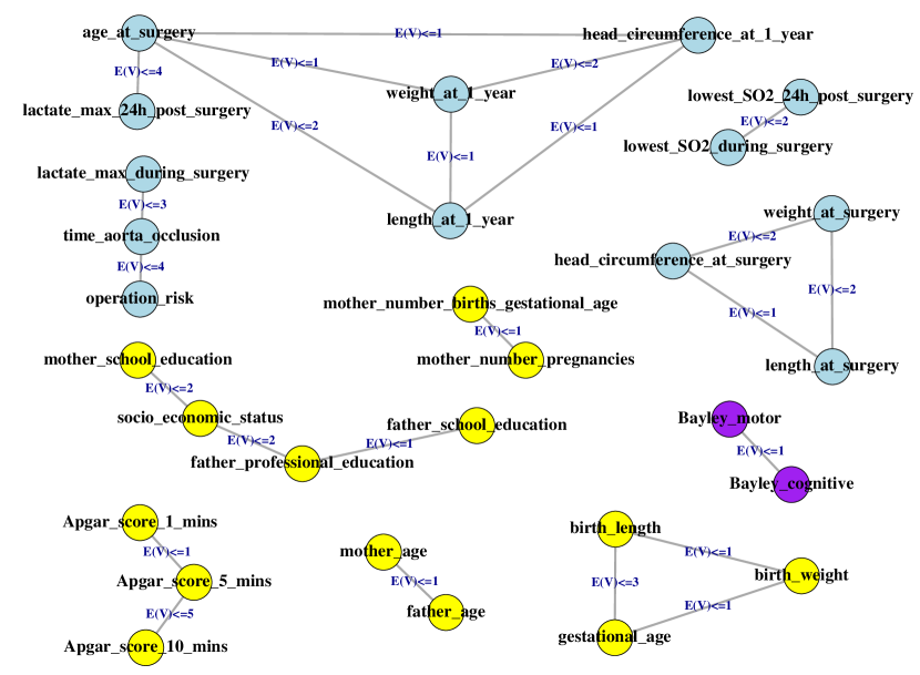
6.5 Findings

For an upper bound of 5 on the expected number of false positives $\mathbb{E}[V]$ we find that the Balyey scores for motor and cognitive development are only associated with each other, but not with any other node in the graph (conditional the remainder) in Figure 12. We do, however, find 10 small clusters of high face-validity. For example, the age of each child’s father and mother form a common cluster. Likewise, the children’s Apgar score after 1 minute is connected with the Apgar score after 5 minutes. The latter furthermore connects with the Apgar score after 10 minutes. It thus seems that GRaFo manages to identify many edges which appear intuitively correct, but it fails to provide new insights into the association structure of the Bayley scores. On the other hand, no apparent “odd” associatons were suggested.

This result mirrors current knowledge about the neurodevelopment of infants after open heart surgery: genetic defects (Bellinger et al., 2003; Snookes et al., 2010; Ballweg et al., 2007) and ethnicity (Ballweg et al., 2007) have been described as relevant risk-factors for adverse neurodevelopment. As we mostly worked with caucasian children, all of whom have trisomy 21, these factors have already been controlled for by the design. Even if we increase the upper bound on $\mathbb{E}[V]$ to 50 we still cannot find any additional variables connected to the Bayley scores. The plausibility of the other observed clusters would thus suggest, that no stable associations with the Bayley scores can be identified using GRaFo.

Figure 12: The figure shows the conditional independence graph of children with trisomy 21 experiencing open-heart surgery. The reported $p=29$ variables (nodes) have at least one adjacent node for an upper bound of 5 on the expected number of false positives $\mathbb{E}[V]$.

However, potential bias induced by the imputation method which also utilizes Random Forests cannot be excluded. For example, all Apgar scores showed a large number of missing values. The identified cluster may thus also be an artifact of the missing value imputation. Furthermore, our choice of variables was determined by the original study design. Also, we cannot guarantee that the exchangeability assumption (Meinshausen and Bühlmann, 2010) and assumption (A) from Theorem 1 hold.

The small number of children ($n\ll p$) allowed to run this analysis on an AMD Athlon 64 X2 5600+ PC with 6 GB of memory in just under 14 minutes.

7 Conclusion

We propose GRaFo (Graphical Random Forests) performed satisfactory, mostly on par or superior to StabLASSO, StabcForests, LASSO, Conditional Forests, Random Forests, and ML estimation. Error control of false positive edges could be achieved in all but the mixed-type simulation with $p=200$ and the nonlinear Gaussian setting with $p\geq 100$. Violation of assumption (A) in Theorem 1 and of the exchangeability condition might be responsible for this behavior. In contrast, in most of the other settings GRaFo was very conservative and observed false positive edges were well below their expected upper bound. The Ising model, the sole model not based on DAGs, was particularly hard for both GRaFo and StabLASSO resulting in few true positives if error bounds were chosen very small.

Results in the Gaussian setting with interactions were very similar to the main effects Gaussian setting, which is likely due to the small number of interactions in our simulation model. On the contrary, GRaFo shows a clear gain over StabLASSO in the nonlinear setting, where half of the associations were nonlinear in nature.

Poor results for the LASSO in the multinomial and mixed case, where we need dichotomization, may be improved by feasible modifications of the LASSO, such as an extension of the group LASSO (Meier et al., 2008) to multinomial responses (Dahinden et al., 2010). However, penalization if both discrete and continuous variables are included is not a straightforward task (including the issue of scaling).

The ML results indicate that both GRaFo and StabcForests perform very well in the mixed setting, though the computational cost of StabcForests notably exceeds the cost of GRaFo. Both Forests-based algorithms used marginal permutation importance as the conditional permutation importance turned out impractical due to its high computational cost.

The Swiss Health Survey graph consists of an individual- and a macro-level variable cluster which were highly stable with respect to the way of handling missing values. Exclusion of the macro-level cluster did not affect the individual-level cluster. For a small error bound, our hypothesis that all factors should connect could not be fully confirmed, though a strong tendency toward the ICF’s biopsychosocial model of health was evident in the individual-level cluster.

The children hospital graph consists of many clusters of high face-validity. We believe this emphasizes GRaFo’s potential to isolate true and stable associations. However, we failed to identify any new potential risk factors that may help to explain adverse neurodevelopment (since no edges connect to the corresponding outcome measures). The known risk factors ethnicity and genetic defects were controlled for by the design. This may be a consequence of the available pool of variables. Also, it is imaginable, that some associations are only of importance for a sub-group of the study. In this case, they would appear to be instable to GRaFo and consequently not be reported.

8 Proof of Theorem 1

Proof: We know that $X_{j}\mathchoice{\mathrel{\hbox to0.0pt{$\displaystyle\perp$\hss}\mkern 2.0mu{\displaystyle\perp}}}{\mathrel{\hbox to0.0pt{$\textstyle\perp$\hss}\mkern 2.0mu{\textstyle\perp}}}{\mathrel{\hbox to0.0pt{$\scriptstyle\perp$\hss}\mkern 2.0mu{\scriptstyle\perp}}}{\mathrel{\hbox to0.0pt{$\scriptscriptstyle\perp$\hss}\mkern 2.0mu{\scriptscriptstyle\perp}}}X_{i}|{\bf X}\setminus\{X_{j},X_{i}\}$ is equivalent to

$$\mathbb{P}[X_{j}\leq x_{j}|\{x_{h};h\neq j\}]=\mathbb{P}[X_{j}\leq x_{j}|\{x_{h};h\neq j,i\}]$$ (4)

for all realizations $x_{j}$ of $X_{j}$ and $\{x_{h};h\neq j\}$ of ${\bf X}\setminus\{X_{j}\}$. Due to assumption (A) we can rewrite (4):

$$F_{j}(x_{j}|m_{j}(\{x_{h};h\neq j\}))=F_{j}(x_{j}|m_{j}(\{x_{h};h\neq j,i\}))$$ (5)

for all $x_{j}$ and all $\{x_{h};h\neq j\}$. But (5) is equivalent to

$$m_{j}(\{x_{h};h\neq j\})=m_{j}(\{x_{h};h\neq j,i\})$$ (6)

for all $\{x_{h};h\neq j\}$. This completes the proof.

9 Acknowledgment

The authors would like to thank three anonymous reviewers, Gerold Stucki, Markus Kalisch, Marloes Maathuis, Philipp Rütimann, and Holger Höfling for valuable feedback and discussion.

10 References

References

- Altman and Royston (2006) Altman, D.G., Royston, P., 2006. The cost of dichotomising continuous variables. Brit Med J 332, 1080.
- Amit and Geman (1997) Amit, Y., Geman, D., 1997. Shape quantization and recognition with randomized trees. Neural Comput 9, 1545–1588.
- Apgar (1953) Apgar, V., 1953. A proposal for a new method of evaluation of the newborn infant . in: 32 (1953),. Curr. Res. Anesth. Analg. 32, 260 –267.
- Archer (2010) Archer, K.J., 2010. rpartOrdinal: An R package for deriving a classification tree for predicting an ordinal response. J Stat Softw 34, 1–17.
- Australian Bureau of Statistics (2009) Australian Bureau of Statistics, 2009. National Health Survey: Summary of Results, 2007-2008. Australian Bureau of Statistics, Canberra.
- Ballweg et al. (2007) Ballweg, J.A., Wernovsky, G., Gaynor, J.W., 2007. Neurodevelopmental outcomes following congenital heart surgery. Pediatr Cardiol 28, 126–33.
- Bayley (1993) Bayley, N., 1993. Manual for the Bayley Scales of Infant Development. The Psychological Corporation, San Antonio, TX.
- Bellinger et al. (2003) Bellinger, D.C., Wypij, D., duPlessis, A.J., Rappaport, L.A., Jonas, R.A., Wernovsky, G., Newburger, J.W., 2003. Neurodevelopmental status at eight years in children with dextro-transposition of the great arteries: the Boston Circulatory Arrest Trial. J Thorac Cardiov Sur 126, 1385–96.
- Breiman (1996) Breiman, L., 1996. Bagging predictors. Mach Learn 24, 123–140.
- Breiman (2001) Breiman, L., 2001. Random Forests. Mach Learn 45, 5–32.
- Breiman (2002) Breiman, L., 2002. Setting Up, Using, And Understanding Random Forests V4.0.
- Breiman et al. (1984) Breiman, L., Friedman, J., Olshen, R., Stone, C., 1984. Classification and Regression Trees. Wadsworth, Inc., California.
- Bühlmann and Yu (2002) Bühlmann, P., Yu, B., 2002. Analyzing bagging. Ann Stat 30, 927–961.
- Dahinden et al. (2010) Dahinden, C., Kalisch, M., Bühlmann, P., 2010. Decomposition and model selection for large contingency tables. Biometrical J 7, 247–248.
- Efron (1979) Efron, B., 1979. Bootstrap methods: Another look at the jackknife. Ann Stat 7, 1–26.
- Friedman et al. (2008) Friedman, J., Hastie, T., Tibshirani, R., 2008. Sparse inverse covariance estimation with the graphical Lasso. Biostatistics 9, 432–441.
- Friedman et al. (2010) Friedman, J., Hastie, T., Tibshirani, R., 2010. Regularization paths for generalized linear models via coordinate descent. J Stat Softw 33, 1–22.
- Givens and Hoeting (2005) Givens, G.H., Hoeting, J.A., 2005. Computational Statistics. Hohn Wiley & Sons, Inc., New Jersey.
- Graf (2010) Graf, E., 2010. Rapport de méthodes. Enquête suisse sur la santé 2007. Plan d’échantillonnage, pondérations et analyses pondérées des données. Office Fédéral de la Statistique, Neuchâtel.
- Hapfelmeier et al. (2012) Hapfelmeier, A., Hothorn, T., Ulm, K., 2012. Recursive partitioning on incomplete data using surrogate decisions and multiple imputation. Comput Stat Data An 56, 1552–1565.
- Höfling and Tibshirani (2009) Höfling, H., Tibshirani, R., 2009. Estimation of sparse binary pairwise markov networks using pseudo-likelihoods. J Mach Learn Res 10, 883–906.
- Hothorn et al. (2006) Hothorn, T., Hornik, K., Zeileis, A., 2006. Unbiased recursive partitioning: A conditional inference framework. Journal of Computational and Graphical Statistics 15, 651–674.
- Hövels-Gürich et al. (2008) Hövels-Gürich, H.H., Bauer, S.B., Schnitker, R., Willmes-von Hinckeldey, K., Messmer, B.J., Seghaye, M.C., Huber, W., 2008. Long-term outcome of speech and language in children after corrective surgery for cyanotic or acyanotic cardiac defects in infancy. Eur J Paediatr Neuro 12, 378–86.
- Hövels-Gürich et al. (2006) Hövels-Gürich, H.H., Konrad, K., Skorzenski, D., Nacken, C., Minkenberg, R., Messmer, B.J., Seghaye, M.C., 2006. Long-term neurodevelopmental outcome and exercise capacity after corrective surgery for tetralogy of Fallot or ventricular septal defect in infancy. Ann Thorac Surg 81, 958–66.
- Kalisch and Bühlmann (2007) Kalisch, M., Bühlmann, P., 2007. Estimating high-dimensional directed acyclic graphs with the PC-algorithm. J Mach Learn Res 8, 613–636.
- Kalisch et al. (2010) Kalisch, M., Fellinghauer, B., Grill, E., Maathuis, M.H., Mansmann, U., Bühlmann, P., Stucki, G., 2010. Understanding human functioning using graphical models. BMC Med Res Methodol 10, 14.
- Kolenikov (2009) Kolenikov, S., 2009. Confirmatory factor analysis using confa. Stata J 9, 329–373.
- Lauritzen (1996) Lauritzen, S.L., 1996. Graphical Models. Oxford University Press, Oxford.
- Lauritzen and Spiegelhalter (1988) Lauritzen, S.L., Spiegelhalter, D.J., 1988. Local computations with probabilities on graphical structures and their application to expert systems (with discussion). J Roy Stat Soc B 50, 157–224.
- Lauritzen and Wermuth (1989) Lauritzen, S.L., Wermuth, N., 1989. Graphical models for associations between variables, some of which are qualitative and some quantitative. Ann Stat 17, 31–57.
- Liaw and Wiener (2002) Liaw, A., Wiener, M., 2002. Classification and regression by randomForest. R News 2, 18–22.
- Lokhorst (1999) Lokhorst, J., 1999. The Lasso and generalised linear models. Honors project. The University of Adelaide, Australia.
- MacCallum et al. (2002) MacCallum, R.C., Zhang, S., Preacher, K.J., Rucker, D.D., 2002. On the practice of dichotomization of quantitative variables. Psychol Methods 7, 19–40.
- Meier et al. (2008) Meier, L., van de Geer, S., Bühlmann, P., 2008. The group Lasso for logistic regression. J Roy Stat Soc B 70, 53–71.
- Meinshausen and Bühlmann (2006) Meinshausen, N., Bühlmann, P., 2006. High-dimensional graphs and variable selection with the Lasso. Ann Stat 34, 1436–1462.
- Meinshausen and Bühlmann (2010) Meinshausen, N., Bühlmann, P., 2010. Stability selection (with discussion). J Roy Stat Soc B 72, 417–473.
- Nicodemus et al. (2010) Nicodemus, K.N., Malley, J.D., Strobl, C., Ziegler, A., 2010. The bahaviour of Random Forest permutation-based variable importance measures under predictor correlation. BMC Bioinformatics 11.
- Politis et al. (1999) Politis, D.N., Romano, J.P., Wolf, M., 1999. Subsampling. Springer, Berlin.
- R Development Core Team (2011) R Development Core Team, 2011. R: A Language and Environment for Statistical Computing. R Foundation for Statistical Computing. Vienna, Austria. ISBN 3-900051-07-0.
- Ravikumar et al. (2010) Ravikumar, P., Wainwright, M.J., Lafferty, J.D., 2010. High-dimensional Ising model selection using -regularized logistic regression. Ann Stat 38, 1287–1319.
- Reinhardt et al. (2010) Reinhardt, J.D., Fellinghauer, B., Strobl, R., Stucki, G., 2010. Dimension reduction in human functioning and disability outcomes research: Graphical models versus principal components analysis. Disabil Rehabil 32, 1000–1010.
- Reinhardt et al. (2011) Reinhardt, J.D., Mansmann, U., Fellinghauer, B., Strobl, R., Grill, E., von Elm, E., Stucki, G., 2011. Functioning and disability in people living with spinal cord injury in high- and low-resourced countries: A comparative analysis of 14 countries. Int J Public Health 56, 341–352.
- Royston et al. (2006) Royston, P., Altman, D.G., Sauerbrei, W., 2006. Dichotomizing continuous predictors in multiple regression: A bad idea. Stat Med 25, 127–141.
- Snookes et al. (2010) Snookes, S.H., Gunn, J.K., Eldridge, B.J., Donath, S.M., Hunt, R. W. Galea, M.P., Shekerdemian, L., 2010. A systematic review of motor and cognitive outcomes after early surgery for congenital heart disease. Pediatrics 125, 818–27.
- Stekhoven and Bühlmann (2011) Stekhoven, D.J., Bühlmann, P., 2011. MissForest - nonparametric missing value imputation for mixed-type data. Preprint. arXiv: 1106.2068v1 .
- Storni (2011) Storni, M., 2011. Enquêtes, sources: Enquête suisse sur la santé. Office Fédéral de la Statistique, Neuchâtel.
- Strobl et al. (2008) Strobl, C., Boulesteix, A.L., Kneib, T., Augustin, T., Zeileis, A., 2008. Conditional variable importance for Random Forests. BMC Bioinformatics 9.
- Strobl et al. (2007) Strobl, C., Boulesteix, A.L., Zeileis, A., Hothorn, T., 2007. Bias in Random Forest variable importance measures: Illustrations, sources and a solution. BMC Bioinformatics 8.
- Strobl et al. (2009) Strobl, R., Stucki, G., Grill, E., Müller, M., Mansmann, U., 2009. Graphical models illustrated complex associations between variables describing human functioning. J Clin Epidemiol 62, 922–933.
- Stucki et al. (2008) Stucki, G., Kostanjsek, N., Üstün, B., Cieza, A., 2008. ICF-based classification and measurement of functioning. Eur J Phys Rehabil Med 44, 315–328.
- Tibshirani (1996) Tibshirani, R., 1996. Regression shrinkage and selection via the Lasso. J Roy Stat Soc B 58, 267–288.
- TNO (2004) TNO, 2004. TNO-AZL pre-school children quality of life users manual. TNO PG, Leiden, Netherlands, 2004. TNO-PG, Leiden, Netherlands.
- (53) von Rhein, M., Dimitropoulos, A., Valsangiacomo Buechel, E.R., Landolt, M.A., Latal, B., . Risk factors for neurodevelopmental impairments in school-age children after cardiac surgery with full-flow cardiopulmonary bypass. J Thorac Cardiov Sur , Mar 9. [Epub ahead of print].
- Watson (2002) Watson, N., 2002. Well, I know this is going to sound very strange to you, but I don’t see myself as a disabled person: Identity and disability. Disability & Society 17, 509–527.
- Whittaker (1990) Whittaker, J., 1990. Graphical Models in Applied Multivariate Statistics. John Wiley & Sons, Inc., New Jersey.
- WHO (2001) WHO, 2001. International Classification of Functioning, Disability and Health (ICF). WHO Press, Geneva.
- WHO and The World Bank (2011) WHO and The World Bank, 2011. World Report on Disability. WHO Press, Geneva.
- Yu (2010) Yu, H., 2010. Rmpi: Interface (Wrapper) to MPI (Message-Passing Interface).