The integrated stellar content of dark matter halos

Abstract

Measurements of the total amount of stars locked up in galaxies as a function of host halo mass contain key clues about the efficiency of processes that regulate star formation. We derive the total stellar mass fraction $f_{\star}$ as a function of halo mass $M_{500c}$ from $z=0.2$ to $z=1$ using two complementary methods. First, we derive $f_{\star}$ using a statistical Halo Occupation Distribution model jointly constrained by data from lensing, clustering, and the stellar mass function. This method enables us to probe $f_{\star}$ over a much wider halo mass range than with group or cluster catalogs. Second, we derive $f_{\star}$ at group scales using a COSMOS X-ray group catalog and we show that the two methods agree to within 30%. We quantify the systematic uncertainty on $f_{\star}$ using abundance matching methods and we show that the statistical uncertainty on $f_{\star}$ ($\sim 10$%) is dwarfed by systematic uncertainties associated with stellar mass measurements ($\sim 45$% excluding IMF uncertainties). Assuming a Chabrier IMF, we find $0.012\leq f_{\star}\leq 0.025$ at $M_{500c}=10^{13}$ M_⊙ and $0.0057\leq f_{\star}\leq 0.015$ at $M_{500c}=10^{14}$ M_⊙. These values are significantly lower than previously published estimates. We investigate the cause of this difference and find that previous work has overestimated $f_{\star}$ due to a combination of inaccurate stellar mass estimators and/or because they have assumed that all galaxies in groups are early type galaxies with a constant mass-to-light ratio. Contrary to previous claims, our results suggest that the mean value of $f_{\star}$ is always significantly lower than $f_{\rm gas}$ for halos above $10^{13}M_{\odot}$. Combining our results with recently published gas mas fractions, we find a shortfall in $f_{\star}$+$f_{\rm gas}$ at $R_{500c}$ compared to the cosmic mean. This shortfall varies with halo mass and becomes larger towards lower halos masses.

1. Introduction

Dark matter halos contain baryons in the forms of stars and gas, but there is active debate about the level of agreement between the baryon fraction in halos and the cosmic mean, $f_{b}\equiv\frac{\Omega_{b}}{\Omega_{m}}$, as well as which baryonic phase dominates as a function of halo mass $M_{h}$. Cosmological simulations suggest that the baryon content of massive galaxy clusters (M${}_{h}\sim 10^{15}$ M_⊙) should be within 10% of the universal value (e.g., Kravtsov et al., 2005; Ettori et al., 2006). In galaxy clusters, most baryons reside in the hot, diffuse, X-ray emitting intra-cluster medium (ICM). Detailed X-ray measurements suggest that the hot gas fraction ($f_{\rm gas}$) is considerably lower than the cosmic value in the inner regions of clusters (e.g., Ettori, 2003; Lin et al., 2003; Vikhlinin et al., 2006; McCarthy et al., 2007; Arnaud et al., 2007; Allen et al., 2008; Sun et al., 2009) though recent measurements suggest that $f_{\rm gas}$ might approach the universal value at larger radii (Simionescu et al., 2011).

Depleted gas mass fractions at small radii might indicate that the ICM has been affected by non gravitational processes such as star formation or feedback from Active Galatic Nuclei (AGN). Indeed, sources of heat such as these that are located near the centers of clusters might pump thermal energy into the ICM causing it to expand towards the outskirts (thus lowering $f_{\rm gas}$ in cluster cores). Significant sources of heat might even be capable of removing gas from lower-mass halos (McCarthy et al., 2011). On the other hand, the fact that $f_{\rm gas}$ is lower than expected at small radii might also simply indicate that some gas has been transformed into other baryonic components such as galaxy stellar mass or Intra-Cluster Light (ICL). Discriminating between these two scenarios is key towards understanding the efficiency of processes that regulate star formation and for tracing the thermo-dynamic history of ICL.

Galaxy groups are highly interesting in this respect since they have shallower potential wells than clusters and should therefore be more sensitive to non-gravitational processes (e.g., McCarthy et al., 2011). Measurements of the baryon fraction at group scales, however, are disparate and subject to much debate (e.g., Lin et al., 2003; Gonzalez et al., 2007; Giodini et al., 2009; Balogh et al., 2007). In particular, one unresolved issue is whether or not the baryon content of galaxy groups is dominated by hot gas (like clusters) or if other baryonic phases such as galaxy stellar mass or ICL also make a significant contribution. From X-ray studies there is a fairly clear consensus that $f_{\rm gas}$ decreases towards lower halo masses (e.g., Vikhlinin et al., 2006; Arnaud et al., 2007; Sun et al., 2009; Pratt et al., 2009). The two other components, $f_{\star}$ and $f_{\rm ICL}$, have proved more challenging to measure and are largely responsible for disagreements in the literature regarding the group scale baryon fraction. The ICL component is diffuse and faint (with a typical surface brightness of 27-32 mag arcsec^-2 in the r-band) and therefore extremely difficult to measure (e.g., Feldmeier et al., 2004; Lin & Mohr, 2004; Zibetti et al., 2005; Gonzalez et al., 2005; Krick et al., 2006). The $f_{\star}$ component is subject to uncertainties regarding the assignment of galaxies to groups and clusters, but also to uncertainties inherent to stellar mass measurements themselves.

Previous results on this topic can be broadly divided into two categories. In the first category, the decrease in $f_{\rm gas}$ towards lower halo masses is found to be exactly compensated by an increased contribution from $f_{\star}$+$f_{\rm ICL}$ in such a way that the baryon fraction is constant with halo mass and is found to be either slightly below (Gonzalez et al., 2007) or significantly below $f_{b}$ (Andreon, 2010). This would imply that there is a simple trade-off between $f_{\rm gas}$ and $f_{\star}$+$f_{\rm ICL}$ from group to cluster scales. In the second category, $f_{\star}$+$f_{\rm ICL}$ do not exactly compensate for the decrease of $f_{\rm gas}$ at group scales and thus the baryon fraction is found to be mildly decreasing towards lower halo masses (e.g., Lin et al., 2003; Giodini et al., 2009). This could imply for example that the ICM is more strongly affected by feedback mechanisms in groups than in clusters.

Most of the work to date has not directly probed $f_{\star}$, but has focused instead on the relationship between halo mass and the total K-band luminosity of group and cluster galaxies (e.g., Lin et al., 2003; Ramella et al., 2004; Balogh et al., 2007, 2010). Although K-band luminosity is most sensitive to the low-mass stars that dominate the total mass of most stellar populations, it is not a direct tracer of this mass. Other work, for lack of multiband photometry, has estimated $f_{\star}$ using simple mass-to-light ratio (M/L) estimates (e.g. Lin et al., 2003; Gonzalez et al., 2007; Balogh et al., 2007; Laganá et al., 2008; Giodini et al., 2009; Andreon, 2010; Balogh et al., 2010; Dai et al., 2010; Lagana et al., 2011). In practice, however, mass-to-light ratio values can vary strongly with galaxy color, metallicity, and age. No single mass-to-light ratio can capture the complexity of the full galaxy population (Ilbert et al., 2009). No studies to date have actually accounted for the full morphological mix of galaxies in group environments and used Spectral Energy Distribution (SED) fitting methods to derived $f_{\star}$.

In this paper we measure $f_{\star}$ using stellar masses derived from full SED fitting to multi-band photometry (including K-band) from the COSMOS survey. We tackle the issue of measuring $f_{\star}$ using two complementary approaches. First, we use a Halo Occupation Distribution (HOD) model that has been calibrated to fit measurements of galaxy clustering, galaxy-galaxy lensing, and the galaxy SMF as a function of redshift. Using this method we can derive $f_{\star}$ down to much lower halo masses (a few $10^{11}$ M_☉) than possible using group and cluster catalogs. Second, we use a group membership catalog to directly calculate $f_{\star}$ for $10^{13}<M_{h}/M_{\odot}<10^{14}$ by summing together the stellar masses of group members. Interestingly, we find results that are significantly different than previous work. Assuming a Chabrier Initial Mass Function (IMF), our results suggest that previously published estimates of $f_{\star}$ on group scales are overestimated by a factor of about 2 to 5. The discrepancy is only partially reduced by assuming a Salpeter IMF. We investigate the cause of this discrepancy and find that previous work has overestimated $f_{\star}$ due to a combination of inaccurate stellar mass estimators and/or because they have assumed that all galaxies in groups and clusters are passive early type galaxies with a constant mass-to-light ratio.

The layout of this paper is as follows. The data are briefly described in Section 2 followed by the presentation of our method used to derive $f_{\star}$ in Section 3. Our main results are presented in Section 4. Finally, we discuss the results and draw up our conclusions in Section 5.

We assume a WMAP5 $\Lambda$CDM cosmology with $\Omega_{\rm m}=0.258$, $\Omega_{\Lambda}=0.742$, $\Omega_{\rm b}h^{2}=0.02273$, $n_{\rm s}=0.963$, $\sigma_{8}=0.796$, $H_{0}=72$ km s^-1 Mpc^-1 (Hinshaw et al., 2009). We assume a WMAP5 cosmology to maintain consistency with the HOD analysis of Leauthaud et al. (2011b), which is an key ingredient for this paper. All distances are expressed in physical Mpc units. Halo mass is denoted $M_{h}$, and we define $M_{500c}\equiv M(<r_{500c})=500\rho_{\rm crit}\frac{4}{3}\pi r_{500c}^{3}$ where $r_{500c}$ is the radius at which the mean interior density is equal to 500 times the critical density ($\rho_{\rm crit}$). Stellar mass, denoted $M_{*}$, is derived using a Chabrier Initial Mass Function (IMF) unless otherwise specified. The integrated (total) stellar content is denoted $f_{\star}$ and is defined as $f_{\star}\equiv M_{*}^{\rm tot}/M_{500c}$. Herein, $f_{\star}$ is the sum of two components: a contribution from satellite galaxies denoted $f_{\star}^{\rm sat}\equiv M_{*}^{\rm sat}/M_{500c}$ and a contribution from central galaxies denoted as $f_{\star}^{\rm cen}\equiv M_{*}^{\rm cen}/M_{500c}$; it does not include the ICL. The function $E(z)\equiv H(z)/H_{0}=\sqrt{\Omega_{m}(1+z)^{3}+\Omega_{\Lambda}}$ represents the Hubble parameter evolution for a flat metric. Stellar mass scales as $1/H_{0}^{2}$. Halo mass scales as $1/H_{0}$. All magnitudes are given on the AB system.

2. Data description

The COSMOS survey (Scoville et al., 2007), centered at 10:00:28.6, +02:12:21.0 (J2000), brings together a broad array of panchromatic observations with imaging data from X-ray to radio wavelengths and a large spectroscopic follow-up program (zCOSMOS) with the VLT (Lilly et al., 2007). In the following sections we describe the key COSMOS data sets and previously published analyses relevant to this paper.

2.1. Stellar Mass Estimates

The goal of this paper is to estimate the total stellar content of dark matter halos. Stellar mass estimates are therefore an important component of this paper. We adopt the same stellar masses as used by Leauthaud et al. (2011b) (hereafter “L11”) and George et al. (2011) (hereafter, “Ge11”). These have been derived in a similar manner as Bundy et al. (2010) but are based on updated redshift information (v1.7 of the COSMOS photo-$z$ catalog and the latest available spectroscopic redshifts as compiled by the COSMOS team) and use a slightly different cosmology ($H_{0}=72$ km s^-1 Mpc^-1 instead of $H_{0}=70$ km s^-1 Mpc^-1). We refer to L11 and Bundy et al. (2010) for details regarding the derivation of the stellar masses and only give a brief description here. Stellar masses are calculated using COSMOS ground-based photometry (filters $u^{*},B_{J},V_{J},g^{+},r^{+},i^{+},z^{+},K_{s}$) and the depth in all bands reaches at least 25th magnitude (AB) with the $K_{s}$-band limited to $K_{s}<24$. Stellar masses are estimated using the Bayesian code described in Bundy et al. (2006) assuming a Chabrier Initial Mass Function (IMF) and the Charlot & Fall (2000) dust model. The stellar mass completeness limits are shown in Figure 2 of L11 and vary from $10^{8.8}$ M_⊙ at $z=0.37$ to $10^{9.8}$ M_⊙ at $z=0.88$.

2.2. Cosmos X-ray group membership catalog

The entire COSMOS region has been mapped through 54 overlapping XMM-Newton pointings and additional Chandra observations cover the central region (0.9 degrees²) to higher resolution (Hasinger et al., 2007; Cappelluti et al., 2009; Elvis et al., 2009). These X-ray data have been used to construct a COSMOS X-ray group catalog that contains 211 extended X-ray sources over 1.64 degrees², spanning the range $0<z<1$, and with a rest-frame 0.1–2.4 keV luminosity range between $10^{41}$ and $10^{44}$ erg s^-1. The general data reduction process can be found in Finoguenov et al. (2007) and details regarding improvements and modifications to the original catalog are given in Leauthaud et al. (2010), George et al. (2011), and Finoguenov in prep. Halo masses have been measured by Leauthaud et al. (2010) for this sample by using weak lensing to calibrate the relationship between X-ray luminosity (L_X) and halo mass. Groups in this catalog have halo masses that span the range $10^{13}\lesssim M_{h}/M_{\sun}\lesssim 10^{14}$.

To estimate $f_{\star}$ from this group catalog, we need a method to distinguish galaxies that belong to groups from those in the field. For this we use the group membership probability catalog from Ge11. In Ge11, the full Probability Distribution Function (PDF) from the COSMOS photo-$z$ catalog (Ilbert et al., 2009) has been used to derive a group membership probability for all galaxies with $F814W<24.2$ from the COSMOS ACS galaxy catalog (Leauthaud et al., 2007, 2011b). The completeness and purity of the group membership assignment was studied in detail by Ge11 using spectroscopic redshifts and mocks catalogs. Within a radius of $0.5R_{200c}$, the group membership catalog has an estimated purity of 84% and a completeness of 92%. The completeness and purity of this catalog does not vary strongly with redshift at $z<1$.

2.3. Cosmos analysis of galaxy-galaxy lensing, clustering, and stellar mass functions

In L11 a HOD model was used to probe the relationship between halo mass and galaxy stellar mass from $z=0.2$ to $z=1$. Constraints were obtained by performing a joint fit (in three redshift bins) to galaxy-galaxy lensing, galaxy clustering, and the galaxy stellar mass function, with a 10 parameter HOD model. A detailed description of this model can be found in Leauthaud et al. (2011a). In particular, as described in Section 2.3 of that paper, this model can be used to derive $f_{\star}$ as a function of $M_{h}$. Hereafter, we refer to this approach as the “HOD method”. This method is discussed in more detail in Section 3.1.

3. Method

The aim of this paper is to derive $f_{\star}$ as a function of $M_{h}$. To achieve this goal, we use two different and complementary measurements. First, we use a HOD model that has been calibrated to fit measurements of galaxy clustering, galaxy-galaxy lensing, and the galaxy SMF as a function of redshift. Second, we use a group membership catalog to directly calculate $f_{\star}$ by summing together the stellar masses of group members. There are advantages and disadvantages inherent to each method. The HOD method might be considered to be a more indirect probe of $f_{\star}$, however, it allows us to derive $f_{\star}$ over a much wider halo mass range than with group and cluster catalogs. For example, in COSMOS, this technique allows us to probe $f_{\star}$ down to the stellar mass completeness limit of the survey ($M_{*}\simeq 7\times 10^{8}$ M_⊙ at $z=0.37$). The group catalog method is more direct and less prone to modeling uncertainties (for example, the assumption that satellite galaxies follow the same radial distributions as the dark matter). However, this technique is limited by the halo mass range for which group and cluster catalogs can be constructed ($M_{h}\gtrsim 10^{13}$ M_⊙) and is subject to other uncertainties such as the accurate identification of the centers of groups and cluster of galaxies. The group catalog method is also subject to uncertainties due to the completeness and purity of the membership assignment and to projection effects, that must be understood through mock catalogs. Finally, we compare both methods with the results from the abundance matching technique described in Behroozi et al. (2010), with the assumption of the COSMOS stellar mass function. This model has substantially fewer parameters but makes a specific assumption about the connection between galaxies and dark matter subhalos.

3.1. HOD method

The relationship between halo mass and galaxy stellar mass can be described via a statistical model of the probability distribution $P(N|M_{h})$ that a halo of mass $M_{h}$ is host to N galaxies above some threshold in luminosity or stellar-mass. This statistical model, commonly known as the halo occupation distribution (HOD), has been considerably successful at interpreting the clustering properties of galaxies (e.g., Seljak, 2000; Peacock & Smith, 2000; Scoccimarro et al., 2001; Berlind & Weinberg, 2002; Bullock et al., 2002; Zehavi et al., 2002, 2005; Zheng et al., 2005, 2007; Tinker et al., 2007; Wake et al., 2011; Zehavi et al., 2011; White et al., 2011). Although the HOD is usually inferred observationally by modeling measurements of the two-point correlation function of galaxies, $\xi_{gg}(r)$, it can also be used to model other observables such as galaxy-galaxy lensing and the stellar-mass function. In L11 the HOD model was used to probe the relationship between halo mass and galaxy stellar mass from $z=0.2$ to $z=1$. Constraints were obtained by performing a joint fit to galaxy-galaxy lensing, galaxy clustering, and the galaxy stellar mass function.

In this paper, we adopt the parameter fits from Table 5 in L11 and we use these to study $f_{\star}$ as a function of $M_{h}$. We calculate $f_{\star}$ following the procedure outlined in Section 2.3 of Leauthaud et al. (2011a). One potential concern with this method is that the calculation of $f_{\star}^{\rm sat}$ might require extrapolating the HOD model beyond the lower and upper stellar mass bounds for which the model has been calibrated. As shown in L11, $f_{\star}$ is dominated by the stellar mass of central galaxies for $M_{h}\lesssim 10^{13}$ M_⊙. This concern is therefore only valid for halos larger than about $10^{13}$ M_⊙ where satellite galaxies represent the dominant contribution to $f_{\star}$.

We now investigate the stellar mass range of satellite galaxies that build up the bulk of $f_{\star}^{\rm sat}$ (the satellite contribution to $f_{\star}$) in halos above $M_{h}\gtrsim 10^{13}$ M_⊙. The original HOD analysis of L11 used $M_{200b}$ halo masses (defined with respect to 200 times the mean matter density $\bar{\rho}$). For simplicity, for the tests in this paragraph we will also use $M_{200b}$ but the conclusions are also valid for $M_{500c}$ masses. Let us consider the stellar fraction for satellites in a fixed stellar mass bin, $f_{\star}^{\rm sat}(M_{h}|M_{*}^{t1},M_{*}^{t2})$, where $M_{*}^{t1}$ represents a lower stellar mass limit and $M_{*}^{t2}$ represents an upper stellar mass limit. The expression for $f_{\star}^{\rm sat}(M_{h}|M_{*}^{t1},M_{*}^{t2})$ is given by:

$$f_{\star}^{\rm sat}(M_{h}|M_{*}^{t1},M_{*}^{t2})=\frac{1}{M_{h}}\int_{M_{*}^{t1}}^{M_{*}^{t2}}\Phi_{s}(M_{*}|M_{h})M_{*}{\rm d}M_{*}.$$ (1)

where $\Phi_{s}$ represents the conditional stellar mass function for satellite galaxies (e.g., Leauthaud et al., 2011a). Using this expression, we have tested how $f_{\star}^{\rm sat}(M_{h}|M_{*}^{t1},M_{*}^{t2})$ varies with the integral limits $M_{*}^{t1}$ and $M_{*}^{t2}$. We find that at fixed halo mass, the bulk of $f_{\star}^{\rm sat}$ comes from galaxies with $M_{*}>10^{9}$ M_⊙. For example, for $M_{200b}>10^{13}$ M_⊙, 95$\%$ and 90$\%$ of $f_{\star}^{\rm sat}$ is due to satellites with $M_{*}\gtrsim 2\times 10^{9}$ M_⊙ and $M_{*}\gtrsim 7\times 10^{9}$ M_⊙ respectively. The HOD model of L11 is calibrated down to $6\times 10^{8}$ M_⊙ at $z=0.37$ and to $6\times 10^{9}$ M_⊙ at $z=0.88$. Therefore, the bulk of $f_{\star}^{\rm sat}$ arises from satellites that are well within the tested limits of our model (for a similar calculation, also see Puchwein et al. 2010).

As mentioned previously, the L11 analysis assumes $M_{200b}$ halo masses whereas in this paper we use $M_{500c}$ halo masses so as to facilitate comparisons with previous work. We therefore need to convert the L11 results from $M_{200b}$ to $M_{500c}$. For this we make two assumptions. First, we assume that satellites galaxies are distributed according to the same profiles as their parent halos, namely, NFW profiles (Navarro et al., 1997) with $C_{\rm sat}=C_{\rm halo}$ (Nagai & Kravtsov, 2005; Wetzel & White, 2010; Tinker et al., 2011). Second, we assume that the distribution of satellite galaxies is independent of stellar mass (i.e, there is no “satellite mass segregation”). This assumption is supported by multiple observations (Pracy et al., 2005; Hudson et al., 2010; von der Linden et al., 2010; Wetzel et al., 2011) but see also van den Bosch et al. (2008). Under these two assumptions, $f_{\star}^{\rm sat}$ is unchanged by any halo mass conversion (because the same conversion factor applies to both the numerator and the denominator in $f_{\star}^{\rm sat}$). The $f_{\star}^{\rm cen}$ component does vary, however, because the halo mass (denominator) changes while the mass of the central galaxy (numerator) remains constant. For details on how to convert halo masses assuming a NFW profile, see Appendix C in Hu & Kravtsov (2003). For this conversion, we assume the mass-concentration relation of Muñoz-Cuartas et al. (2011).

3.2. Group catalog method

In this section, we describe our procedure for calculating $f_{\star}$ at group scales using the COSMOS X-ray group catalog. Figure 1 shows the group sample as a function of redshift and $L_{X}$. Blue boxes show the binning scheme that we adopt for this paper. The redshift limits are selected to match those of L11 and are $z_{1}=[0.22,0.48]$, $z_{2}=[0.48,0.74]$, and $z_{3}=[0.74,1]$.

To ensure a robust group sample with a relatively clean member list, we include only groups with reliable optical associations having greater than 3 members, and we exclude close neighboring systems and groups near the edges of the field or masked regions where member assignment is difficult (catalog flags xflag=1 or 2, and poor=merger=mask=0; see Ge11 for flag definitions). This ensemble of quality cuts is synthesized by a global flag in Ge11 called flag_include (we select groups with flag_include=1). In total, after these cuts, our catalog contains 129 groups at $z<1$.

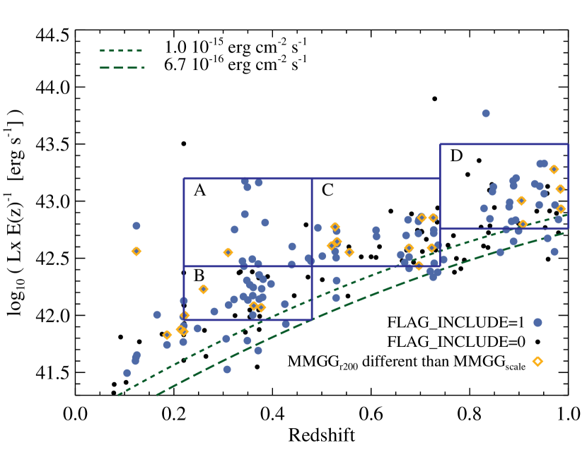
Figure 1.— Cosmos X-ray group sample as a function of redshift and $L_{X}E(z)^{-1}$, where $L_{X}$ represents X-ray luminosity and $E(z)\equiv H(z)/H_{0}$. Large blue circles indicate groups included in this analysis, and small black circles show groups that are excluded from this analysis (see text for selection flags). Yellow diamonds show systems where the centering is deemed uncertain based on the analysis of George et al. in prep., because the most massive group member lies far from the X-ray center. Blue boxes indicate the binning scheme. The redshift limits for this binning scheme are chosen to match the HOD analysis of L11.

The determination of group centers is an important and non-trivial task, especially since these structures do not always have a visually obvious central galaxy. Mis-centering effects could lead to an underestimate of $f_{\star}$, especially if the mis-centering is large enough that the true central galaxy is excluded from the group selection for example. George et al. in prep show that weak lensing is an excellent tool that can be used to optimize centering algorithms by maximizing the stacked weak lensing signal at small radii (below about 500 kpc). For example, George et al. in prep also show that various naive centering algorithms such as the centroid of galaxy members, even if weighted by stellar mass or luminosity, is a poor tracer of the centers of dark matter halos. We use the group centers from George et al. in prep that are found to maximize the stacked weak lensing signals at small radii, namely, the most massive group galaxy located within an NFW scale radius of the X-ray centroid, denoted MMGG_scale. We note, however, that George et al. in prep have also identified a sub-set of groups (of order 20%) that host a more massive galaxy at a greater distance from the X-ray centroid than the NFW scale radius. For these groups, the weak lensing does not clearly indicate a preferred center among the two options. We include these systems in our analysis but we have tested that our results are not affected by this choice.

Group members are selected according to the following criteria:

1. $P_{\rm mem}>0.5$ where $P_{\rm mem}$ denotes the group membership probability derived in Ge11.

2. $r_{2d}<R_{500c}$ where $r_{2d}$ is the projected distance to the group center (defined hereafter by the position of the MMGG_scale).

3. Galaxies must have a stellar mass above the completeness limit of the bin in consideration (see Table 1). Stellar mass completeness limits for the group membership catalog are higher than those quoted in Section 2.1, because the group membership catalog is limited to $F814W<24.2$.

Group members are selected only within a radius of $R_{500c}$ for two reasons. Ge11 have shown that the purity of the group membership assignment drops at larger radii (see their Figure 5). By only considering galaxies at $r_{2d}<R_{500c}$, we reduce the errors due to purity corrections. In addition, most previously published work on this topic has used $r_{2d}<R_{500c}$; this choice thus facilitates comparisons with previous work (see §4.5).

Once group members have been selected following the criteria outlined above, $f_{\star}$ is derived for each group as the sum of the stellar masses of all group members associated with this group divided by the halo mass. Halo masses are derived from the X-ray luminosity following the weak lensing scaling relation of Leauthaud et al. (2010).

Although in principle more direct than the HOD method, measuring $f_{\star}$ estimates from the group catalog has systematic errors that must be corrected for. The two main effects on the measurement are:

1. The completeness and purity of the membership selection. Here we include both contamination in the group membership selection due to neighboring galaxies but also the de-projection of a spherical NFW profile. Indeed, the quantity that we are interested in is $f_{\star}$ contained within a sphere of radius $R_{500c}$ whereas our membership selection is akin to selecting galaxies in a cylinder in redshift space. We therefore include a correction factor for this de-projection.

2. The stellar mass completeness of the group membership catalog (i.e., we need to account for the contribution to $f_{\star}$ from galaxies below the completeness limit).

To derive these correction factors, we use a suite of COSMOS-like mock catalogs that have been described in Ge11. Mocks were created from a single simulation (named “Consuelo”) 420 $h^{-1}$ Mpc on a side, resolved with 1400³ particles, and a particle mass of 1.87$\times 10^{9}$ $h^{-1}$ M_⊙. This simulation can robustly resolve halos with masses above $\sim 10^{11}$ $h^{-1}$ M_⊙ which corresponds to a central galaxy stellar masses of $\sim 10^{8.5}$ $h^{-1}$ M_⊙, well-matched to our completeness limit of $F814W=24.2$ at low redshift. This simulation is part of the Las Damas suite (McBride et al. in prep). Halos are identified within the simulation using a friends-of-friends finder with a linking length of $b=0.2$, and populated with mock galaxies according to the HOD model of L11. See Ge11 for further details regarding these mock catalogs.

We derive a single overall correction factor to $f_{\star}$ due to the two effects described above. To do so, we apply the group membership selection to the mock catalog and we compare the measured value of $f_{\star}$ (in the mocks) to the true value of $f_{\star}$ (within a sphere of radius $R_{500c}$). We derive correction factors separately for the contribution to $f_{\star}$ from satellite and central galaxies. These correction factors are denoted $C_{\rm sat}$ and $C_{\rm cen}$ respectively. $C_{\rm sat}$ is defined as:

$$C_{\rm sat}=\log_{10}(M_{*}^{\rm mock\_truth}/M_{*}^{\rm mock\_sel})$$ (2)

where $M_{*}^{\rm mock\_truth}$ represents the “true” total mass from the mocks in a sphere of $R_{500c}$ and down to the completeness limit of the mocks and $M_{*}^{\rm mock\_sel}$ represents our group member selection applied to the mocks. $C_{\rm cen}$ represents the equivalent for central galaxies. The correction factors are listed in Table 2 for the three redshift bins and are at most 14%. The completeness and purity correction component of $C_{\rm sat}$ is negative (the measured value of $f_{\star}^{\rm sat}$ is higher than it should be because of contamination) whereas the stellar mass completeness component of $C_{\rm sat}$ is positive (the measured value of $f_{\star}^{\rm sat}$ must be augmented to account for satellites below our completeness limit). The magnitude of the two corrections is fairly similar, but the opposite signs mean that these corrections tend to cancel each other out. The redshift trends cause the net correction for $C_{\rm sat}$ to be negative at $z\sim 0.37$ and positive at $z\sim 0.88$.

htb Bin ID Redshift lower L_X limit upper L_X limit M_∗ completeness limit $\log_{10}($L_XE(z)^-1/erg s^-1) $\log_{10}($L_XE(z)^-1/erg s^-1) $\log_{10}$(M_∗/M_⊙) A $z_{1}=[0.22,0.48]$ 41.96 42.43 9.3 B $z_{1}=[0.22,0.48]$ 42.43 43.2 9.3 C $z_{2}=[0.48,0.74]$ 42.43 43.2 9.9 D $z_{3}=[0.74,1]$ 42.76 43.5 10.3

Table 1Group binning scheme

Table 2Correction factors for group catalog

Bin ID	Redshift	$C_{\rm sat}$	$C_{\rm cen}$
A	$z_{1}=[0.22,0.48]$	-0.029	-0.019
B	$z_{1}=[0.22,0.48]$	-0.066	-0.004
C	$z_{2}=[0.48,0.74]$	-0.047	-0.017
D	$z_{3}=[0.74,1]$	0.003	-0.017

Due to the finite mass resolution of our mock catalogs, the contribution to $f_{\star}$ from very low mass galaxies (those that are not contained in our mock catalogs) will not be included. Using Equation 1, we estimate that this contribution should only be of order 1-2$\%$, and we thus neglect it here.

4. Results

4.1. Results from the HOD method

We now calculate $f_{\star}$ using the best fit HOD parameters from L11 for each of the three redshift bins. The results are shown in Figure 2. The solid dark blue, blue, and turquoise lines show $f_{\star}$ as a function of $M_{500c}$ for $z\sim 0.37$, $z\sim 0.66$, and $z\sim 0.88$ respectively. The contribution to $f_{\star}$ from central galaxies, $f_{\star}^{\rm cen}$, is shown by the dotted red line and the contribution from satellites, $f_{\star}^{\rm sat}$, is shown by the dashed yellow line. $f_{\star}$ is dominated by central galaxies at $M_{500c}\lesssim 10^{13.2}$ M_⊙ and by satellites at $M_{500c}\gtrsim 10^{13.2}$ M_⊙. Note that $f_{\star}$ in this figure does not include ICL.

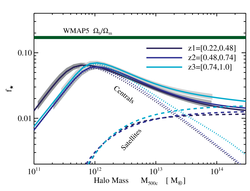
Figure 2.— Total stellar content in galaxies (not including ICL) as a function of halo mass. Results from the HOD method constrained by COSMOS data are compared to the cosmic baryon fraction measured by the Wilkinson Microwave Probe (WMAP5; $f_{b}=\frac{\Omega_{b}}{\Omega_{m}}=0.171\pm 0.009$; Dunkley et al., 2009). The results for three redshift ranges $z_{1}$, $z_{2}$, and $z_{3}$ are shown by the solid dark blue, blue, and turquoise lines respectively. The shaded region shows statistical errors only. Systematic errors are quantified in Section 4.3 (also see Figure 5). $f_{\star}$ is dominated by central galaxies at $M_{500c}\lesssim 10^{13.2}$ M_⊙ (dotted lines) and by satellites at $M_{500c}\gtrsim 10^{13.2}$ M_⊙ (dashed lines).

The redshift evolution of $f_{\star}$ has been discussed at length in L11. Briefly, the “pivot halo mass” is defined as the halo mass where $f_{\star}$ reaches a maximum ($M_{500c}\simeq 10^{12}$ M_⊙). At fixed halo mass and below the pivot halo mass scale, $f_{\star}$ increases at later epochs. This evolution can be explained by the fact that in this regime, central galaxy growth outpaces halo growth. At fixed halo mass and above the pivot halo mass scale, there is tentative evidence that $f_{\star}$ declines at later epochs. In L11, we suggest that this trend might be linked to the smooth accretion of dark matter, which brings no new stellar mass, and amounts to as much as 40% of the growth of dark matter halos (e.g., Fakhouri & Ma, 2010) and/or the destruction of satellites and a growing ICL component.

The shaded grey area in Figure 2 indicates the statistical error on $f_{\star}$. The statistical error is small compared to the systematic uncertainty associated with the actual derivation of stellar masses. We will return to this issue shortly in Section 4.3.

4.2. Results from the group catalog

We now calculate $f_{\star}$ at group scales using the COSMOS X-ray group catalog. Figure 3 shows our estimates for $f_{\star}^{\rm cen}$ (top row), $f_{\star}^{\rm sat}$ (middle row), and $f_{\star}$ (bottom row) as derived from the group catalog (the correction factors from Table 2 have been applied). Each colored data point in Figure 3 represents a measurement from one X-ray group. The thick black data point represents the mean value in each halo mass bin (see Table 1). The horizontal error corresponds to the width of the bin while the vertical error represents $\sigma/\sqrt{N_{g}}$ where $\sigma$ is the measured dispersion in the bin and $N_{g}$ is the number of groups in the bin.

The solid filled symbols in Figure 3 indicate systems for which the weak lensing analysis of George et al. in prep suggests that the group centering might be unreliable (MMGG_scale is different than MMGG_r200). We do not find a strong correlation between these systems and either halo mass or $f_{\star}$, and find that the results are unchanged if these systems are removed from the analysis.

We find excellent agreement between the HOD method and the group catalog method for $f_{\star}^{\rm cen}$ (compare the red squares to the red dotted line). Regarding $f_{\star}^{\rm sat}$, there is a small but consistent offset between the two methods (compare the yellow diamonds to the yellow dashed line). Indeed, in all three redshift bins, the $f_{\star}^{\rm sat}$ values as measured from the group catalog are higher than those derived from the HOD method by about 20% to 50%. As mentioned in the previous section, the HOD predictions for $f_{\star}^{\rm sat}$ in Figure 3 have been derived under the assumption that the distribution of satellite galaxies follows the same NFW as their parent halos. We hypothesize that the offset for $f_{\star}^{\rm sat}$ seen in Figure 3 might indicate that either a) the satellite mass distribution has different concentration than the dark matter or b) the satellite mass distribution varies with stellar mass (“mass segregation”). The observed level of offset, however, does not affect the main conclusions of this paper and so we leave a more detailed investigation of this effect for future work.

Overall, the two methods show a remarkable level of agreement especially considering the fact that they are subject to very different types of systematic errors. The two methods agree to within 30% for the estimated value for $f_{\star}$ at group scales.

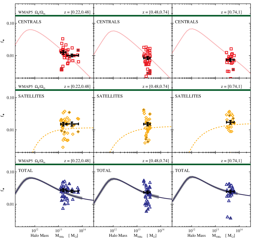
Figure 3.— Comparison between $f_{\star}$ inferred from our HOD model with results from the COSMOS X-ray group catalog as a function of redshift. The HOD values for $f_{\star}^{\rm cen}$, $f_{\star}^{\rm sat}$, and $f_{\star}$ are shown respectively by the dotted red line, and the dashed yellow line, and solid blue line. The red squares in the three top panels show $f_{\star}^{\rm cen}$ measurements from the COSMOS X-ray group catalog (each data point represents one X-ray group) for the three redshift bins. Black data points with errors show the mean value in each bin. The horizontal error corresponds to the width of the bin while the vertical error represents $\sigma/\sqrt{N_{g}}$. Here $\sigma$ is the measured dispersion in the data and $N_{g}$ is the number of groups in the bin. Yellow diamonds in the three middle panels show $f_{\star}^{\rm sat}$, and blue diamonds in the lower three panels show $f_{\star}$=$f_{\star}^{\rm cen}$+$f_{\star}^{\rm sat}$. Grey solid points indicate systems for which the centering is ambiguous (excluding these systems does not change our results).

4.3. Systematic errors associated with $f_{\star}$ measurements

The statistical uncertainty on $f_{\star}$ (from both the HOD method or the group catalog) is much smaller than the systematic uncertainty associated with the determination of stellar masses. For example, according to Behroozi et al. (2010), the typical systematic error associated with photometric-based stellar mass estimates are of order $0.25$ dex. This systematic uncertainty arises from the choice of a stellar population synthesis (SPS) model, the choice of a dust attenuation model, and the assumed functional form of the star formation history. In addition, there are also further uncertainties due to the choice of an IMF. Further details regarding systematic errors in stellar mass measurements can be found in Behroozi et al. (2010) and Conroy et al. (2009).

In this section, we attempt to quantify how the systematic errors described above might translate into an uncertainty on $f_{\star}$. Note that the aim here is only to provide a first attempt to discuss systematic errors on $f_{\star}$ due to uncertainties in stellar mass estimates (to our knowledge, this has not yet been quantified). We will make certain assumptions that will undoubtedly need to be refined in future work. We focus on the low redshift results here ($z\lesssim 0.4$) because the method used here relies on the availability of a large number of published SMFs.

To begin with, we note that the SMF provides the strongest observational constraints on the HOD model of L11. The other two observables used by L11 (clustering and galaxy-galaxy lensing) contain additional information, but this is less dominant than the information from the SMF. In this paper, we will therefore make the simplifying assumption that the main source of systematic error in the determination of $f_{\star}$ is due to uncertainties related to the SMF. Under this assumption, the task of determining systematic errors on $f_{\star}$ now becomes one of determining systematic errors on the observed SMF. We consider two distinct sources of error for the SMF:

1. A systematic error due to the choice of an IMF. In this paper, we specifically consider the Salpeter and the Chabrier IMF (Salpeter, 1955; Chabrier, 2003). To first order, the choice of a Chabrier versus a Salpeter IMF, yields masses that are lower by about 0.25 dex. For simplicity, we will assume here that we can simply convert between these two IMFs using a difference of 0.25 dex and we will refer to this difference as the “IMF systematic error on the SMF”. Note that another IMF that is often considered is the Kroupa IMF (Kroupa, 2001). The Kroupa IMF yields stellar masses that are larger than a Chabrier IMF by about 0.05 dex. We neglect any possible variations of the IMF with either galaxy type and/or redshift but note that this is another potential (and currently poorly determined) source of systematic error on $f_{\star}$.

2. All other sources of systematic error on the SMF, for example, those due to the choice of a SPS model, the choice of a dust attenuation model, and the assumed functional form of the star formation history. We will refer to these together as the “non-IMF systematic errors on the SMF”.

To estimate the non-IMF systematic errors, we consider a compilation of various published SMFs at $z<0.4$. Figure 4 shows an ensemble of low-z ($z<0.4$) mass functions from COSMOS (Drory et al., 2009; Leauthaud et al., 2011b) and from the SDSS (Panter et al., 2007; Baldry et al., 2008; Li & White, 2009). All mass functions in Figure 4 have been converted to our assumed value of $h=0.72$ and to a Chabrier IMF. Observed variations between these different mass functions are due to a combination of systematic error, measurement error, sample variance, and redshift evolution. We will adopt a conservative approach and assume that all the observed variation in Figure 4 is due to non-IMF systematic errors in the determination of stellar masses (this is an assumption that will need to be improved on in future work). We define a lower envelope and an upper envelope that is designed to encompass the observed range of SMFs. This is shown by the grey shaded region in Figure 4. In what follows, we assume that this grey shaded region represents the non-IMF systematic errors on the SMF. There is, however, one caveat with this method. Our non-IMF systematic error margin might be underestimated due to the fact that not all SPS models are represented by the set of SMFs shown in Figure 4. For example, the SPS models of Maraston (2005) are not represented in Figure 4. To date, however, there are no published $z<0.4$ SMFs that have used the Maraston (2005) models. We therefore simply note that this is a limitation with our current method that needs to be improved on in future work.

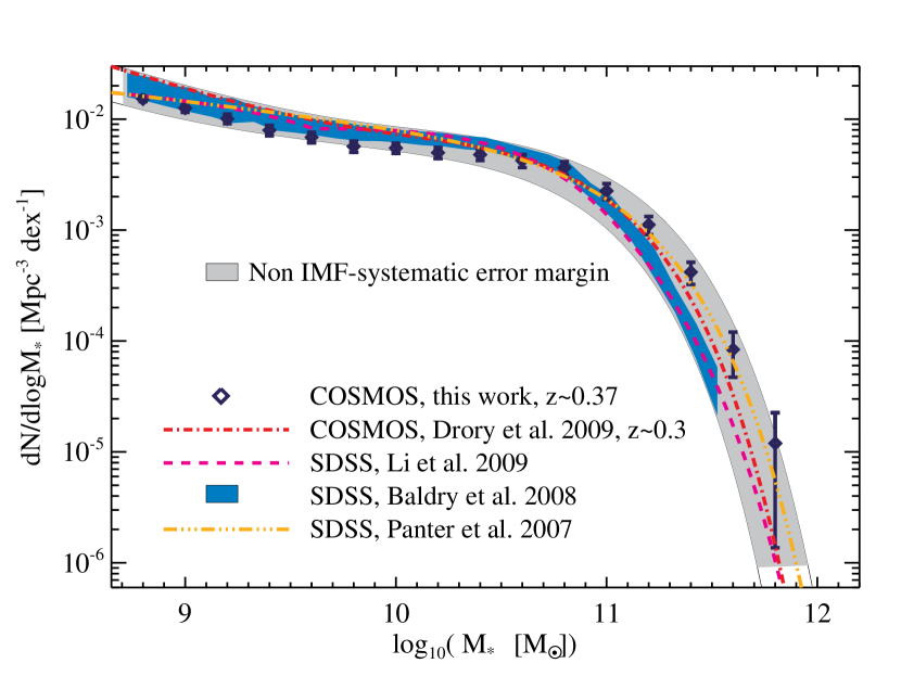
Figure 4.— Compilation of stellar mass functions at $z<0.4$. Systematic error on the SMF not including the IMF is indicated by the shaded grey region. Variation due to measurement error, sample variance between surveys, and redshift evolution is implicitly included, but we do not explore the full range of SPS models and SPS model parameters.

The next step is to understand how these non-IMF errors on the SMF might translate into a systematic error on $f_{\star}$. At present, the HOD model of L11 can only be used in conjunction with clustering and galaxy-galaxy lensing measurement. For this reason, we do not use the L11 HOD method for this step. Instead, we will adopt an “abundance matching” methodology that assumes there is a monotonic correspondence between halo mass (or circular velocity) and galaxy stellar mass (or luminosity) (e.g., Kravtsov et al., 2004; Vale & Ostriker, 2004; Tasitsiomi et al., 2004; Vale & Ostriker, 2006; Conroy et al., 2006; Conroy & Wechsler, 2009; Moster et al., 2010; Behroozi et al., 2010; Guo et al., 2010). Abundance matching techniques are generally designed to fit the SMF alone and have fewer free parameters than the HOD method. We follow the abundance matching techniques of Behroozi et al. (2010), using $M_{500c}$ halo masses, using both the upper and the lower limits of the grey shaded region in Figure 4. The abundance matching results are then reported in Figure 5 as the non-IMF systematic error margin for $f_{\star}$ (solid light grey region). The systematic errors margin for $f_{\star}$ assuming a Salpeter IMF are estimated by shifting this region upwards by 0.25 dex in stellar mass (hashed region in Figure 5).

In Figure 5, the COSMOS results are slightly higher than our non-IMF systematic error margin in Figure 5 at $M_{500c}>10^{13}$ M_⊙. This is due to the fact that the HOD method of L11 and the abundance matching method of Behroozi et al. (2010) yield slightly different predictions for $f_{\star}$ as function of halo mass; this is discussed further in the following section.

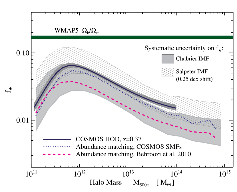
Figure 5.— Systematic error on $f_{\star}$ due to uncertainties in stellar mass estimates. The dark blue line shows the COSMOS HOD result at $z\sim 0.37$. The dotted blue line shows $f_{\star}$ derived by applying the same abundance matching technique as Behroozi et al. (2010) to the COSMOS $z\sim 0.37$ SMF. The HOD method and the abundance matching method yield slightly difference results at the 15% to 20% level. The dashed magenta line shows $f_{\star}$ as measured by Behroozi et al. (2010) by abundance matching to the Li & White (2009) SDSS SMF. The difference between the COSMOS HOD result (dark blue solid line) and the Behroozi et al. (2010) result (dashed magenta line) is largely driven by differences between the COSMOS mass function and the Li & White (2009) mass function (see Figure 4). The solid light grey region shows our the systematic error margin for $f_{\star}$, assuming a Chabrier IMF. The fact that the COSMOS results lie above this region at $M_{500c}>10^{13}$ $M_{\odot}$ is due to a $15\%$ model uncertainty between the HOD method and the abundance matching method. The hashed region shows the systematic error margin for $f_{\star}$ assuming a Salpeter IMF (note that the hashed region simply corresponds to a 0.25 dex upward shift of the solid light grey region).

4.4. Comparison with the abundance matching results of Behroozi et al. (2010)

Behroozi et al. (2010) have derived constraints on $f_{\star}$ (see their Figure 10) by abundance matching to the SDSS SMF of Li & White (2009). Figure 5 shows these results, here translated to $M_{500c}$ halo masses (magenta dashed line) and assuming a Chabrier IMF. The Behroozi et al. (2010) results yield a lower amplitude for $f_{\star}$ than the L11 COSMOS results. This is largely driven by differences between the COSMOS mass function and the Li & White (2009) mass function (shown in Figure 4).

In order to investigate how much of these differences are in fact due to differences in the assumed stellar mass function, we have applied the abundance matching technique of Behroozi et al. (2010) to the COSMOS $z\sim 0.37$ SMF. This is shown as the blue dotted line in Figure 5. This can then be directly compared with the L11 HOD results. We find that the HOD results in roughly $15$% higher values for all halo masses than the abundance matching technique shown here.

There are several possible sources for the 15% discrepancy between the HOD and abundance matching methods. One possibility is that the weak lensing and/or clustering is providing more information in the HOD analyses than is available given the stellar mass function alone, and that this information pushes the values slightly higher. Another potential issue is that conversions have been made in each case to use $M_{500c}$ halo masses (HOD results were calculated initially using $M_{200b}$ and abundance matching was done using $M_{vir}$); these conversions necessarily make assumptions about the radial profiles of satellites which may be inaccurate at the several percent level. Another possibility is that the abundance matching method might suffer from satellite incompleteness in the N-body simulations (see e.g. Wu et al. in prep), however, this is unlikely to be important below the group mass scale. We leave tracking down the exact source of the difference to future work, and simply note that there is roughly a $15$% level uncertainty in the determination of the non-IMF systematic uncertainty on $f_{\star}$ due to the method used to derive $f_{\star}$ from the SMF. Overall, the difference between L11 and Behroozi et al. (2010) is consistent with our systematic error margin for $f_{\star}$, and these differences do not impact any of our conclusions significantly.

4.5. Comparison with previous results from group and cluster catalogs

We now compare our $f_{\star}$ measurements with two recently published results from Gonzalez et al. (2007) (hereafter “Gz07”) and Giodini et al. (2009) (hereafter “Gi09”) which have been derived using group and cluster catalogs. Figure 6 shows our predictions for $f_{\star}$ as a function of $M_{500c}$ compared to the measurements of Gz07 and Gi09. In both cases, our results suggest significantly lower values for $f_{\star}$ than reported by either of these previous studies. We now provide a more detailed comparison with both Gz07 and Gi09 and discuss possible explanations for the source of the discrepancy.

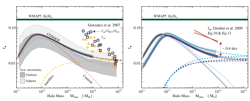
Figure 6.— Same as Figure 2, now including $f_{\star}$ measurements from Gz07 (left panel) and Gi09 (right panel). The solid light grey region in the left panel shows our the systematic error margin for $f_{\star}$, assuming a Chabrier IMF (see $\S$ 4.3). The hashed region shows the systematic error margin for $f_{\star}$ assuming a Salpeter IMF. Yellow diamonds in the left hand panel represent data-points from Gz07 for the satellite contribution to $f_{\star}$. This component can be directly compared to our low redshift satellite term (yellow dash-dash line). The total stellar mass fraction from Gz07 is shown by the blue squares ($f_{\star}^{\rm sat}$+$f_{\star}^{\rm BCG}$+$f_{\star}^{\rm ICL}$). Note that our predictions do not include the ICL contribution: our blue solid line corresponds to $f_{\star}^{\rm sat}$+$f_{\star}^{\rm BCG}$. The right panel shows the total galaxy stellar mass fraction ($f_{\star}^{\rm sat}$+$f_{\star}^{\rm BCG}$, red solid line) measured by Gi09. The Gi09 fit is averaged over all groups at $z<1$ and so is most comparable to our $z_{2}$ bin (solid blue line). In both cases, our results suggest significantly lower values for $f_{\star}$ than reported by either of these previous studies.

4.5.1 Comparison with Gonzalez et al. (2007)

The left panel of Figure 6 shows the comparison of our low-z results with Gz07. Yellow diamonds show estimates from Gz07 for the contribution to $f_{\star}$ from satellite galaxies whereas dark blue squares show the total stellar fraction ($f_{\star}^{\rm sat}$+$f_{\star}^{\rm BCG}$+$f_{\star}^{\rm ICL}$). The yellow diamonds in Figure 6 are therefore directly comparable to our prediction for $f_{\star}^{\rm sat}$ which is shown by the yellow dash-dash line. Gz07 find that $f_{\star}^{\rm sat}$ increases towards lower halo masses whereas we predict the opposite trend. It is clear from this figure that a large fraction of the observed discrepancy is due to the $f_{\star}^{\rm sat}$ component (and not so much to $f_{\star}^{\rm BCG}$ or $f_{\star}^{\rm ICL}$). We will now investigate the source of this difference in further detail.

To estimate stellar masses, Gz07 have used a Cousins I-band mass-to-light ratio ($M/L_{I}=3.6$) calibrated from the dynamical modeling of 2-d kinematic data from Cappellari et al. (2006). The Cappellari et al. (2006) sample is comprised of early type galaxies from the SAURON sample (Bacon et al. 2001). We note two important caveats with this approach:

1. The SAURON galaxy sample is comprised solely of elliptical (E) and lenticular (S0) galaxies which have larger $M/L$ values on average than intermediate and late type galaxies. If the early type fraction increases with halo mass as suggested by several studies (e.g., Weinmann et al., 2006; Hansen et al., 2009; Wetzel et al., 2011), then this could explain both why Gz07 find a steeper slope and a higher amplitude than we do for $f_{\star}^{\rm sat}$ at group scales.

2. The $M/L$ ratios presented in Cappellari et al. (2006) are dynamical (i.e total) and are therefore sensitive to the dark matter fraction within the effective radius ($R_{e}$). The dynamical mass-to-light ratios in Cappellari et al. (2006) might therefore be biased high by up to $30\%$ compared to the stellar mass-to-light ratios (see Figure 17 in Cappellari et al. 2006 for example).

We now investigate the mass-to-light ratios of our group members compared to the value used by Gz07. For this exercise, we consider group members from the membership catalog of Ge11 in our two low redshift bins (bins A and B in Figure 1). We derive Subaru $i^{+}$-band mass-to-light ratios from our stellar mass catalog using the absolute $i^{+}$-band AB magnitude that is provided by the COSMOS photoz catalog. For this exercise we adopt an AB solar luminosity of $M_{\rm sun}=4.54$. Figure 7 shows the $M/L_{i^{+}}$ values for COSMOS group members. We use unextincted rest frame magnitudes from the COSMOS photoz catalog to divide the histogram in Figure 7 by galaxy color. More specifically, we define galaxy color as $C=M(NUV)-M(R)$ where $M(NUV)$ and $M(R)$ are the unextincted rest-frame template magnitudes in the near-ultraviolet and the R bands defined in Ilbert et al. (2010). We adopt the same division as in that paper, namely:

$C<1.2$ “high activity” or “blue”

$1.2<C<3.5$ “intermediate activity” or “intermediate”

$C>3.5$ “quiescent” or “red”

We compute the difference in magnitudes between our Subaru $i^{+}$ filter and a Cousins I filter for a range of stellar population templates. We find that a Cousins $M/L_{I}=3.6$ corresponds to a Subaru $i^{+}$ mass-to-light ratio of $3.67<M/L_{i+}<4.1$ (the exact value depends on galaxy color). These values are represented in Figure 7 by the hashed magenta region.

Figure 7 shows that the stellar masses inferred by using a similar $M/L$ as Gz07 are larger than our SED stellar masses by a factor of 2 to 10 (assuming a Chabrier IMF). The difference is particularly large for active and intermediate type galaxies. The large spread observed in Figure 7 highlights the fact that the group population is not well represented by any single $i^{+}$-band $M/L_{i+}$ ratio value. Part of the observed spread can also be explained by the sensitivity of the $i^{+}$-band luminosity to recent star formation, underscoring the need for NIR data to more accurately determine galaxy stellar mass. The differences between our mass-to-light ratios and the value used by Gz07 is reduced by assuming a Salpeter IMF (Figure 7, right panel). Even with a Salpeter IMF, however, the Gz07 M/L ratio is still well above the mean M/L ratio of our galaxy sample. This is likely to be due to the fact that the Cappellari et al. (2006) mass-to-light ratios are dynamical and are thus sensitive to dark matter in addition to stellar mass.

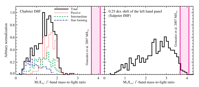
Figure 7.— Left: $i^{+}$-band mass-to-light ratios of low-z group members as a function of galaxy color as inferred from our stellar mass estimates (Chabrier IMF). The mass-to-light ratio used by Gz07 is shown by the hashed magenta region (there is a spread in values due to to conversion from Cousins I to Subaru $i^{+}$). Assuming a Chabrier IMF, the stellar masses inferred by using the Gz07 $M/L_{i^{+}}$ are larger than ours by a factor of 2 to 10. The difference is particularly large for active (blue dash-dot line) and intermediate type (green dashed line) galaxies. Right: $i^{+}$-band mass-to-light ratios assuming stellar masses are increased by 0.25 dex. To first order, these are the mass-to-light ratios expected for a Salpeter IMF. The difference is reduced by assuming a Salpeter IMF but the Gz07 M/L ratio is still well above the mean M/L ratio of our group galaxy sample.

Another important fact worth highlighting in Figure 7 is that a non negligible fraction of group members are star forming/intermediate type galaxies (also see Ge11 who find that the quenched fractions in groups is of order 40% to 60% at $z<0.5$). Note however that Figure 7 does not include the corrections described in Section 3.2 for de-projection or the completeness and purity of the membership selection. These corrections were derived as adjustments to the total $f_{\star}$ from mock catalogs that do not distinguish quiescent galaxies from active ones, so we cannot directly apply them to the separate galaxy types in Figure 7. To address the possibility of color-dependent contamination of the group sample, we can test the purity and completeness of the membership selection using a subsample of galaxies with spectroscopic redshifts as done in Ge11. The COSMOS spectroscopic redshift sample, however, is dominated by zCOSMOS “bright” galaxies with $F814W<22.5$ and is therefore not representative of our group membership sample ($F814W<24.2$). This will induce a degree of uncertainty that can only be reduced with deeper and more representative spectroscopic data and/or more representative mock catalogs. Having noted this caveat, we use this approach to compute the completeness and purity of the membership selection within $R_{500c}$ and as a function of galaxy type. We find that the group populations of red, green, and blue galaxies are overestimated by 14%, 20%, and 30% respectively. After applying these correction factors to groups in bins A and B (and for galaxies above our stellar mass completeness limit), we find that the mean red fraction at $z<0.48$ is roughly 50%. So while we do see some added contamination of our group member sample among blue galaxies, they still represent a significant part of the population. Studies that aim to compute $f_{\star}$ must take this varied group population into account. It is clear that assuming that all group members are quiescent could lead to large biases in $f_{\star}$ estimates.

Finally, we now investigate the impact of using a single mass-to-light value similar to the one use by Gz07. For this exercice we adopt a single value of $M/L_{i^{+}}=3.8$ and we neglect the small color dependance of the $M/L$ conversion from Cousins I to Subaru $i^{+}$ (see Figure 7). Using the COSMOS group catalog, we re-compute $f_{\star}^{\rm sat}$ using the absolute $i^{+}$-band AB magnitude provided by the COSMOS photoz catalog and a mass-to-light ratio of $M/L_{i^{+}}=3.8$ to derive stellar masses. Here, we only consider $f_{\star}^{\rm sat}$. Because our analysis does not include ICL, we cannot compare with the Gz07 $f_{\star}^{\rm BCG}$+$f_{\star}^{\rm ICL}$ component (these were measured together as a single component by Gz07). However, as noted in Figure 6, most of the discrepancy between our results and Gz07 occurs for $f_{\star}^{\rm sat}$. Figure 8 shows that we are able to qualitatively reproduce the Gz07 $f_{\star}^{\rm sat}$ using our data and $M/L_{i^{+}}=3.8$. Note however that the halo mass range and redshift range of our sample does not exactly match Gz07 and so Figure 8 is not exactly a one-to-one comparison. However, the fact that we obtain similar $f_{\star}^{\rm sat}$ values as Gz07 strongly suggests that the primary cause of the discrepancy is due the fact that $M/L_{i^{+}}=3.8$ largely overestimates the stellar masses of group members compared to our full SED fitting technique.

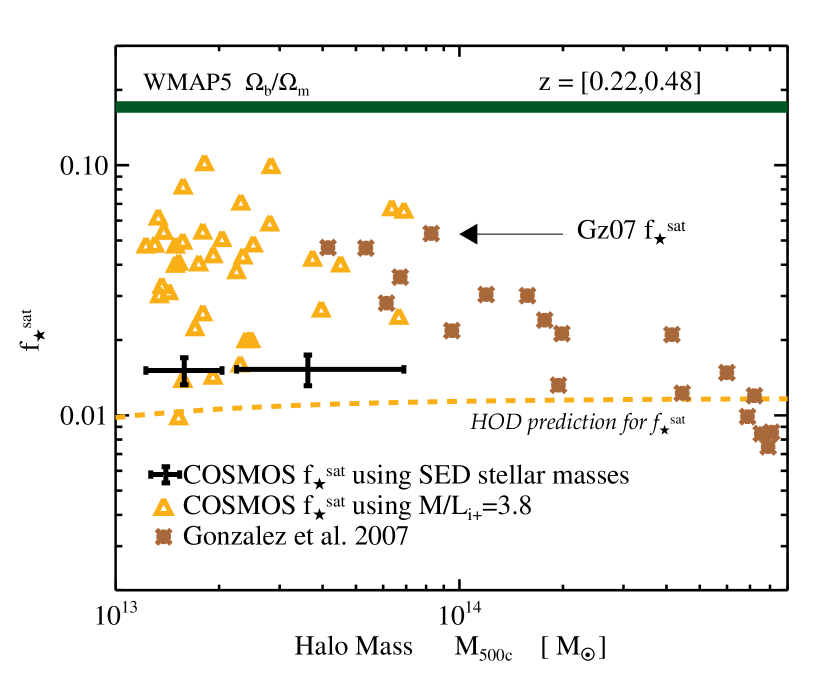
Figure 8.— Impact of mass-to-light ratio assumptions on the fraction of stars in satellites, $f_{\star}^{\rm sat}$. In addition to the default values from our group catalog (black error bars), values obtained from our group catalog using a similar $i^{+}$-band mass-to-light ratio as Gz07 ($M/L_{i^{+}}=3.8$) are shown (yellow triangles). In detail the two samples are not directly comparable because our sample has lower halo masses and is at higher redshifts than Gz07. However, the fact that the Gz07 results are qualitatively reproduced using $M/L_{i^{+}}=3.8$ suggests that the derivation of stellar masses is the primary cause of the observed difference between our results and Gz07.

4.5.2 Comparison with Giodini et al. (2009)

Gi09 have used the COSMOS data and an earlier version of our X-ray catalog to derive $f_{\star}$. Since we use the same data set and a similar group catalog, our results are directly comparable. The right panel of Figure 6 shows the comparison of our results with Gi09. Since Gi09 report the average over all groups at $z<1$, their results are most comparable with our $z_{2}$ redshift bin. To estimate stellar masses, Gi09 have used a galaxy-type dependent stellar mass-to-$K_{s}$ band luminosity ratio derived by using the analytical relation from Arnouts et al. (2007) assuming a Salpeter IMF. However, as pointed out by Ilbert et al. (2010), the Arnouts et al. (2007) $M/L_{K_{s}}$ relation was only calibrated for massive galaxies. In practice the K-band mass-to-light ratio varies with galaxy age and color. Thus the Arnouts et al. (2007) $M/L_{K_{s}}$ relation overestimates the stellar masses of low mass galaxies. Ilbert et al. (2010) have shown that the Arnouts et al. (2007) mass estimates contain galaxy-color dependent biases compared to SED fitting techniques (see their Figure 28). For example, Ilbert et al. (2010) find that the Arnouts et al. (2007) masses are biased high by more than 0.3 dex for star forming galaxies with $\log_{10}(M_{*}/M_{\odot})<9.5$. Thus, including these galaxies will lead to an overestimate of $f_{\star}$.

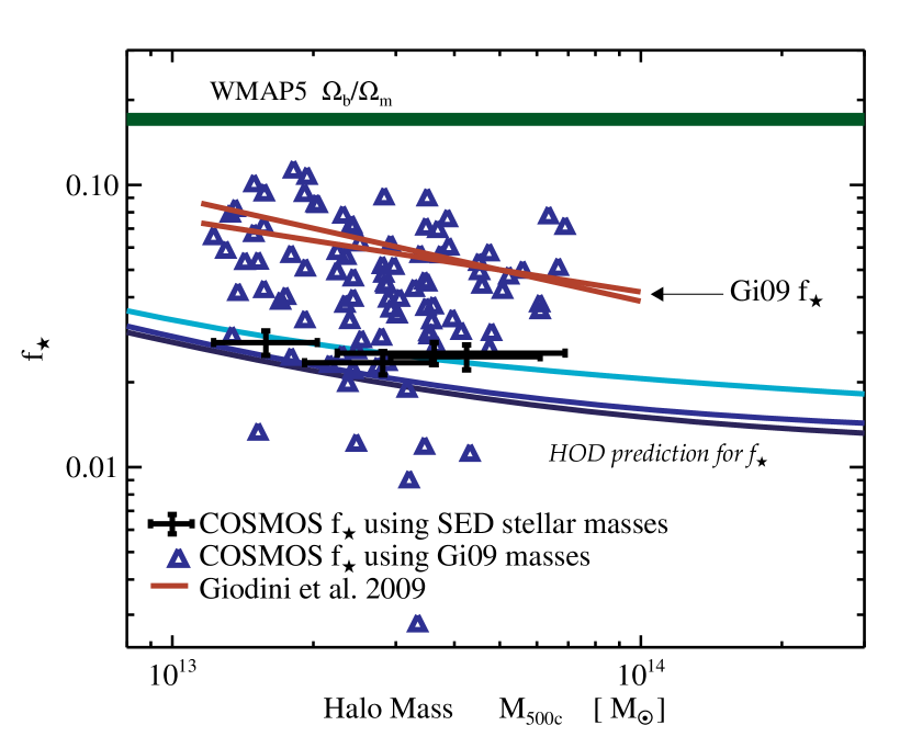
Figure 9.— Impact of stellar mass estimates on $f_{\star}$. In addition to the default values from our group catalog (black error bars), values obtained from our group catalog using the same Arnouts et al. (2007) stellar mass estimates as Gi09 are shown (blue triangles). These are in qualitative agreement with the Gi09 results (red lines), indicating that the assumptions about stellar masses are the primary source of the difference between the two sets of results.

Since the Gi09 results are based on COSMOS data, we can make a direct comparison between their mass estimates and ours. We match our galaxy catalog with the photoz catalog that was used by Gi09. We then recompute $f_{\star}$ from our catalog using the same procedure as in Section 4.2 but using the Arnouts et al. (2007) masses and the results are shown in Section 4.2. For this exercise we have used the same redshift and halo mass bins as in Section 4.2 (see Table 1). Note however that we do not apply the purity/completeness and de-projection correction factors here. Indeed, since the Gi09 stellar masses are different than ours, we would need a new set of mock catalogs to perform this correction. The correction values however are typically only of order 5 to 14% and are much smaller than difference between our results and Gi09 (a factor of $\sim$2.5). Neglecting these correction factors here should therefore not change our main conclusions.

Figure 9 shows that we obtain roughly similar values for $f_{\star}$ as Gi09 when we use the Arnouts et al. (2007) masses. In detail, however, we do not exactly find the same mean values as a function of halo mass as Gi09 but our methods are sufficiently different (Ge11 use a Bayesian probabilistic method whereas Gi09 use a background subtraction method) that this is not too unexpected. Part of the observed difference in Figure 9 is due to the fact that Gi09 use a Salpeter IMF whereas we use a Chabrier IMF (this accounts for about 0.25 dex). The remaining difference (about 0.15 dex) is probably due to a combination of differences in the techniques that we have used and to differences in stellar mass estimates.

5. Discussion and Conclusions

In this paper we have derived the total stellar mass fraction, $f_{\star}$, as a function of host halo mass from $z=0.2$ to $z=1$ using HOD methods, abundance matching methods, and direct estimates from group catalogs. Our stellar masses are derived from full SED fitting to multi-band photometry (including K-band) from the COSMOS survey. Assuming a Chabrier IMF, we find significantly lower estimates for $f_{\star}$ at group scales than previous work. Including (non-IMF) systematic errors on stellar masses, our analysis suggests that $0.012\lesssim f_{\star}\lesssim 0.025$ at $M_{500c}=10^{13}$ M_⊙ and $0.0057\lesssim f_{\star}\lesssim 0.015$ at $M_{500c}=10^{14}$ M_⊙. We will make files available upon request including our $f_{\star}$ estimates and the associated systematic uncertainties. Our main results are as follows:

1. Assuming a Chabrier IMF, we find that previously published estimates of $f_{\star}$ on group scales could be overestimated by a factor of two to five. This discrepancy is only partially reduced by assuming a Salpeter IMF. We investigate the cause of this discrepancy and find that a large fraction of the observed difference can be explained by the use of over-simplistic mass-to-light ratio estimates.

2. We show that galaxies in groups are a mixed population of quiescent, intermediate, and star forming galaxies. As a consequence, galaxies in groups are not well represented by any single $M/L$ ratio value. The assumption that all galaxies in groups are quiescent, for example, will lead to biases in $f_{\star}$ estimates.

3. We quantify the systematic uncertainty on $f_{\star}$ using abundance matching methods and show that the statistical uncertainty on $f_{\star}$ ($\sim 10$%) is currently dwarfed by systematic uncertainties associated with stellar mass measurements ($\sim 45$% excluding IMF uncertainties). We provide first estimates for the systematic error margin on $f_{\star}$ due to uncertainties in stellar mass measurements. While we have tried to provide a conservative estimate for these systematic errors, it is also clear that this is a non-trivial task that will require further investigation. One aspect in particular that could be improved on in this respect would be to consider a larger set of SMFs that cover a more representative range of SPS models than we have used here.

4. While direct measurements of $f_{\star}$ using group and cluster catalogs are necessary and important, HOD and abundance matching methods can probe $f_{\star}$ over a much wider halo mass range than possible using group and cluster catalogs. For example, in COSMOS, HOD methods allows us to probe $f_{\star}$ down to the stellar mass completeness limit of the survey ($M_{*}\sim 7\times 10^{8}$ M_⊙ and $M_{h}\sim 10^{11}$ M_⊙ at $z=0.37$). In COSMOS, we show that the HOD method and the group catalog method are in good overall agreement but exhibit some small but interesting differences regarding the contribution to $f_{\star}$ from satellite galaxies ($f_{\star}^{\rm sat}$).

5. Using identical data sets, we find that the HOD method of Leauthaud et al. (2011b) and the abundance matching method of Behroozi et al. (2010) agree to within 15% in terms of determining $f_{\star}$. Identifying the cause of remaining small differences between the two methods will require further investigation, but these small differences do not affect the main conclusions of this paper.

Our finding that the total stellar fraction in groups is lower than previously estimated has interesting implications for the thermodynamic history of the intra-group gas. In simulations, the relative proportions of gas mass to stellar mass are directly related to the efficiency of cooling, star formation, and AGN feedback (e.g., Kravtsov et al., 2005; Puchwein et al., 2008; Bode et al., 2009; Puchwein et al., 2010). Suppressed gas mass fractions at small radii might indicate that gas has been removed from the centers of groups and clusters by non gravitational processes. For example, recent simulations from McCarthy et al. (2011) have suggested that low entropy gas might be ejected from the progenitors of present-day groups by AGN feedback at high redshift (primarily $2<z<4$) at the epoch when super-massive black holes are in quasar mode. On the other hand, low gas mass fractions might also be exactly compensated for by $f_{\star}$+$f_{\rm ICL}$ in such a way that the total baryon fraction is constant with halo mass and with halo radius. Discriminating between these two scenarios is key towards understanding how much gas may have been ejected from these systems.

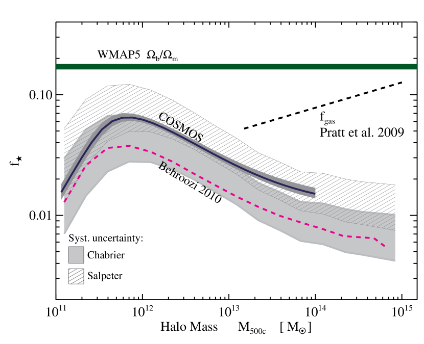
Figure 10.— Comparison of our $f_{\star}$ estimates with the mean gas mass fraction from Pratt et al. (2009). Even assuming a Salpeter IMF, our measurements imply that the total stellar content of dark matter halos is always lower than the gas mass fraction for halos above $10^{13}M_{\odot}$ and for $r<R_{500c}$.

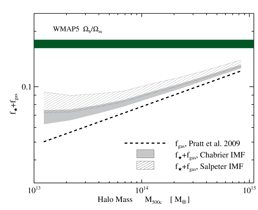
Figure 11.— Sum of the stellar fraction $f_{\star}$ and gas fraction $f_{\rm gas}$, where $f_{\rm gas}$ is the mean gas mass fraction taken from Pratt et al. (2009). The solid grey region shows the systematic error margin for $f_{\star}$+$f_{\rm gas}$ assuming a Chabrier IMF. The grey hashed region shows the systematic error margin for $f_{\star}$+$f_{\rm gas}$ assuming a Salpeter IMF.

In Figure 10, we have compared our results with the mean gas mass fraction ($f_{\rm gas}$) from Pratt et al. (2009), computed from a compilation of data from Arnaud et al. (2007), Vikhlinin et al. (2006), and Sun et al. (2009). This result demonstrates that $f_{\star}$ is always lower than $f_{\rm gas}$ for halos above $10^{13}M_{\odot}$, for the assumption of either a Salpeter or Chabrier IMF. Figure 11 shows the sum of $f_{\star}$ and $f_{\rm gas}$. Here the solid grey region indicates the systematic error margin for $f_{\star}$+$f_{\rm gas}$ assuming a Chabrier IMF; the grey hashed region shows the systematic error margin for $f_{\star}$+$f_{\rm gas}$ assuming a Salpeter IMF. Even in the latter case, we find a shortfall in $f_{\star}$+$f_{\rm gas}$ compared to the cosmic mean, which increases towards lower halos masses.

It is important to note that Figure 11 does not include a baryonic contribution from ICL. While including ICL in the baryon budget is obviously an important issue to be adressed, $f_{\rm ICL}$ estimates suffer from large uncertainties related to the choice of a $M/L$ value. For example, the ICL estimates of Gonzalez et al. (2007) assume $M/L_{I}=3.6$; Figure 7 demonstrates this is on the high end compared to $M/L_{I}$ values predicted from SPS models. Finally, we note that the main claim in this paper, that $f_{\star}$ estimates are lower than previously estimated, is dominated by the $f_{\star}^{\rm sat}$ component of $f_{\star}$.

In summary, we have presented new measurements of the stellar fraction $f_{\star}$ in groups and clusters from several complementary approaches, which we believe to be more robust than previous estimates. However, precise measurements of $f_{\star}$ are limited by our systematic uncertainties associated with stellar mass measurements. Future improvements to the $f_{\star}$ measurements presented in this paper will benefit most from efforts that lead to an improved understanding of galaxy stellar masses.

References

- Allen et al. (2008) Allen, S. W., Rapetti, D. A., Schmidt, R. W., Ebeling, H., Morris, R. G., & Fabian, A. C. 2008, MNRAS, 383, 879
- Andreon (2010) Andreon, S. 2010, MNRAS, 407, 263
- Arnaud et al. (2007) Arnaud, M., Pointecouteau, E., & Pratt, G. W. 2007, A&A, 474, L37
- Arnouts et al. (2007) Arnouts, S. et al. 2007, A&A, 476, 137
- Baldry et al. (2008) Baldry, I. K., Glazebrook, K., & Driver, S. P. 2008, MNRAS, 388, 945
- Balogh et al. (2010) Balogh, M. L., Mazzotta, P., Bower, R. G., Eke, V., Bourdin, H., Lu, T., & Theuns, T. 2010, MNRAS, 1842
- Balogh et al. (2007) Balogh, M. L., Wilman, D., Henderson, R. D. E., Bower, R. G., Gilbank, D., Whitaker, R., Morris, S. L., Hau, G., Mulchaey, J. S., Oemler, A., & Carlberg, R. G. 2007, MNRAS, 374, 1169
- Behroozi et al. (2010) Behroozi, P. S., Conroy, C., & Wechsler, R. H. 2010, ApJ, 717, 379
- Berlind & Weinberg (2002) Berlind, A. A. & Weinberg, D. H. 2002, ApJ, 575, 587
- Blanton & Roweis (2007) Blanton, M. R. & Roweis, S. 2007, AJ, 133, 734
- Bode et al. (2009) Bode, P., Ostriker, J. P., & Vikhlinin, A. 2009, ApJ, 700, 989
- Bruzual & Charlot (2003) Bruzual, G. & Charlot, S. 2003, MNRAS, 344, 1000
- Bullock et al. (2002) Bullock, J. S., Wechsler, R. H., & Somerville, R. S. 2002, MNRAS, 329, 246
- Bundy et al. (2006) Bundy, K. et al. 2006, ApJ, 651, 120
- Bundy et al. (2010) —. 2010, ApJ, 719, 1969
- Cappellari et al. (2006) Cappellari, M. et al. 2006, MNRAS, 366, 1126
- Cappelluti et al. (2009) Cappelluti, N. et al. 2009, A&A, 497, 635
- Chabrier (2003) Chabrier, G. 2003, PASP, 115, 763
- Charlot & Fall (2000) Charlot, S. & Fall, S. M. 2000, ApJ, 539, 718
- Conroy et al. (2009) Conroy, C., Gunn, J. E., & White, M. 2009, ApJ, 699, 486
- Conroy & Wechsler (2009) Conroy, C. & Wechsler, R. H. 2009, ApJ, 696, 620
- Conroy et al. (2006) Conroy, C., Wechsler, R. H., & Kravtsov, A. V. 2006, ApJ, 647, 201
- Dai et al. (2010) Dai, X., Bregman, J. N., Kochanek, C. S., & Rasia, E. 2010, ApJ, 719, 119
- Drory et al. (2009) Drory, N. et al. 2009, ApJ, 707, 1595
- Dunkley et al. (2009) Dunkley, J. et al. 2009, ApJS, 180, 306
- Elvis et al. (2009) Elvis, M. et al. 2009, ApJS, 184, 158
- Ettori (2003) Ettori, S. 2003, MNRAS, 344, L13
- Ettori et al. (2006) Ettori, S., Dolag, K., Borgani, S., & Murante, G. 2006, MNRAS, 365, 1021
- Fakhouri & Ma (2010) Fakhouri, O. & Ma, C. 2010, MNRAS, 401, 2245
- Feldmeier et al. (2004) Feldmeier, J. J., Mihos, J. C., Morrison, H. L., Harding, P., Kaib, N., & Dubinski, J. 2004, ApJ, 609, 617
- Finoguenov et al. (2007) Finoguenov, A. et al. 2007, ApJS, 172, 182
- Gallazzi et al. (2005) Gallazzi, A., Charlot, S., Brinchmann, J., White, S. D. M., & Tremonti, C. A. 2005, MNRAS, 362, 41
- Giodini et al. (2009) Giodini, S. et al. 2009, ApJ, 703, 982
- Glazebrook et al. (2004) Glazebrook, K., Abraham, R. G., McCarthy, P. J., Savaglio, S., Chen, H.-W., Crampton, D., Murowinski, R., Jørgensen, I., Roth, K., Hook, I., Marzke, R. O., & Carlberg, R. G. 2004, Nature, 430, 181
- Gonzalez et al. (2005) Gonzalez, A. H., Zabludoff, A. I., & Zaritsky, D. 2005, ApJ, 618, 195
- Gonzalez et al. (2007) Gonzalez, A. H., Zaritsky, D., & Zabludoff, A. I. 2007, ApJ, 666, 147
- Guo et al. (2010) Guo, Q., White, S., Li, C., & Boylan-Kolchin, M. 2010, MNRAS, 404, 1111
- Hansen et al. (2009) Hansen, S. M., Sheldon, E. S., Wechsler, R. H., & Koester, B. P. 2009, ApJ, 699, 1333
- Hasinger et al. (2007) Hasinger, G. et al. 2007, ApJS, 172, 29
- Hinshaw et al. (2009) Hinshaw, G. et al. 2009, ApJS, 180, 225
- Hu & Kravtsov (2003) Hu, W. & Kravtsov, A. V. 2003, ApJ, 584, 702
- Hudson et al. (2010) Hudson, M. J., Stevenson, J. B., Smith, R. J., Wegner, G. A., Lucey, J. R., & Simard, L. 2010, MNRAS, 409, 405
- Ilbert et al. (2009) Ilbert, O. et al. 2009, ApJ, 690, 1236
- Ilbert et al. (2010) —. 2010, ApJ, 709, 644
- Kauffmann et al. (2003) Kauffmann, G. et al. 2003, MNRAS, 341, 33
- Kravtsov et al. (2004) Kravtsov, A. V., Berlind, A. A., Wechsler, R. H., Klypin, A. A., Gottlöber, S., Allgood, B., & Primack, J. R. 2004, ApJ, 609, 35
- Kravtsov et al. (2005) Kravtsov, A. V., Nagai, D., & Vikhlinin, A. A. 2005, ApJ, 625, 588
- Krick et al. (2006) Krick, J. E., Bernstein, R. A., & Pimbblet, K. A. 2006, AJ, 131, 168
- Kroupa (2001) Kroupa, P. 2001, MNRAS, 322, 231
- Laganá et al. (2008) Laganá, T. F., Lima Neto, G. B., Andrade-Santos, F., & Cypriano, E. S. 2008, A&A, 485, 633
- Lagana et al. (2011) Lagana, T. F., Zhang, Y.-Y., Reiprich, T. H., & Schneider, P. 2011, ArXiv e-prints
- Leauthaud et al. (2011a) Leauthaud, A., Tinker, J., Behroozi, P. S., Busha, M. T., & Wechsler, R. H. 2011a, ApJ, 738, 45
- Leauthaud et al. (2007) Leauthaud, A. et al. 2007, ApJS, 172, 219
- Leauthaud et al. (2010) —. 2010, ApJ, 709, 97
- Leauthaud et al. (2011b) —. 2011b, ArXiv e-prints
- Li & White (2009) Li, C. & White, S. D. M. 2009, MNRAS, 398, 2177
- Lilly et al. (2007) Lilly, S. J. et al. 2007, ApJS, 172, 70
- Lin & Mohr (2004) Lin, Y. & Mohr, J. J. 2004, ApJ, 617, 879
- Lin et al. (2003) Lin, Y., Mohr, J. J., & Stanford, S. A. 2003, ApJ, 591, 749
- Maraston (2005) Maraston, C. 2005, MNRAS, 362, 799
- McCarthy et al. (2007) McCarthy, I. G., Bower, R. G., & Balogh, M. L. 2007, MNRAS, 377, 1457
- McCarthy et al. (2011) McCarthy, I. G., Schaye, J., Bower, R. G., Ponman, T. J., Booth, C. M., Dalla Vecchia, C., & Springel, V. 2011, MNRAS, 35
- Moster et al. (2010) Moster, B. P. et al. 2010, ApJ, 710, 903
- Muñoz-Cuartas et al. (2011) Muñoz-Cuartas, J. C., Macciò, A. V., Gottlöber, S., & Dutton, A. A. 2011, MNRAS, 411, 584
- Nagai & Kravtsov (2005) Nagai, D. & Kravtsov, A. V. 2005, ApJ, 618, 557
- Navarro et al. (1997) Navarro, J. F., Frenk, C. S., & White, S. D. M. 1997, ApJ, 490, 493
- Panter et al. (2004) Panter, B., Heavens, A. F., & Jimenez, R. 2004, MNRAS, 355, 764
- Panter et al. (2007) Panter, B., Jimenez, R., Heavens, A. F., & Charlot, S. 2007, MNRAS, 378, 1550
- Peacock & Smith (2000) Peacock, J. A. & Smith, R. E. 2000, MNRAS, 318, 1144
- Pracy et al. (2005) Pracy, M. B., Driver, S. P., De Propris, R., Couch, W. J., & Nulsen, P. E. J. 2005, MNRAS, 364, 1147
- Pratt et al. (2009) Pratt, G. W., Croston, J. H., Arnaud, M., & Böhringer, H. 2009, A&A, 498, 361
- Puchwein et al. (2008) Puchwein, E., Sijacki, D., & Springel, V. 2008, ApJ, 687, L53
- Puchwein et al. (2010) Puchwein, E., Springel, V., Sijacki, D., & Dolag, K. 2010, MNRAS, 406, 936
- Ramella et al. (2004) Ramella, M., Boschin, W., Geller, M. J., Mahdavi, A., & Rines, K. 2004, AJ, 128, 2022
- Salpeter (1955) Salpeter, E. E. 1955, ApJ, 121, 161
- Scoccimarro et al. (2001) Scoccimarro, R., Sheth, R. K., Hui, L., & Jain, B. 2001, ApJ, 546, 20
- Scoville et al. (2007) Scoville, N. et al. 2007, ApJS, 172, 1
- Seljak (2000) Seljak, U. 2000, MNRAS, 318, 203
- Simionescu et al. (2011) Simionescu, A., Allen, S. W., Mantz, A., Werner, N., Takei, Y., Morris, R. G., Fabian, A. C., Sanders, J. S., Nulsen, P. E. J., George, M. R., & Taylor, G. B. 2011, Science, 331, 1576
- Sun et al. (2009) Sun, M., Voit, G. M., Donahue, M., Jones, C., Forman, W., & Vikhlinin, A. 2009, ApJ, 693, 1142
- Tasitsiomi et al. (2004) Tasitsiomi, A., Kravtsov, A. V., Wechsler, R. H., & Primack, J. R. 2004, ApJ, 614, 533
- Tinker et al. (2007) Tinker, J. L., Norberg, P., Weinberg, D. H., & Warren, M. S. 2007, ApJ, 659, 877
- Tinker et al. (2011) Tinker, J. L. et al. 2011, ArXiv e-prints
- Vale & Ostriker (2004) Vale, A. & Ostriker, J. P. 2004, MNRAS, 353, 189
- Vale & Ostriker (2006) —. 2006, MNRAS, 371, 1173
- van den Bosch et al. (2008) van den Bosch, F. C., Pasquali, A., Yang, X., Mo, H. J., Weinmann, S., McIntosh, D. H., & Aquino, D. 2008, ArXiv e-prints
- Vikhlinin et al. (2006) Vikhlinin, A., Kravtsov, A., Forman, W., Jones, C., Markevitch, M., Murray, S. S., & Van Speybroeck, L. 2006, ApJ, 640, 691
- von der Linden et al. (2010) von der Linden, A., Wild, V., Kauffmann, G., White, S. D. M., & Weinmann, S. 2010, MNRAS, 404, 1231
- Wake et al. (2011) Wake, D. A. et al. 2011, ApJ, 728, 46
- Weinmann et al. (2006) Weinmann, S. M., van den Bosch, F. C., Yang, X., & Mo, H. J. 2006, MNRAS, 366, 2
- Wetzel et al. (2011) Wetzel, A. R., Tinker, J. L., & Conroy, C. 2011, ArXiv e-prints
- Wetzel & White (2010) Wetzel, A. R. & White, M. 2010, MNRAS, 403, 1072
- White et al. (2011) White, M. et al. 2011, ApJ, 728, 126
- Zehavi et al. (2002) Zehavi, I. et al. 2002, ApJ, 571, 172
- Zehavi et al. (2005) —. 2005, ApJ, 630, 1
- Zehavi et al. (2011) —. 2011, ApJ, 736, 59
- Zheng et al. (2007) Zheng, Z., Coil, A. L., & Zehavi, I. 2007, ApJ, 667, 760
- Zheng et al. (2005) Zheng, Z. et al. 2005, ApJ, 633, 791
- Zibetti et al. (2005) Zibetti, S., White, S. D. M., Schneider, D. P., & Brinkmann, J. 2005, MNRAS, 358, 949