RIKEN-MP-28

$\beta$-ensembles for toric orbifold partition function

Taro Kimura

Department of Basic Science, University of Tokyo, Tokyo 153-8902, Japan
and
Mathematical Physics Lab., RIKEN Nishina Center, Saitama 351-0198, Japan

We investigate combinatorics of the instanton partition function for the generic four dimensional toric orbifolds. It is shown that the orbifold projection can be implemented by taking the inhomogeneous root of unity limit of the $q$-deformed partition function. The asymptotics of the combinatorial partition function yields the multi-matrix model for a generic $\beta$.

1 Introduction

The instanton counting is extensively applied to various non-perturbative aspects of the four dimensional gauge theory. In particular Nekrasov partition function [1, 2] plays an essential role not only in the four dimensional Seiberg-Witten theory [3, 4], but also the two dimensional conformal field theory. The remarkable connection between the four and two dimensional theories through the instanton partition function is called AGT relation [5], and generalized to various situations, for example, the higher rank theory [6, 7], the asymptotic free theory [8, 9, 10] and also the ALE space [11, 12, 13, 14, 15], etc.

The ALE space is given by resolving the singularity of the orbifold $\mathbb{C}^{2}/\Gamma$ [16, 17, 18]. The instanton construction [19, 20], the instanton counting [21] and the wall-crossing [22, 23] are considered in this case as well as the Euclidean space $\mathbb{R}^{4}\simeq\mathbb{C}^{2}$. Furthermore the inhomogeneous orbifold theory is discussed in terms of the AGT relation [24]: it is shown that the instanton counting on the inhomogeneous orbifold $\mathbb{C}\times\mathbb{C}/\mathbb{Z}_{r}$ is utilized to describe the theory in the presence of a generic surface operator. Not only the four dimensional theory, but also the two dimensional theory with vortices on orbifolds has been recently investigated [25].

In this paper we develop the previous result [26], and consider a systematic method to deal with the combinatorial representation of the partition function for the generic four dimensional toric orbifolds $\mathbb{C}^{2}/\Gamma_{r,s}$, whose boundary is the generic lens space $L(r,s)$. It includes the type $A_{r-1}$ ALE space as $\mathbb{C}^{2}/\Gamma_{r,r-1}=\mathbb{C}^{2}/\mathbb{Z}_{r}$. So far $\mathcal{N}=4$ theories on such a space, and also Chern-Simons theory on the lens space $L(r,s)$ have been investigated [27, 28, 29, 30]. Recently further research is done with respect to the index, and its relation to the three and two dimensional theories [31].

We can obtain the orbifold partition function by performing the orbifold projection for the standard one. However it is apparently written in a complicated form, we will show a much simpler method to assign the orbifold projection. To implement that we first lift it up to the $q$-deformed theory, and then take the root of unity limit of it, as well as the standard orbifold $\mathbb{C}^{2}/\mathbb{Z}_{r}$ discussed in Ref. [26]. The similar method is also applied to the spin Calogero-Sutherland model [32] (see also Ref. [33]).

We also discuss the $\beta$-ensemble matrix model for the toric orbifold theories. We successfully obtain the multi-matrix model with a generic $\beta$ by extracting the asymptotics of the combinatorial partition function [34, 35, 36]. The $\Omega$-background parameter is related to this parameter as $\beta=-\epsilon_{2}/\epsilon_{1}$, so that it is important to discuss the generic $\beta$-ensemble in order to consider the application to the AGT relation. When we estimate the asymptotic behavior of the combinatorial part corresponding to the matrix measure, we need the root of unity limit of the $q$-deformed Vandermonde determinant, which is the weight function for the Macdonald polynomial [37]. This suggests that we can obtain a new kind of polynomials induced from the Macdonald polynomial by taking this limit.

This paper is organized as follows. In section 2 we consider the ADHM construction for the toric orbifolds $\mathbb{C}^{2}/\Gamma_{r,s}$, and then obtain the combinatorial expression for the partition function. We will show that the root of unity limit of the $q$-deformed partition function is essential for the orbifold projection, and it is useful to introduce the basis of the fractional exclusive statistics. Section 3 is devoted to derivation of the matrix models. We obtain the $\beta$-ensemble multi-matrix model by taking the asymptotic limit of the combinatorial partition function. In section 4 we summarize the results with some discussions.

2 Instanton counting on toric orbifolds

Let us start with the generic four dimensional toric space. It is given by the quotient $\mathbb{C}^{2}/\Gamma_{r,s}$ where $\Gamma_{r,s}$ is a $\mathbb{Z}_{r}$ action labeled by the two coprime integers $(r,s)$ with $0<s<r$ as

$$\Gamma_{r,s}:~{}(z_{1},z_{2})\quad\longrightarrow\quad(\omega_{r}z_{1},\omega_{r}^{s}z_{2})$$ (2.1)

where $\omega_{r}=\exp(2\pi i/r)$ is the primitive $r$-th root of unity. This space goes to the lens space $L(r,s)$ at infinity.

The orbifold action (2.1) generates a singularity at the origin of $\mathbb{C}^{2}$. We can obtain the smooth manifold by resolving the singularity, which is called the Hirzebruch-Jung space [38]. After blowing up the singularity there are $\ell$ two-spheres characterized by the generalized Cartan matrix

$$C=\left(\begin{array}[]{ccccc}-e_{1}&1&0&\cdots&0\\ 1&-e_{2}&1&\cdots&0\\ 0&1&-e_{3}&\cdots&0\\ \vdots&\vdots&\vdots&\ddots&\vdots\\ 0&0&0&\cdots&-e_{\ell}\\ \end{array}\right)$$ (2.2)

where the self-intersection numbers $e_{i}$, $i=2,\cdots,\ell$ are obtained by expanding the rational number $r/s$ in a continued fraction form

$$\frac{r}{s}=e_{1}-{1\over\displaystyle e_{2}-{1\over\displaystyle e_{3}-{1\over\displaystyle\ddots{}~{}e_{\ell-1}-{1\over e_{\ell}}}}}$$ (2.3)

and $e_{1}$ is the smallest integer greater than $r/s$. In the case of the ALE space, namely $s=r-1$, we have $e_{i}=2$ and $\ell=r-1$. Therefore the matrix (2.2) coincides with the Cartan matrix for the type-$A_{r-1}$ Lie algebra.

We then consider the standard ADHM construction for $\mathbb{R}^{4}\simeq\mathbb{C}^{2}$ to study instanton counting before orbifolding. The ADHM equations for $k$-instanton configuration for $\mathrm{SU}(n)$ theory are given by

$$\mathcal{E}_{\mathbb{C}} := \left[B_{1},B_{2}\right]+IJ=0,$$ (2.4)

$$\mathcal{E}_{\mathbb{R}} := [B_{1},B_{1}^{\dagger}]+[B_{2},B_{2}^{\dagger}]+II^{\dagger}-J^{\dagger}J=0$$ (2.5)

where the ADHM data $(B_{1},B_{2},I,J)$ are interpreted as elements of homomorphisms,

$$B_{1},B_{2}\in\mathrm{Hom}\left(V,V\right),\qquad I\in\mathrm{Hom}\left(W,V\right),\qquad J\in\mathrm{Hom}\left(V,W\right).$$ (2.6)

The rank of the gauge group and the instanton number are encoded in dimensions of the vector spaces, dim $V=n$ and dim $W=k$, respectively. Actually, when we consider $\mathrm{SU}(n)$ theory, we had better deal with $\mathrm{U}(n)$ group, and then implement the condition for the Coulomb moduli $\sum_{l=1}^{n}a_{l}=0$. Note that this procedure is not enough for some cases: we have to factor out the $\mathrm{U}(1)$ contribution when we consider the AGT relation [5].

There is $\mathrm{U}(k)$ gauge symmetry for these ADHM data

$$\left(B_{1},B_{2},I,J\right)\quad\longrightarrow\quad\left(gB_{1}g^{-1},gB_{2}g^{-1},gI,Jg^{-1}\right),\qquad g\in\mathrm{U}(k),$$ (2.7)

and thus the instanton moduli space is given by

$$\mathcal{M}_{n,k}=\left\{(B_{1},B_{2},I,J)|\mathcal{E}_{\mathbb{C}}=0,\mathcal{E}_{\mathbb{R}}=0\right\}/\mathrm{U}(k).$$ (2.8)

The resolution of singularity of this ADHM moduli space is given by the following quotient [39],

$$\widetilde{\mathcal{M}}_{n,k}=\left\{(B_{1},B_{2},I,J)|\mathcal{E}_{\mathbb{C}}=0,\mbox{stability cond.}\right\}//\mathrm{GL}(k,\mathbb{C}).$$ (2.9)

The stability condition is interepreted as the irreducibility for the moduli space.

We then consider the action of isometries on $\mathbb{C}^{2}$ for the ADHM data

$$\left(B_{1},B_{2},I,J\right)\quad\longrightarrow\quad\left(T_{1}B_{1},T_{2}B_{2},IT_{a}^{-1},T_{1}T_{2}T_{a}J\right)$$ (2.10)

where $T_{a}=\mathrm{diag}(e^{ia_{1}},\cdots,e^{ia_{n}})\in\mathrm{U}(1)^{n}$, $T_{\alpha}=e^{i\epsilon_{\alpha}}\in\mathrm{U}(1)^{2}$. They are the torus actions coming from the symmetry of $\mathrm{U}(n)$ and $\mathrm{SO}(4)$, respectively. We have to consider the fixed point of these isometries up to gauge transformation $g\in\mathrm{U}(k)$ to perform the localization formula. Thus the orbifold action, corresponding to (2.1), on the ADHM data is

$$\Gamma_{r,s}:~{}(B_{1},B_{2},I,J)\quad\longrightarrow\quad(\omega_{r}B_{1},\omega_{r}^{s}B_{2},I,\omega_{r}^{1+s}J).$$ (2.11)

Due to the orbifold action we have to introduce decomposed vector spaces with respect to the irreducible representations of $\mathbb{Z}_{r}$,

$$W=\bigoplus_{v=1}^{r}W_{v},\qquad V=\bigoplus_{v=1}^{r}V_{v},$$ (2.12)

Here we assign the orbifold action for the gauge group element as $e^{ia_{l}}\to\omega_{r}^{p_{l}}e^{ia_{l}}$. It is just a holonomy, which characterizes the boundary condition of the gauge field. Thus the ADHM data surviving under the orbifold action can be written as

$$B_{1,v}\in\mathrm{Hom}(V_{v},V_{v+1}),\quad B_{2,v}\in\mathrm{Hom}(V_{v},V_{v+s}),\quad I_{v}\in\mathrm{Hom}(W_{v},V_{v}),\quad J_{v}\in\mathrm{Hom}(V_{v},W_{v+1+s}),$$ (2.13)

and thus we have

$$\mathcal{E}_{\mathbb{C}} \longrightarrow B_{1,v+s}B_{2,v}-B_{2,v+1}B_{1,v}+I_{v+1+s}J_{v},$$ (2.14)

$$\mathcal{E}_{\mathbb{R}} \longrightarrow B_{1,v-1}B_{1,v-1}^{\dagger}-B_{1,v}^{\dagger}B_{1,v}+B_{2,v-s}B_{2,v-s}^{\dagger}-B_{2,v}^{\dagger}B_{2,v}+I_{v}I_{v}^{\dagger}-J_{v}J_{v}^{\dagger}.$$ (2.15)

They are periodic modulo $r$ as $W_{r+1}=W_{1}$ and so on. Fig. 1 shows quiver diagrams for orbifolding ADHM data. These conditions are much complicated, and thus the whole structure of the instanton moduli space is not yet clear. Actually (2.14) and (2.15) take non-zero value after resolving the singularity. It can concern possibility of the localization method. Its availability is investigated for the case of the ALE space [21] and more generic theories [40, 41], but we have to consider this problem more explicitly. Basically we still have the isometry $\mathrm{U}(1)^{2}$ corresponding to the spatial rotation even for the orbifolds. This might ensure that we can apply the localization formula to these cases.

Figure 1: Quiver diagrams for orbifolding ADHM data: (a) $\mathbb{C}^{2}/\Gamma_{5,4}$ ( the ALE space $\mathbb{C}^{2}/\mathbb{Z}_{5}$) and (b) $\mathbb{C}^{2}/\Gamma_{5,3}$.

We then derive the combinatorial representation of the partition function. Since the characters of the vector spaces are given by

$$V=\sum_{l=1}^{n}\sum_{(i,j)\in\lambda^{(l)}}T_{a_{l}}T_{1}^{1-i}T_{2}^{1-j},\qquad W=\sum_{l=1}^{n}T_{a_{l}},$$ (2.16)

the character of the tangent space at the fixed point under the isometries, which is labeled by $n$-tuple partition $\vec{\lambda}$, turns out to be

$$\chi_{\vec{\lambda}} = -V^{*}V(1-T_{1})(1-T_{2})+W^{*}V+V^{*}WT_{1}T_{2}$$ (2.17)

$$= \sum_{l,m}^{n}\sum_{(i,j)\in\lambda^{(l)}}\left(T_{a_{ml}}T_{1}^{\lambda_{i}^{(m)}-j+1}T_{2}^{-\check{\lambda}_{j}^{(l)}+i}+T_{a_{lm}}T_{1}^{-\lambda_{i}^{(m)}+j}T_{2}^{\check{\lambda}_{j}^{(l)}-i+1}\right).$$

Here we define $a_{lm}=a_{l}-a_{m}$, $T_{a_{lm}}=e^{ia_{lm}}$, etc. We can extract the weight, and thus obtain the partition function in a combinatorial way,

$$Z_{\vec{\lambda}}=\prod_{l,m}^{n}\prod_{(i,j)\in\lambda^{(l)}}\frac{1}{a_{ml}+\epsilon_{1}(\lambda_{i}^{(m)}-j+1)-\epsilon_{2}(\check{\lambda}_{j}^{(l)}-i)}\frac{1}{a_{lm}-\epsilon_{1}(\lambda_{i}^{(m)}-j)+\epsilon_{2}(\check{\lambda}_{j}^{(l)}-i+1)}.$$ (2.18)

This is the instanton partition function [1]. The two parameters, $\epsilon_{1}$ and $\epsilon_{2}$, are called $\Omega$-background parameters, which are required for regularizing the singularities in the moduli space.

We then have the partition function for the orbifold theory by taking into account only the invariant sector under the orbifold action (2.11). Since each contribution to the character behaves under the orbifold action as

$$\Gamma_{r,s}:~{}T_{a_{ml}}T_{1}^{\lambda_{i}^{(m)}-j+1}T_{2}^{-\check{\lambda}_{j}^{(l)}+i}\quad\longrightarrow\quad\omega_{r}^{p_{ml}+\lambda_{i}^{(m)}-j+\bar{s}(\check{\lambda}_{j}^{(l)}-i)+1}T_{a_{ml}}T_{1}^{\lambda_{i}^{(m)}-j+1}T_{2}^{-\check{\lambda}_{j}^{(l)}+i}$$ (2.19)

and so on, the $\Gamma_{r,s}$-invariant sector is different for the first and the second parts in the product,

$$\frac{1}{a_{ml}+\epsilon_{1}(\lambda_{i}^{(m)}-j+1)-\epsilon_{2}(\check{\lambda}_{j}^{(l)}-i)}\quad\mbox{for}\quad p_{l}-p_{m}+\lambda_{i}^{(m)}-j+\bar{s}(\check{\lambda}_{j}^{(l)}-i)+1\equiv 0~{}(\mbox{mod}~{}r),$$ (2.20)

$$\frac{1}{a_{lm}-\epsilon_{1}(\lambda_{i}^{(m)}-j)+\epsilon_{2}(\check{\lambda}_{j}^{(l)}-i+1)}\quad\mbox{for}\quad p_{l}-p_{m}+\lambda_{i}^{(m)}-j+\bar{s}(\check{\lambda}_{j}^{(l)}-i)+\bar{s}\equiv 0~{}(\mbox{mod}~{}r),$$ (2.21)

with $\bar{s}=r-s$. Thus the partition function for $\mathrm{U}(1)$ theory on the toric orbifold is given by

$$Z_{\lambda;\Gamma_{r,s}}=\prod_{\mbox{\scriptsize$\check{\Gamma}$-inv.}\subset\lambda}\frac{1}{\lambda_{i}-j+\beta(\check{\lambda}_{j}-i)+1}\prod_{\mbox{\scriptsize$\hat{\Gamma}$-inv.}\subset\lambda}\frac{1}{\lambda_{i}-j+\beta(\check{\lambda}_{j}-i)+\beta}.$$ (2.22)

We introduce another parameter defined as $\beta=-\epsilon_{2}/\epsilon_{1}$. Here $\check{\Gamma}$- and $\hat{\Gamma}$-invariant sectors stand for the conditions shown in (2.20) and (2.21), respectively. It can be easily extended to $\mathrm{SU}(n)$ gauge theory.

These conditions to extract the $\Gamma_{r,s}$-invariant sectors are apparently complicated, but there is a simple way to implement the orbifold projection [26, 32]. To implement the orbifold projection, let us start with the standard partition function before orbifolding, and then lift it to the $q$-deformed partition function, which is interpreted as the five dimensional function,

$$Z_{\lambda}^{q}=\prod_{(i,j)\in\lambda}\frac{1}{1-q^{\lambda_{i}-j+1}t^{\check{\lambda}_{j}-i}}\frac{1}{1-q^{-\lambda_{i}+j}t^{-\check{\lambda}_{j}+i-1}}.$$ (2.23)

These $q$ and $t$ are related to the $\Omega$-background parameters as $q=e^{\epsilon_{1}}$, $t=e^{-\epsilon_{2}}=q^{\beta}$. Of course we obtain the original four dimensional function by taking the usual $q\to 1$ limit. On the other hand, by taking the root of unity limit of the $q$-deformed function, the orbifolded partition function (2.22) is automatically obtained up to constants. In this case we assign the following parametrization,

$$q\longrightarrow\omega_{r}q,\qquad t\longrightarrow\omega_{r}^{-s}q^{\beta}=\omega_{r}^{\bar{s}}q^{\beta}$$ (2.24)

and then take the limit $q\to 1$. To regularize the singular behavior at $q\to 1$, we now take into account the adjoint matter contribution whose mass parameter is given by $\mathfrak{m}$. Thus the weight function yields, for example,

$$\frac{1-\omega_{r}^{\lambda_{i}-j+\bar{s}(\check{\lambda}_{j}-i)+1}q^{\lambda_{i}-j+1+\mathfrak{m}}t^{\check{\lambda}_{j}-i}}{1-\omega_{r}^{\lambda_{i}-j+\bar{s}(\check{\lambda}_{j}-i)+1}q^{\lambda_{i}-j+1}t^{\check{\lambda}_{j}-i}}$$ (2.27)

$$\longrightarrow \left\{\begin{array}[]{ccc}\frac{\lambda_{i}-j+\beta(\check{\lambda}_{j}-i)+1+\mathfrak{m}}{\lambda_{i}-j+\beta(\check{\lambda}_{j}-i)+1}&\mbox{if}&\lambda_{i}-j+\bar{s}(\check{\lambda}_{j}-i)+1\equiv 0~{}(\mbox{mod}~{}r)\\ 1&\mbox{if}&\lambda_{i}-j+\bar{s}(\check{\lambda}_{j}-i)+1\not\equiv 0~{}(\mbox{mod}~{}r)\\ \end{array}\right..$$

If we want to extract only the contribution of the vector multiplet, we have to take the decoupling limit $\mathfrak{m}\to\infty$.

The $q$-partition function for $\mathrm{SU}(n)$ theory can be written with the cut off parameter $N^{(l)}$ for the number of entries of the partitions as follows,

$$Z_{\vec{\lambda}}^{q}=\prod_{(l,i)\not=(m,j)}\frac{(Q_{lm}q^{\lambda_{i}^{(l)}-\lambda_{j}^{(m)}}t^{j-i};q)_{\infty}}{(Q_{lm}q^{\lambda_{i}^{(l)}-\lambda_{j}^{(m)}}t^{j-i+1};q)_{\infty}}\prod_{l,m}^{n}\prod_{i=1}^{N^{(l)}}\frac{(Q_{lm}q^{\lambda_{i}^{(l)}}t^{N^{(m)}-i+1};q)_{\infty}}{(Q_{ml}q^{-\lambda_{i}^{(l)}}t^{-N^{(m)}+i};q)_{\infty}}.$$ (2.28)

Here $(x;q)_{n}=\prod_{m=0}^{n-1}(1-xq^{m})$ is the $q$-Pochhammer symbol, and the Coulomb moduli is denoted as $Q_{lm}=e^{a_{lm}}=q^{b_{lm}}$. Note that this $q$-partition function includes the infinite product, so that we have to take care of its radius of convergence. Therefore we first consider the parametrization (2.24), and then take the limit $q\to 1$. This orbifold projecting procedure is quite useful, for example, to investigate asymptotic behavior of the orbifold partition function because it can be simply given by studying asymptotics of the $q$-partition function in a usual way, and taking its root of unity limit at last.

We now comment on the relation to the explicit expressions for $\mathcal{O}_{\mathbb{P}_{1}}(-r)$, etc, which is shown in Refs. [27, 41]. They are written down in terms of the local coordinates of the resolved space. For example, in the case of $\mathcal{O}_{\mathbb{P}_{1}}(-r)$, they are given by $(z_{1}^{(1)},z_{2}^{(1)})=(z_{1}^{r},z_{1}^{-1}z_{2})$ and $(z_{1}^{(2)},z_{2}^{(2)})=(z_{1}z_{2}^{-1},z_{2}^{r})$, which are invariant under $(z_{1},z_{2})\to(\omega_{r}z_{1},\omega_{r}z_{2})$. Thus we have the instanton partition function, which is manifestly invariant under the orbifold action. This manipulation gives rise to redefinition of the partitions: if we consider $\mathrm{U}(1)$ theory for simplicity, we have $\lambda_{i}\to\lambda_{I}^{(1)},\lambda_{I}^{(2)}$, which satisfy $\lambda_{i}=r\lambda_{I}^{(1)}+I$ with $i=I$ or $\lambda_{i}=\lambda_{I}^{(2)}$ with $i=\lambda_{I}^{(2)}+rI$. Here the superscript labels the local patch of the resolved space. The expressions for $\mathcal{O}_{\mathbb{P}_{1}}(-r)$ can be obtained by these redefined variables. Anyway this connection is still complicated, thus it should be investigated in detail for further study.

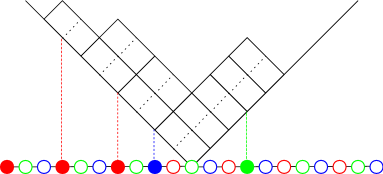
Figure 2: Decomposition of the partition $\lambda=(5,2,2,1)$ for $\mathbb{C}^{2}/\Gamma_{3,1}$. A rectangular box is required for obtaining the correspondence between the partition and the particle description with the repulsion parameter $\bar{s}=r-s$.

To treat the orbifold partition function more conveniently, we then try to decompose the partitions. In this case we introduce a slightly different way of decomposition [42, 26],

$$r(\lambda_{i}^{(l,v)}+N^{(l,v)}-i+p^{(l,v)})+v\equiv\lambda_{j}^{(l)}+\bar{s}(N^{(l)}-j)+p_{l},\qquad j=c_{i}^{(l,v)}$$ (2.29)

where $c_{i}^{(l,v)}$ stands for the mapping from the index of the divided $nr$-partition to that of the original $n$-partition. Fig. 2 shows an example for the case with the orbifold $\mathbb{C}^{2}/\Gamma_{3,1}$, namely $\bar{s}=2$.

This decomposition is based on the particle description obeying the fractional exclusive statistics [43], which is deeply related to Calogero-Sutherland model (see, for example, Ref. [33]). The parameter $\bar{s}$ stands for the strength of the repulsion between particles, and this generalized statistics goes back to the usual fermionic one in the case of the ALE space, $\bar{s}=1$. It is useful to introduce a rectangular box to obtain the correspondence between the partition and the particle description due to the repulsion parameter $\bar{s}$.

Introducing another set of variables defined as

$$\ell_{i}^{(l,v)}\equiv r(\lambda_{i}^{(l,v)}+N^{(l,v)}-i+p^{(l,v)})+b_{l}-p_{l}+v,$$ (2.30)

we finally obtain $r$-tuple partition by blending $nr$-tuple one,

$$\ell^{(v)}_{i=1,\cdots,\sum_{l=1}^{n}N^{(l,v)}}=\left(\ell_{1}^{(n,v)},\cdots,\ell_{N^{(n,v)}}^{(n,v)},\cdots,\ell_{1}^{(1,v)},\cdots,\ell_{N^{(1,v)}}^{(1,v)}\right).$$ (2.31)

We now assume $N^{(l)}={\bf N}$ and $N^{(l,v)}=N$ for simplicity. Thus the partition function is rewritten in terms of $r$-tuple partition,

$$Z_{\vec{\lambda}}^{q} = \prod_{(v,i)\not=(w,j)}\frac{(\omega_{r}^{v-w}q^{\ell_{i}^{(v)}-\ell_{j}^{(w)}+(\beta-\bar{s})(c_{j}^{(w)}-c_{i}^{(v)})};\omega_{r}q)_{\infty}}{(\omega_{r}^{v-w+\bar{s}}q^{\ell_{i}^{(v)}-\ell_{j}^{(w)}+(\beta-\bar{s})(c_{j}^{(w)}-c_{i}^{(v)})+\beta};\omega_{r}q)_{\infty}}$$ (2.32)

$$\times\prod_{l=1}^{n}\prod_{v=0}^{r-1}\prod_{i=1}^{nN}\frac{(\omega^{r-p_{l}+\bar{s}}q^{\ell_{i}^{(v)}-b_{l}+(\beta-\bar{s})({\bf N}-c_{i}^{(v)})+\beta};\omega_{r}q)_{\infty}}{(\omega^{-r+p_{l}}q^{-(\ell_{i}^{(v)}-b_{l}+(\beta-\bar{s})({\bf N}-c_{i}^{(v)}))};\omega_{r}q)_{\infty}}$$

Let $c_{i}^{(v)}$ stand for the mapping of the index from $r$-tuple to $nr$-tuple partition as before.

3 Matrix model description

We then derive matrix model description by taking asymptotic limit of the combinatorial representation of the partition function (2.32). Such an integral representation would be useful to extract the gauge theory consequences by performing the large $N$ limit analysis: the Seiberg-Witten curve is obtained from the spectral curve of the matrix model [44, 34, 26].

We now consider the following function to study the asymptotics of the partition function,

$$f_{q,t}(x)=\frac{(x;q)_{\infty}}{(tx;q)_{\infty}}.$$ (3.1)

The asymptotics of this function is almost given by the limit of $|q|\to 1$ because, when $x=e^{y}$, we have

$$f_{q,t}(x)=\prod_{n=0}^{\infty}\frac{1-e^{y+n\epsilon_{1}}}{1-e^{y+(n+\beta)\epsilon_{1}}}.$$ (3.2)

Therefore the condition $y\gg\epsilon_{1}$ corresponds to the limit $q\to 1$. This function is investigated in detail in appendix A.

Thus we now apply the result for the double root of unity limit (A.20) to the combinatorially represented partition function. Introducing the following variables

$$x_{i}^{(v)}=\frac{\ell_{i}^{(v)}}{\epsilon_{1}},$$ (3.3)

and taking the limit $\epsilon_{1}\to 0$, we then obtain the matrix model representation which captures the asymptotics of the combinatorial partition function. For the orbifold $\mathbb{C}^{2}/\Gamma_{r,s}$, we have the $r$-matrix model,

$$Z=\int\mathcal{D}\vec{X}~{}e^{-\frac{1}{\epsilon_{1}}\sum_{v=0}^{r-1}\sum_{i=1}^{N}V(x_{i}^{(v)})},$$ (3.4)

$$\mathcal{D}\vec{X}=\prod_{v=0}^{r-1}\prod_{i=1}^{N}\frac{dx_{i}^{(v)}}{2\pi}\Delta^{2}(x).$$ (3.5)

Note that we have to replace the summation over the partition with the integral of the continuous variables. This is done by inserting an auxiliary function, which has a simple pole at all integer values of the argument [34, 35, 36]. This affects on the matrix integral as just a linear shift of the matrix potential in the large $N$ limit, which can be absorbed by the counting parameter.

Let us now discuss the matrix measure and the potential function. According to (A.20), asymptotics of the first part in (2.32), which will go to the measure part of the matrix model, yields

$$\prod_{(v,i)\not=(w,j)}f_{q,t}\left(\omega_{r}^{v-w}q^{\ell_{i}^{(v)}-\ell_{j}^{(w)}+(\beta-\bar{s})(c_{j}^{(w)}-c_{i}^{(v)})}\right)$$ (3.6)

$$\simeq \prod_{(v,i)\not=(w,j)}\left[\left(1-e^{r(x_{i}^{(v)}-x_{j}^{(w)})}\right)^{(\beta-\bar{s})/r}\prod_{k=0}^{\bar{s}-1}\left(1-\omega_{r}^{v-w+k}e^{x_{i}^{(v)}-x_{j}^{(w)}}\right)\right].$$

This coincides with the following matrix measure, up to the overall factor,

$$\Delta^{2}(x) = \prod_{v=0}^{r-1}\prod_{i<j}^{N}\left[\left(2\sinh\frac{r}{2}\left(x_{i}^{(v)}-x_{j}^{(v)}\right)\right)^{2(\beta-\bar{s})/r}\prod_{k=0}^{\bar{s}-1}\left(2\sinh\frac{1}{2}\left(x_{i}^{(v)}-x_{j}^{(v)}+\frac{2\pi i}{r}k\right)\right)^{2\bar{s}}\right]$$

$$\times \prod_{v<w}^{r-1}\prod_{i,j}^{N}\left[\left(2\sinh\frac{r}{2}\left(x_{i}^{(v)}-x_{j}^{(w)}\right)\right)^{2(\beta-\bar{s})/r}\prod_{k=0}^{\bar{s}-1}\left(2\sinh\frac{1}{2}\left(x_{i}^{(v)}-x_{j}^{(w)}+\frac{2\pi i}{r}(v-w+k)\right)\right)^{2}\right].$$

We redefine the matrix size as $nN\to N$ for convenience. We ramark that $\beta$ can take a generic value, thus (LABEL:mat_meas) is interpreted as the measure part of the $\beta$-ensemble matrix model for the generic toric orbifold.

The corresponding four dimensional limit is given by

$$\Delta^{2}(x) \to \prod_{v=0}^{r-1}\prod_{i<j}^{N}\left(x_{i}^{(v)}-x_{j}^{(v)}\right)^{2(\beta-\bar{s})/r+2\bar{s}}\prod_{v<w}^{r-1}\prod_{i,j}^{N}\left(x_{i}^{(v)}-x_{j}^{(w)}\right)^{2(\beta-\bar{s})/r+2N_{\bar{s}}(v-w)},$$ (3.8)

where we define $N_{\bar{s}}(x)=\#\{k|x+k\equiv 0~{}(\mbox{mod}~{}r),k=0,\cdots,\bar{s}-1\}$.

We can easily obtain important examples from this generic result. For the case of $\bar{s}=1$, corresponding to the orbifold $\mathbb{C}^{2}/\mathbb{Z}_{r}$, we have

$$\Delta^{2}(x) = \prod_{v=0}^{r-1}\prod_{i<j}^{N}\left[\left(2\sinh\frac{r}{2}\left(x_{i}^{(v)}-x_{j}^{(v)}\right)\right)^{2(\beta-1)/r}\left(2\sinh\frac{1}{2}\left(x_{i}^{(v)}-x_{j}^{(v)}\right)\right)^{2}\right]$$

$$\times \prod_{v<w}^{r-1}\prod_{i,j}^{N}\left[\left(2\sinh\frac{r}{2}\left(x_{i}^{(v)}-x_{j}^{(w)}\right)\right)^{2(\beta-1)/r}\left(2\sinh\frac{1}{2}\left(x_{i}^{(v)}-x_{j}^{(w)}+\frac{2\pi i}{r}(v-w)\right)\right)^{2}\right].$$

This is consistent with the previous result [26]. In this time this formula is available even for generic $\beta$ while only the specific case $\beta=r\gamma+1\equiv 1$ (mod $r$), $\gamma=0,1,2,\cdots$, is investigated in the previous paper. This generalization is quite important because, in terms of AGT relation, the parameter $\beta$ plays a crucial role in both of the four dimensional and two dimensional theories.

The second is the case $\bar{s}=r$, corresponding to the orbifold $\mathbb{C}\times\mathbb{C}/\mathbb{Z}_{r}$,

$$\Delta^{2}(x) = \prod_{(v,i)\not=(w,j)}\left(2\sinh\frac{r}{2}\left(x_{i}^{(v)}-x_{j}^{(w)}\right)\right)^{2\beta/r}$$ (3.10)

$$\to \prod_{(v,i)\not=(w,j)}\left(x_{i}^{(v)}-x_{j}^{(w)}\right)^{2\beta/r}.$$

This case is also important to study the instanton counting in presence of the generic surface operators as discussed in Ref. [24].

We then consider the potential part for the matrix model. It is useful to discuss the quantum dilogarithm function [45] for deriving the matrix potential,

$$g(z;q)=\prod_{p=1}^{\infty}\left(1-\frac{1}{z}q^{p}\right).$$ (3.11)

In particular, when we parametrize $q=e^{\epsilon_{1}}$, the asymptotic behavior at the root of unity [26] is given by

$$\log g(z;\omega_{r}q)=\frac{1}{\epsilon_{1}}\left[\frac{1}{r^{2}}{\rm Li}_{2}\left(\frac{1}{z^{r}}\right)+\mathcal{O}(\epsilon_{1})\right]$$ (3.12)

where ${\rm Li}_{2}(x)=\sum_{p=1}^{\infty}z^{p}/p^{2}$ is the dilogarithm function. Thus the second part in (2.32) leads to the matrix potential,

$$\prod_{l=1}^{n}\prod_{v=0}^{r-1}\prod_{i=1}^{nN}\frac{(\omega^{r-p_{l}+\bar{s}}q^{\ell_{i}^{(v)}-b_{l}+(\beta-\bar{s})({\bf N}-c_{i}^{(v)})+\beta};\omega_{r}q)_{\infty}}{(\omega^{-r+p_{l}}q^{-(\ell_{i}^{(v)}-b_{l}+(\beta-\bar{s})({\bf N}-c_{i}^{(v)}))};\omega_{r}q)_{\infty}}\equiv\exp\sum_{v=0}^{r-1}\sum_{i=1}^{nN}-\frac{1}{\epsilon_{1}}V(x_{i}^{(v)}),$$ (3.13)

$$V(x)=-\frac{1}{r^{2}}\sum_{l=1}^{n}\left[{\rm Li}_{2}(e^{r(x-a_{l})})-{\rm Li}_{2}(e^{-r(x-a_{l})})\right]+\mathcal{O}(\epsilon_{1}).$$ (3.14)

This potential function is completely the same as the previous result [26]. It depends on only $r$, but $\bar{s}$ nor $\beta$. The corresponding four dimensional limit is given by

$$V(x)\longrightarrow\frac{2}{r}\sum_{l=1}^{n}\left[(x-a_{l})\log(x-a_{l})-(x-a_{l})\right].$$ (3.15)

In this paper we concentrate on the case without the matter fields, but it is expected that we can obtain the same matrix potential to the homogeneous orbifolds $\mathbb{C}^{2}/\mathbb{Z}_{r}$ as well as the vector multiplet.

4 Summary and discussion

In this paper we have extended the previous results [26] to the toric orbifolds $\mathbb{C}^{/}\Gamma_{r,s}$ with a generic deformation parameter $\beta$. The instanton counting on such an inhomogeneous orbifold would play an essential role on the AGT relation in presence of the surface operator [24]. Furthermore, since this parameter $\beta$ is directly related to the $\Omega$-background parameter as $\beta=-\epsilon_{2}/\epsilon_{1}$, it is important to assign a generic value for the application to the AGT relation.

We have considered the ADHM construction for the toric orbifolds $\mathbb{C}^{2}/\Gamma_{r,s}$, and derived the instanton partition function for such a space. We have shown that the root of unity limit is useful to implement the orbifold projection. It has been also shown that the partition function is well described by the particles obeying the fractional exclusive statistics for the generic case.

Based on such a combinatorial description, we have obtained the corresponding $\beta$-ensemble multi-matrix models by considering its asymptotic behavior. The matrix measure is directly related to the root of unity limit of the $q$-deformed Vandermonde determinant, and reflecting the structure of the orbifolds $\mathbb{C}^{2}/\Gamma_{r,s}$. On the other hand, the matrix potential depends on only $r$, but $s$.

We concentrate on obtaining the matrix model description in this paper, but we do not deal with the matrix model itself in detail. Actually the matrix model, which we have derived, has an apparently complicated expression. However, this matrix model is obtained by the non-standard reduction of the $q$-deformed theory, which should be integrable because it can be represented in terms of the $q$-free boson fields. Thus it is expected that there is an integrable structure even for our matrix model. In the large $N$ limit we could perform the standard treatment of the matrix model as well as the generic lens space matrix model [29], and obtain the corresponding Seiberg-Witten curve as the spectral curve. Furthermore, the relation between the model discussed in this paper and another kind of matrix model, i.e. Dijkgraaf-Vafa’s model [44], is worth studying in detail, because the latter plays an essential role in the AGT relation. It is one of the possibilities of further study beyond this work.

It is also interesting to discuss the corresponding two dimensional conformal field theory to the generic toric orbifold theory. Since the inhomogeneous orbifold theory is utilized to study the instanton partition function in presence of a surface operator [24], it is expected to obtain a similar structure for the generic toric orbifold theory, corresponding to the para-Liouville/Toda theory [12]. It would provide a novel perspective to explore an exotic conformal field theory.

Appendix A Reduction of the $q$-Vandermonde determinant

The function (3.1) is directly related to the weight function of the Macdonald polynomial [37], namely the $q$-deformed Vandermonde determinant,

$$\Delta_{q,t}^{2}(x)=\prod_{i\not=j}\frac{(x_{i}/x_{j};q)_{\infty}}{(tx_{i}/x_{j};q)_{\infty}}=\prod_{i\not=j}f_{q,t}(x_{i}/x_{j}).$$ (A.1)

According to the $q$-binomial theorem we have

$$f_{q,t}^{-1}(x)=\sum_{n=0}^{\infty}\frac{(t;q)_{n}}{(q;q)_{n}}x^{n}.$$ (A.2)

In this appendix we investigate several kinds of reduction of the $q$-deformed Vandermonde determinant.

The first example is given by the following parametrization,

$$t=q^{\beta},\qquad q\longrightarrow 1.$$ (A.3)

Because the coefficient becomes

$$\frac{(t;q)_{n}}{(q;q)_{n}}\longrightarrow(-1)^{n}\left(\begin{array}[]{c}-\beta\\ n\end{array}\right),$$ (A.4)

we have

$$f_{q,t}^{-1}(x)\longrightarrow\sum_{n=0}^{\infty}(-x)^{n}\left(\begin{array}[]{c}-\beta\\ n\end{array}\right)=(1-x)^{-\beta}.$$ (A.5)

This corresponds to the Jack limit of the Macdonald polynomial since the $q$-Vandermonde is reduced to

$$\Delta_{q,t}^{2}(x)\longrightarrow\prod_{i\not=j}\left(1-\frac{x_{i}}{x_{j}}\right)^{\beta}\sim\prod_{i<j}(x_{i}-x_{j})^{2\beta}.$$ (A.6)

The same kind of reduction is found for the $q$-Virasoro algebra [46], which leads to the usual Virasoro algebra with the central charge $c=1-6(\beta-1)^{2}/\beta$.

The next is the single root of unity limit, which is used to study the instanton counting on the orbifold $\mathbb{C}^{2}/\mathbb{Z}_{r}$ [26], and corresponds to the parametrization proposed in [32],

$$q\longrightarrow\omega_{r}q,\qquad t\longrightarrow\omega_{r}q^{\beta},\qquad q\longrightarrow 1.$$ (A.7)

The expansion coefficient in (A.2) is given by

$$\frac{(t;q)_{n}}{(q;q)_{n}} = \prod_{m=1}^{n}\frac{1-\omega_{r}^{m}tq^{m-1}}{1-\omega_{r}^{m}q^{m}}$$ (A.10)

$$\longrightarrow \prod_{m=1}^{[n/r]}\frac{\beta+rm-1}{rm}$$

$$= (-1)^{\left[n/k\right]}\left(\begin{array}[]{c}-\left(\frac{\beta-1}{r}+1\right)\\ \left[n/r\right]\end{array}\right).$$

Here $[x]$ denotes the largest integer not greater than $x$. Therefore we have

$$f_{q,t}^{-1}(x) \longrightarrow \sum_{n=0}^{\infty}(-x^{r})^{n}\left(\begin{array}[]{c}-\left(\frac{\beta-1}{r}+1\right)\\ n\end{array}\right)\left(1+x+\cdots+x^{r-1}\right)$$ (A.13)

$$= (1-x)^{-1}\left(1-x^{r}\right)^{-(\beta-1)/r}.$$ (A.14)

As a result, the $q$-Vandermonde is reduced as

$$\Delta_{q,t}^{2}(x)\longrightarrow\prod_{i\not=j}\left(1-\frac{x_{i}}{x_{j}}\right)\left(1-\frac{x_{i}^{r}}{x_{j}^{r}}\right)^{(\beta-1)/r}\sim\prod_{i<j}(x_{i}-x_{j})^{2}\left(x_{i}^{r}-x_{j}^{r}\right)^{2(\beta-1)/r}.$$ (A.15)

This is consistent with the previous result [32, 26]. Note that this reduction is available for generic positive $\beta$ while only the specific case $\beta=r\gamma+1\equiv 1$ (mod $r$) has been investigated so far.

The last is the double root of unity limit. We now consider the following parametrization,

$$q\longrightarrow\omega_{r}q,\qquad t\longrightarrow\omega_{r}^{\bar{s}}q^{\beta},\qquad q\longrightarrow 1.$$ (A.16)

The coefficient in (A.2) becomes

$$\frac{(t;q)_{n}}{(q;q)_{n}} \longrightarrow \prod_{m=1}^{\bar{s}-1}\frac{1-\omega_{r}^{n+m}}{1-\omega_{r}^{m}}\prod_{m=1}^{[n/r]}\frac{(\beta-\bar{s})/r+m}{m}$$ (A.19)

$$= (-1)^{[n/r]}\left(\begin{array}[]{c}-\left(\frac{\beta-\bar{s}}{r}+1\right)\\ \left[n/r\right]\end{array}\right)\prod_{m=1}^{\bar{s}-1}\frac{1-\omega_{r}^{n+m}}{1-\omega_{r}^{m}}.$$

Note that this coefficient vanishes as $(t;q)_{n}/(q;q)_{n}=0$ when $n\equiv r-\bar{s}+1,\cdots,r-1$ (mod $r$). Thus we have a similar result,

$$f_{q,t}^{-1}(x)\longrightarrow(1-x^{r})^{-(\beta-\bar{s})/r}\prod_{k=0}^{\bar{s}-1}(1-\omega_{r}^{k}x)^{-1}.$$ (A.20)

This corresponds to the following reduction of the $q$-Vandermonde,

$$\Delta_{q,t}^{2}(x) \longrightarrow \prod_{i\not=j}\left(1-\frac{x_{i}^{r}}{x_{j}^{r}}\right)^{(\beta-\bar{s})/r}\prod_{k=0}^{\bar{s}-1}\left(1-\omega_{r}^{k}\frac{x_{i}}{x_{j}}\right).$$ (A.21)

Especially, when $\bar{s}=r$, corresponding to the orbifold $\mathbb{C}\times\mathbb{C}/\mathbb{Z}_{r}$, which is well investigated in [24], it becomes

$$\Delta_{q,t}^{2}(x)\longrightarrow\prod_{i\not=j}\left(1-\frac{x_{i}^{r}}{x_{j}^{r}}\right)^{\beta/r}\sim\prod_{i<j}(x_{i}^{r}-x_{j}^{r})^{2\beta/r}.$$ (A.22)

References

- [1] N. Nekrasov, “Seiberg-Witten Prepotential From Instanton Counting,” Adv. Theor. Math. Phys. 7 (2004) 831–864, arXiv:hep-th/0206161.
- [2] N. Nekrasov and A. Okounkov, “Seiberg-Witten theory and random partitions,” arXiv:hep-th/0306238.
- [3] N. Seiberg and E. Witten, “Monopole condensation, and confinement in supersymmetric Yang-Mills theory,” Nucl. Phys. B426 (1994) 19–52, arXiv:hep-th/9407087.
- [4] N. Seiberg and E. Witten, “Monopoles, duality and chiral symmetry breaking in supersymmetric QCD,” Nucl. Phys. B431 (1994) 484–550, arXiv:hep-th/9408099.
- [5] L. F. Alday, D. Gaiotto, and Y. Tachikawa, “Liouville Correlation Functions from Four-dimensional Gauge Theories,” Lett. Math. Phys. 91 (2010) 167–197, arXiv:0906.3219 [hep-th].
- [6] N. Wyllard, “ conformal Toda field theory correlation functions from conformal quiver gauge theories,” JHEP 11 (2009) 002, arXiv:0907.2189 [hep-th].
- [7] A. Mironov and A. Morozov, “On AGT relation in the case of U(3),” Nucl. Phys. B825 (2010) 1–37, arXiv:0908.2569 [hep-th].
- [8] D. Gaiotto, “Asymptotically free theories and irregular conformal blocks,” arXiv:0908.0307 [hep-th].
- [9] A. Marshakov, A. Mironov, and A. Morozov, “On non-conformal limit of the AGT relations,” Phys. Lett. B682 (2009) 125–129, arXiv:0909.2052 [hep-th].
- [10] M. Taki, “On AGT Conjecture for Pure Super Yang-Mills and W-algebra,” JHEP 05 (2011) 038, arXiv:0912.4789 [hep-th].
- [11] V. Belavin and B. Feigin, “Super Liouville conformal blocks from SU(2) quiver gauge theories,” JHEP 07 (2011) 079, arXiv:1105.5800 [hep-th].
- [12] T. Nishioka and Y. Tachikawa, “Para-Liouville/Toda central charges from M5-branes,” Phy. Rev. D84 (2011) 046009, arXiv:1106.1172 [hep-th].
- [13] G. Bonelli, K. Maruyoshi, and A. Tanzini, “Instantons on ALE spaces and Super Liouville Conformal Field Theories,” JHEP 08 (2011) 056, arXiv:1106.2505 [hep-th].
- [14] A. Belavin, V. Belavin, and M. Bershtein, “Instantons and 2d Superconformal field theory,” JHEP 09 (2011) 117, arXiv:1106.4001 [hep-th].
- [15] G. Bonelli, K. Maruyoshi, and A. Tanzini, “Gauge Theories on ALE Space and Super Liouville Correlation Functions,” arXiv:1107.4609 [hep-th].
- [16] T. Eguchi and A. J. Hanson, “Asymptotically Flat Selfdual Solutions to Euclidean Gravity,” Phys. Lett. B74 (1978) 249.
- [17] G. Gibbons and S. Hawking, “Gravitational Multi-Instantons,” Phys. Lett. B78 (1978) 430.
- [18] P. B. Kronheimer, “The Construction of ALE Spaces as hyper-Kähler Quotients,” J. Diff. Geom. 29 (1989) 665–683.
- [19] H. Nakajima, “Moduli spaces of anti-self-dual connections on ALE gravitational instantons,” Invent. Math. 102 (1990) 267–303.
- [20] P. B. Kronheimer and H. Nakajima, “Yang-Mills instantons on ALE gravitational instantons,” Math. Ann. 288 (1990) 263–307.
- [21] F. Fucito, J. F. Morales, and R. Poghossian, “Multi instanton calculus on ALE spaces,” Nucl. Phys. B703 (2004) 518–536, arXiv:hep-th/0406243.
- [22] T. Nishinaka and S. Yamaguchi, “Affine algebra from wall-crossings,” arXiv:1107.4762 [hep-th].
- [23] T. Nishinaka and Y. Yoshida, “A note on statistical model for BPS D4-D2-D0 states,” arXiv:1108.4326 [hep-th].
- [24] H. Kanno and Y. Tachikawa, “Instanton counting with a surface operator and the chain-saw quiver,” JHEP 06 (2011) 119, arXiv:1105.0357 [hep-th].
- [25] T. Kimura and M. Nitta, “Vortices on Orbifolds,” JHEP 09 (2011) 118, arXiv:1108.3563 [hep-th].
- [26] T. Kimura, “Matrix model from orbifold partition function,” JHEP 09 (2011) 015, arXiv:1105.6091 [hep-th].
- [27] F. Fucito, J. F. Morales, and R. Poghossian, “Instanton on toric singularities and black hole countings,” JHEP 12 (2006) 073, arXiv:hep-th/0610154.
- [28] L. Griguolo, D. Seminara, R. J. Szabo, and A. Tanzini, “Black holes, instanton counting on toric singularities and q-deformed two-dimensional Yang-Mills theory,” Nucl. Phys. B772 (2007) 1–24, arXiv:hep-th/0610155.
- [29] A. Brini, L. Griguolo, D. Seminara, and A. Tanzini, “Chern-Simons theory on lens spaces and Gopakumar-Vafa duality,” J. Geom. Phys. 60 (2010) 417–429, arXiv:0809.1610 [math-ph].
- [30] D. Gang, “Chern-Simons theory on lens spaces and Localization,” arXiv:0912.4664 [hep-th].
- [31] F. Benini, T. Nishioka, and M. Yamazaki, “4d Index to 3d Index and 2d TQFT,” arXiv:1109.0283 [hep-th].
- [32] D. Uglov, “Yangian Gelfand-Zetlin bases, -Jack polynomials and computation of dynamical correlation functions in the spin Calogero-Sutherland model,” Commun. Math. Phys. 193 (1998) 663–696, arXiv:hep-th/9702020.
- [33] Y. Kuramoto and Y. Kato, Dynamics of One-Dimensional Quantum Systems: Inverse-Square Interaction Models. Cambridge University Press, 2009.
- [34] A. Klemm and P. Sułkowski, “Seiberg-Witten theory and matrix models,” Nucl. Phys. B819 (2009) 400–430, arXiv:0810.4944 [hep-th].
- [35] P. Sułkowski, “Matrix models for theories,” Phys. Rev. D80 (2009) 086006, arXiv:0904.3064 [hep-th].
- [36] P. Sułkowski, “Matrix models for -ensembles from Nekrasov partition functions,” JHEP 04 (2010) 063, arXiv:0912.5476 [hep-th].
- [37] I. G. Macdonald, Symmetric Functions and Hall Polynomials. Oxford University Press, 2nd ed., 1997.
- [38] W. Barth, C. Peters, and A. Van de Ven, Compact Complex Surfaces. Springer-Verlag, 1984.
- [39] H. Nakajima and K. Yoshioka, “Lectures on instanton counting,” arXiv:math/0311058.
- [40] E. Gasparim and C.-C. M. Liu, “The Nekrasov Conjecture for Toric Surfaces,” Commun. Math. Phys. 293 (2010) 661–700, arXiv:0808.0884 [math.AG].
- [41] U. Bruzzo, R. Poghossian, and A. Tanzini, “Instanton counting on Hirzebruch surfaces,” arXiv:0809.0155 [math.AG].
- [42] R. Dijkgraaf and P. Sułkowski, “Instantons on ALE spaces and orbifold partitions,” JHEP 03 (2008) 013, arXiv:0712.1427 [hep-th].
- [43] F. D. M. Haldane, ““Fractional statistics” in arbitrary dimensions: A generalization of the Pauli principle,” Phys. Rev. Lett. 67 (1991) 937–940.
- [44] R. Dijkgraaf and C. Vafa, “Toda Theories, Matrix Models, Topological Strings, and Gauge Systems,” arXiv:0909.2453 [hep-th].
- [45] B. Eynard, “All orders asymptotic expansion of large partitions,” J. Stat. Mech. 07 (2008) P07023, arXiv:0804.0381 [math-ph].
- [46] J. Shiraishi, H. Kubo, H. Awata, and S. Odake, “A Quantum deformation of the Virasoro algebra and the Macdonald symmetric functions,” Lett. Math. Phys. 38 (1996) 33–51, arXiv:q-alg/9507034.