Parametrizing Algebraic Curves

Abstract.

We present the technique of parametrization of plane algebraic curves from a number theorist’s point of view and present Kapferer’s simple and beautiful (but little known) proof that nonsingular curves of degree $>2$ cannot be parametrized by rational functions.

1. Introduction

The parametrization of plane algebraic curves (or, more generally, of algebraic varieties) is an important tool for number theorists. In this article we will briefly sketch some background, give a few applications, and then point out the limits of the method determined by Clebsch’s Theorem according to which curves can be parametrized by rational functions if and only if their genus is $0$. The main contribution of this article is a presentation of Kapferer’s simple proof of the following special case of Clebsch’s theorem: nonsingular curves of degree $\geq 3$ cannot be parametrized by rational functions. As we will see, the similarity with Fermat’s Last Theorem is more than a pure accident.

The material presented below can be used for giving undergraduate introductions to projective geometry or algebraic geometry an arithmetic touch. Those who would like to study modern techniques for parametrizing curves and varieties should consult the work of Winkler and his coauthors; see e.g. [17].

2. From Calculus to Multiplicity

Computing tangents to a smooth function is an easy exercise in elementary calculus. Given the problem of finding the tangent to the function $y=f(x)=x^{4}+x+1$ at $x=0$, most students probably would start computing the derivative $f^{\prime}(x)$ and follow the routines that they have memorized. Those who remember that tangents are supposed to be linear approximations of $f$ might be able to guess that the equation of the tangent must be $y=x+1$, i.e. the linearization of $y=f(x)$: in fact, for $x\approx 0$, the term $x^{4}$ is very small compared to $x+1$.

This simple observation suffices for defining and computing the tangents to any polynomial function not just over the reals as in calculus but over any field of interest to number theorists. For finding the tangent to $y=f(x)=x^{n}$ in $x=a$, consider the function $g(x)=f(x+a)=(x+a)^{n}$ at $x=0$; since $g(x)=x^{n}+\ldots+\binom{n}{1}xa^{n-1}+a^{n}$, the tangent to $g$ in $x=0$ is $y=na^{n-1}x+a^{n}$, hence the tangent to $f$ in $x=a$ is $y=na^{n-1}(x-a)+a^{n}$. In particular, the slope of the tangent to $y=f(x)=x^{n}$ is $f^{\prime}(a)=na^{n-1}$.

The same method works for tangents to general algebraic curves: for finding the tangent to the unit circle $X^{2}+Y^{2}=1$ at $(x,y)=(1,0)$, we shift the coordinate system and consider $(X+1)^{2}+Y^{2}=1$ at $(0,0)$, giving the tangent $X=0$. Thus the tangent to the unit circle in $(1,0)$ is $X=1$.

Does this method work for all curves and all points? The answer is no: consider the curve $F(X,Y)=0$ and a point $P(a,b)$; then we have to look at $G(X,Y)=F(X+a,Y+b)$ at the origin. Since $G(0,0)=0$, the polynomial $G(X,Y)$ has no constant term. The linear terms of $G$ define a tangent unless there are no linear terms at all. This may happen, as the example $G(X,Y)=Y^{2}-X^{3}-X^{2}$ shows. In such a case, we say that the curve defined by $g$ is singular at the origin, or that the curve defined by $f$ is singular at $P$. The multiplicity of the singular origin on $g$ is the smallest degree of any term occurring in the equation of the curve. Curves of high degree can have many singular points. Clearly a curve $F(X,Y)=0$ with $F(0,0)=0$ is singular at the origin if and only if the partial derivatives $\frac{\partial F}{\partial X}=F_{X}$ and $\frac{\partial F}{\partial Y}=F_{Y}$ both vanish at $(0,0)$. It is a simple exercise to show that the curve defined by $F(X,Y)=0$ is singular at the affine point $P=(x,y)$ if and only if $F(P)=F_{X}(P)=F_{Y}(P)=0$.

It remains to bring in the points at infinity by switching to the projective point of view. The affine curve ${\mathcal{C}}:y^{2}=x^{4}+1$ can be ”projectivized” by homogenizing the defining equation; the projective closure of ${\mathcal{C}}$ is the projective curve defined by $Y^{2}Z^{2}=X^{4}+Z^{4}$. The affine curve does not have a singular point in the affine plane; its projective closure $Y^{2}Z^{2}=X^{4}+Z^{4}$ has the point $[0:1:0]$ at infinity, which is easily seen to be singular since the partial derivatives of $F(X,Y,Z)=Y^{2}Z^{2}-X^{4}-Z^{4}$ all vanish at this point.

Extending the affine criterion of singularity to the projective situation is straight forward:

Theorem 1.

Let $K$ be an algebraically closed field. A point $P$ in the projective plane over $K$ is a singular point of the projective curve defined by $F(X,Y,Z)=0$ if and only if $F_{X}(P)=F_{Y}(P)=F_{Z}(P)=0$.

A very simple construction of singular curves is based on the observation that points in which a curve intersects itself are necessarily singular. In particular, all curves $F(X,Y)=0$ with $F=GH$ for nonconstant polynomials $G,H\in K[X,Y]$ have singularities at the points where the curves $G(X,Y)=0$ and $H(X,Y)=0$ intersect. The number of such intersection points is determined by Bezout’s Theorem. In its weakest form it says that two curves of degree $m$ and $n$ and without a common component intersect in at most $mn$ points; the strong version claims that if the points are counted with proper multiplicity, over an algebraically closed field and in the projective plane, then there are exactly $mn$ points of intersection.

Bezout’s Theorem can be used to classify singular curves with small degree:

• Singular conics are reducible, i.e., consist of two lines.

• Cubics with two singular points are reducible: the line through two singular points intersects the cubic in four points (counted with multiplicity), hence the cubic must contain this line by Bezout’s Theorem.

• In particular, irreducible cubics can have at most one singular point; if there were two of them, the line through these two points would intersect the cubic with multiplicity $4>1\cdot 3$, which is only possible if the cubic contains the line, i.e., is reducible.

3. Parametrizing Conics

One of the most classical diophantine problems is the construction of Pythagorean triples: these are points $(x,y,z)$ with integral coordinates lying on the projective curve $X^{2}+Y^{2}=Z^{2}$. The Pythagorean equation describes the projective closure of the unit circle $x^{2}+y^{2}=1$.

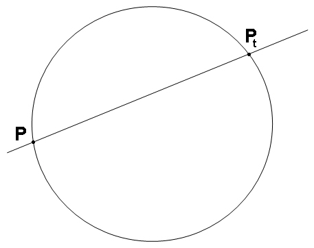
Figure 1. Parametrizing the Unit Circle

The geometric method for finding a parametrization of the rational points on the unit circle (these are points $(x,y)$ with $x,y\in{\mathbb{Q}}$ such that $x^{2}+y^{2}=1$) is the following: given a point such as $Q=(-1,0)$, the lines $y=t(x+1)$ through $Q$ intersect the circle in $Q$ and another point $P_{t}$, which is easily computed as

$$P_{t}=\bigg{(}\frac{1-t^{2}}{1+t^{2}},\frac{2t}{1+t^{2}}\bigg{)}.$$

Each rational slope gives a rational point, and conversely, every rational point $P=(x,y)\neq Q$ on the unit circle has the form $P=P_{t}$ for $t=\frac{y}{x+1}$. Thus the parametrization ${\mathbb{Q}}\longrightarrow{\mathcal{C}}\setminus\{Q\}:t\longmapsto P_{t}$ is a bijection between the affine line over ${\mathbb{Q}}$ and the conic (minus $Q$). Allowing $t=\infty$ gives a bijection between the projective line ${\mathbb{P}}^{1}{\mathbb{Q}}$ and ${\mathcal{C}}({\mathbb{Q}})$. Setting $t=\frac{m}{n}$ then provides us with the parametrization

$$x=m^{2}-n^{2},\quad y=2mn,\quad z=m^{2}+n^{2}$$

of Pythagorean triples, i.e., integral solutions of the equation $x^{2}+y^{2}=z^{2}$.

The same argument goes through for all irreducible conics: if we know a single point $P$ on a conic ${\mathcal{C}}$, we can find all of them by intersecting ${\mathcal{C}}$ with lines through $P$. Some conics, such as $x^{2}+y^{2}=3$, do not have any points over certain fields like ${\mathbb{Q}}$ or ${\mathbb{F}}_{3}$; for parametrizing them, we have to find a point over an extension field (such as ${\mathbb{Q}}(\sqrt{3}\,)$, ${\mathbb{Q}}(i)$ or ${\mathbb{F}}_{9}$), and the formulas giving the parametrization then will involve certain irrationals.

The parametrization of conics can be used for solving a variety of problems. The Arabs already knew how to find infinitely many integral solutions of the equation $x^{4}+y^{2}=z^{2}$ by solving $X^{2}+y^{2}=z^{2}$ and showing that $X=x^{2}$ infinitely often. Their unability of solving the similar equation $x^{4}+y^{4}=z^{2}$ made them conjecture that there are no integral solutions; Fermat and Euler later found full proofs.

The rational parametrization of the unit circle can be used to transform integrals of the type $\int\frac{dx}{\sqrt{1-x^{2}}}$ into integrals of rational functions. The substitution $x=\frac{t^{2}-1}{t^{2}+1}$ gives $y=\sqrt{1-x^{2}}=\frac{2t}{t^{2}+1}$ (with positive $t$ if we take the square root to be positive), hence

$$\int_{-1}^{1}\frac{dx}{\sqrt{1-x^{2}}}=2\int_{0}^{\infty}\frac{dt}{t^{2}+1}.$$

Euler also showed how to use the parametrization of conics in solving $y^{2}=x^{3}+1$: shifting the equation by $x=z-1$ give $y^{2}=z(z^{2}-3z+3)$; the factors on the right have greatest common divisor $\gcd(z,z^{2}-3z+3)=\gcd(z,3)$, hence are coprime or have gcd $3$. Unique factorization implies that the factors are either squares or three times squares (up to sign). The case $z=r^{2}$ leads, for example, to the quartic curve $y^{2}=r^{4}-3r^{2}+3$. By studying these quartics arising from $y^{2}=x^{3}+1$ Euler found all rational points on this elliptic curve (see [11] for an exposition of Euler’s proof).

More generally, solving equations such as $y^{2}=x(x^{2}+ax+b)$ over the rationals (that is, finding rational points on the elliptic curve $E:y^{2}=x(x^{2}+ax+b)$ with discriminant $\Delta=16b^{2}(a^{2}-4b)$ and its dual curve $E^{\prime}:y^{2}=x(x^{2}+a^{\prime}x+b^{\prime})$ with $a^{\prime}=-2a$ and $b^{\prime}=a^{2}-4b$) inevitably leads to the problem of deciding whether the finitely many equations

(1) $$b_{1}m^{4}+am^{2}n^{2}+b_{2}n^{4}=e^{2},$$

where $b_{1}b_{2}=b$, have nontrivial solutions in the rationals. A necessary condition for solvability in the rationals is solvability in all completions of the rationals. This condition can be checked in finitely many steps thanks to the following result, which can also be proved using the parametrization of conics (see [1]):

Proposition 1.

The equation $b_{1}m^{4}+am^{2}n^{2}+b_{2}n^{4}=e^{2}$ has nontrivial solutions in the $p$-adic integers ${\mathbb{Z}}_{p}$ for all primes $p\nmid 2ab_{1}b_{2}(a^{2}-4b_{1}b_{2})$.

This means that for checking the solvability of $b_{1}m^{4}+am^{2}n^{2}+b_{2}n^{4}=e^{2}$ in all completions of ${\mathbb{Q}}$, we only have to look at ${\mathbb{R}}={\mathbb{Q}}_{\infty}$ and the finitely many $p$-adic fields ${\mathbb{Q}}_{p}$ for primes $p\mid 2ab_{1}b_{2}(a^{2}-4b_{1}b_{2})$.

The idea behind the proof is quite simple: first show that the conic $b_{1}x^{2}+axy+b_{2}y^{2}=z^{2}$ has a nontrivial solution in ${\mathbb{F}}_{p}$; using this point, parametrize the conic to find all of them, and then show that there is a solution $(x,y)$ for which $x=m^{2}$ and $y=n^{2}$ are both squares.

Of course the line of proof could be simplified drastically if we were able to simply write down a parametrization of (1). But there are two obstructions: for parametrizing a curve, we need a rational point to start with (whose existence we would like to prove in the first place). And even if we had such a rational point we would not be able to find such a parametrization: as we will see below, curves such as (1) cannot be parametrized.

4. Parametrizing Curves of Higher Degree.

Conics are not the only curves that can be parametrized. In fact, we can start with any ”parametrization”, say

$$x=\frac{t(t^{2}+1)}{t^{4}+1},\quad y=\frac{t(t^{2}-1)}{t^{4}+1}$$

and then find the equation of the corresponding plane algebraic curve by eliminating $t$ from these equations.

The cubics with a singularity at the origin have the form $y^{2}=x^{3}+ax^{2}$; the cubic $y^{2}=x^{3}+x^{2}$, for example, has a singular point at the origin $O$, and using lines through $O$ we find the parametrization $x=t^{2}-1$, $y=t^{3}-t$.

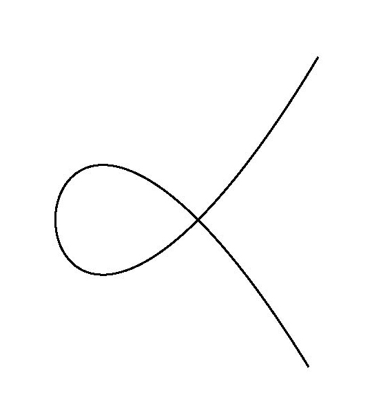
Figure 2. The singular cubic $y^{2}=x^{3}+x^{2}$

Just as the parametrization of conics has applications to calculus, so does the parametrization of cubics. For example, this technique allows us to compute the area of the region enclosed by the curve $y^{2}=x^{3}+x^{2}$: we have

$$A=2\int_{-1}^{0}y\,dx=\int_{0}^{1}2t(t-t^{3})\,dt=\frac{8}{15}.$$

Absilutely irreducible Curves with degree $n$ having a singularity of multiplicity $n-1$ can be parametrized by using a pencil of lines through the singularity. In fact, assume that the curve ${\mathcal{C}}:F(X,Y)=0$ is defined by an equation $F(X,Y)=F_{n}(X,Y)+F_{n-1}(X,Y)$, where $F_{m}$ denotes a polynomial in which each term has degree $m$ (for example, $F(X,Y)=X^{4}-X^{2}Y^{2}+Y^{3}$ can be written as $F(X,Y)=F_{4}(X,Y)+F_{3}(X,Y)$ with $F_{4}(X,Y)=X^{4}-X^{2}Y^{2}$ and $F_{3}(X,Y)=Y^{3}$). Plugging the line equation $Y=tX$ into $F(X,Y)=0$ gives

$$0=F_{n}(X,tX)+F_{n-1}(X,tX)=X^{n}F_{n}(1,t)+X^{n-1}F_{n-1}(1,t).$$

The solution $X=0$ gives the singular point; the nonzero solution gives the following well-known parametrization:

Proposition 2.

Let the curve ${\mathcal{C}}:F(X,Y)=0$ be defined by a polynomial $F(X,Y)=F_{n}(X,Y)+F_{n-1}(X,Y)$, where $F_{m}$ denotes a polynomial in which each term has degree $m$; then

$$X=-\frac{F_{n-1}(1,t)}{F_{n}(1,t)},\qquad Y=-t\cdot\frac{F_{n-1}(1,t)}{F_{n}(1,t)}$$

is a parametrization of ${\mathcal{C}}$.

Finding a parametrization of the lemniscate $(X^{2}+Y^{2})^{2}=X^{2}-Y^{2}$ is more difficult. It is a straightforward exercise to compute the singular points of the lemniscate: it has three double points, one at the origin $[0:0:1]$ and two conjugate singular points $[1:\pm i:0]$ at infinity. Each of the points $[1:\pm i:0]$ lies on the projective closure of the circle $(x-a)^{2}+(y-b)^{2}=c$. The circles going through the origin $O$ whose tangent in $O$ is $Y=X$ have equation $X^{2}+Y^{2}+tX-tY=0$.

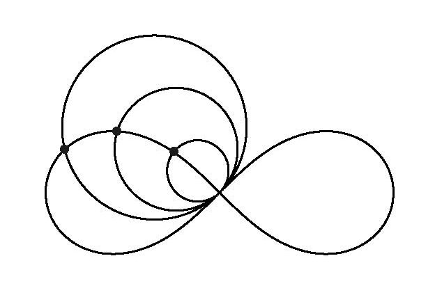
Figure 3. The lemniscate and three circles ($t=0.25$, $0.5$, $0.75$)

These circles intersect the lemniscate with multiplicity $2$ in $[1:\pm i:0]$ and with multiplicity $\geq 3$ in $O$, and since there are exactly $8=2\cdot 4$ points of intersection by Bezout’s Theorem, the circles will intersect the lemniscate in exactly one other point, whose coordinates will be rational if $t$ is rational. Thus we can parametrize the lemniscate using the pencil $X^{2}+Y^{2}+tX-tY=0$ of circles. Here are the calculations (we use affine coordinates): substitute $X^{2}+Y^{2}=t(Y-X)$ in the equation of the lemniscate; this gives

$$0=t^{2}(X-Y)^{2}-(X^{2}-Y^{2})=(X-Y)[t^{2}(X-Y)-(X+Y)]=0.$$

The first factor leads to the known point $O$; setting the second factor equal to $0$ yields $X(t^{2}-1)=Y(t^{2}+1)$. Solving for $Y$ and plugging this into the equation of the circle gives a quadratic equation in $X$ without constant term; the nonzero solution gives the parametrization of the lemniscate:

Proposition 3.

The lemniscate $(X^{2}+Y^{2})^{2}=X^{2}-Y^{2}$ admits the parametrization

$$X(t)=\frac{t(t^{2}+1)}{t^{4}+1},\quad Y(t)=\frac{t(t^{2}-1)}{t^{4}+1}.$$

In fact, any irreducible quartic $F(X,Y,Z)=0$ with three double points can be parametrized (see [16]): move the singular points to $[0:0:1]$, $[0:1:0]$ and $[1:0:0]$ by a suitable projective transformation; the fact that these points are singular implies that $F$ has the form

$$F(X,Y,Z)=aX^{2}Y^{2}+bY^{2}Z^{2}+cX^{2}Z^{2}+dXYZ^{2}+eYZX^{2}+fXZY^{2}.$$

Applying the quadratic transformation

$$X=\frac{1}{x},\quad Y=\frac{1}{y},\quad Z=\frac{1}{z}$$

and clearing denominators we end up with a conic, which can easily be parametrized by rational functions.

5. Curves without Parametrization

After having given lots of examples for parametrized families of rational solutions of certain diophantine equations we now turn to the problem of showing that certain curves cannot be parametrized by rational functions. An effective tool for doing so is provided by the theorem of Stothers-Mason.

For fields $K$, the polynomial ring $K[T]$ is Euclidean and therefore a unique factorization domain; thus every nonzero polynomial $A\in K[T]$ can be written uniquely as a product $A=p_{1}(T)^{a_{1}}\cdots p_{r}(T)^{a_{r}}$ of prime powers. We define the radical ${\operatorname{rad}\,}A$ of $A$ as the product ${\operatorname{rad}\,}A=p_{1}(T)\cdots p_{r}(T)$.

Theorem 2 (Stothers-Mason).

Let $K$ be a field of characteristic $0$. If $A,B,C$ are nonzero polynomials in $K[T]$ with $A+B+C=0$ and $\gcd(A,B,C)=1$, then

(2) $$\max\{\deg A,\deg B,\deg C\}\leq\deg{\operatorname{rad}\,}ABC-1.$$

As a corollary, we find that the curve $x^{n}+y^{n}=1$ cannot be parametrized for exponents $n>2$, which is called Fermat’s Last Theorem for polynomials:

Corollary 1.

The Fermat curve $x^{n}+y^{n}=1$ does not have a nontrivial ${\mathbb{C}}(t)$-rational point for $n>2$.

Proof.

Assume that the Fermat curve admits a rational parametrization by nonconstant polynomials with coefficients in ${\mathbb{C}}$. Clearing denominators we find polynomials $x,y,z\in K[T]$ with $x(T)^{n}+y(T)^{n}-z(T)^{n}=0$, which we may assume to be pairwise coprime. By Mason’s Theorem, we have

$$\deg x(T)^{n}\leq\deg{\operatorname{rad}\,}(xyz)-1=s-1,$$

where $s$ is the number of distinct roots of $xyz$. Thus $s\leq\deg xyz$, and therefore

$$n\deg x=\deg x^{n}\leq\deg x+\deg y+\deg z-1.$$

The same inequality holds for $y$ and $z$; adding them gives

$$n(\deg x+\deg y+\deg z)\leq 3(\deg x+\deg y+\deg z)-3,$$

which implies that $n<3$. ∎

Although Fermat’s Last Theorem for polynomials follows quite easily, from Mason’s Theorem, it is not clear how to apply it to general algebraic curves. On the other hand it is possible to derive quite strong conditions on e.g. the solvability of polynomial Pell equations: Consider the equation $X^{2}-DY^{2}=1$, where $D\in{\mathbb{C}}[T]$ is a nonconstant polynomial of degree $\deg D>0$. Let $n(D)$ denote the number of distinct zeros of $D$. Then we claim

Proposition 4.

Let $D\in{\mathbb{C}}[T]$ be a polynomial. If the equation $X^{2}-DY^{2}=1$ has a nontrivial solution (i.e. with $Y\neq 0$), then $\deg D\leq 2n(D)-2$.

Proof.

Applying Thm. 2 to $X^{2}-DY^{2}-1=0$ we get

$$2\deg X =\deg X^{2}\leq\deg X+\deg Y+n(D)-1,$$

$$2\deg Y+\deg D =\deg DY^{2}\leq\deg X+\deg Y+n(D)-1.$$

Adding these inequalities shows that if $X^{2}-DY^{2}-1=0$ has a nonzero solution, then $\deg D\leq 2n(D)-2$. Conversely, if $\deg D\geq 2n(D)-1$, the equation has no nonzero solution. ∎

6. Kapferer’s Proof

We have already seen that irreducible conics with a rational point can always be parametrized. For irreducible cubics, the situation is also clear: if ${\mathcal{C}}$ is a singular irreducible cubic, then it has a unique singular point $P$, and by intersecting the lines through $P$ with ${\mathcal{C}}$ it is then easy to find a parametrization. Smooth cubics, on the other hand, cannot be parametrized by rational functions, as we will see below. For quartics ${\mathcal{C}}$, there are already a lot of cases: an irreducible quartic can have at most three singular points (if there are four of them, pick a fifth point on the quartic; the conic through these five points then intersects the quartic with multiplicity $\geq 9$, which implies by Bezout’s Theorem that the conic is a component of the quartic); if ${\mathcal{C}}$ has three double points, then it can be parametrized by looking at the family of conics going through the three singular points and some fixed smooth point on the quartic; each such conic intersects the quartic in exactly one other point, which gives the required parametrization.

Clebsch showed that the genus of a plane algebraic curve can be computed as follows: using birational transformations (the genus is a birational invariant), transform the curve into a curve whose only singularities are simple nodes or cusps. If ${\mathcal{C}}$ is an irreducible plane algebraic curve with at most double points as singularities, and if $d$ denotes the degree of ${\mathcal{C}}$ and $r$ the number of double points, then

$$g=\frac{(d-1)(d-2)}{2}-r$$

is called the genus of ${\mathcal{C}}$.

Clebsch [3] then proved that a plane algebraic curve can be parametrized by rational functions if and only if its genus is $0$; he also showed in [4] that curves of genus $1$ can be parametrized by elliptic functions. Kapferer [9] observed that the following special case of Clebsch’s theorem on the rational parametrization of curves can be proved quite easily:

Theorem 3.

Let $K$ be a field with characteristic $0$. Let ${\mathcal{C}}$ be a nonsingular curve defined by the homogeneous polynomial $F(X,Y,Z)\in K[X,Y,Z]$ of degree $n\geq 1$. If ${\mathcal{C}}$ can be parametrized, that is, if there exist nonconstant coprime homogeneous polynomials $f,g,h\in K[U,V]$ of degree $m\geq 1$ such that $F(f,g,h)=0$ identically, then $n\leq 2$.

In particular, elliptic curves (smooth cubic curves with at least one rational point) cannot be parametrized with rational functions.

Proof.

Assume that there is a parametrization $F(f,g,h)=0$ as described in the statement of the Theorem. Taking the derivatives of this equation with respect to $U$ and $V$ we find

$$F_{X}(f,g,h)f_{U}+F_{Y}(f,g,h)g_{U}+F_{Z}(f,g,h)h_{U} =0,$$

$$F_{X}(f,g,h)f_{V}+F_{Y}(f,g,h)g_{V}+F_{Z}(f,g,h)h_{V} =0.$$

These equations can be written in matrix form

(3) $$\bigg{(}\begin{matrix}f_{U}&g_{U}&h_{U}\\ f_{V}&g_{V}&h_{V}\end{matrix}\bigg{)}\left(\begin{matrix}F_{X}(f,g,h)\\ F_{Y}(f,g,h)\\ F_{Z}(f,g,h)\end{matrix}\right)=0.$$

We now start with two little lemmas:

Lemma 1.

The $2\times 3$-matrix in (3) has rank $2$.

If not, then its three columns are linearly dependent, hence its three minors vanish. But $f_{U}g_{V}-f_{V}g_{U}=0$, together with Euler’s identities

$$mf=Uf_{U}+Vf_{V},\qquad mg=Ug_{U}+Vg_{V},$$

implies $U(f_{U}g_{V}-f_{V}g_{U})=m(f\cdot g_{V}-g\cdot f_{V})=0$, hence $f\cdot g_{V}-g\cdot f_{V}=0$. Since $f$ and $g$ were assumed to be coprime, this implies $f\mid f_{V}$ and hence $f_{V}=0$ (the same argument, by the way, occurs in Snyder’s proof of Mason’s theorem). Similarly, it follows that $f_{U}=0$. Since $K$ has characteristic $0$, this is only possible if $\deg f\leq 0$, which contradicts our assumptions.

Lemma 2.

The polynomials $F_{X}(f,g,h)$, $F_{Y}(f,g,h)$ and $F_{Z}(f,g,h)$ are coprime.

In fact, assume not; then, over some algebraic closure of $K$ they will have at least a linear factor $U-cV$ in common. Setting $x=f(c,1)$, $y=g(c,1)$ and $z=h(c,1)$ we have $(x,y,z)\neq(0,0,0)$: otherwise $f,g,h$ would have a common factor $U-cV$ contrary to our assumptions. Moreover, we have $F_{X}(x,y,z)=F_{Y}(x,y,z)=F_{Z}(x,y,z)=0$, and this implies that $(x:y:z)$ is a singular point on ${\mathcal{C}}$.

Now we can complete the proof of the theorem. We now know that the solution space of the linear system of equations

(4) $$\bigg{(}\begin{matrix}f_{U}&g_{U}&h_{U}\\ f_{V}&g_{V}&h_{V}\end{matrix}\bigg{)}\left(\begin{matrix}P\\ Q\\ R\end{matrix}\right)=0$$

in the $3$-dimensional $K(U,V)$-vector space has dimension $1$. Developing the determinants of the matrices

$$M=\left(\begin{matrix}f_{U}&g_{U}&h_{U}\\ f_{U}&g_{U}&h_{U}\\ f_{V}&g_{V}&h_{V}\end{matrix}\right)\quad\text{and}\quad N=\left(\begin{matrix}f_{V}&g_{V}&h_{V}\\ f_{U}&g_{U}&h_{U}\\ f_{V}&g_{V}&h_{V}\end{matrix}\right)$$

with respect to the first line shows that $0=\det M=f_{U}P+g_{U}Q+h_{U}R$ and $0=\det N=f_{V}P+g_{V}Q+h_{V}R$, where

$$P=\bigg{|}\begin{matrix}g_{U}&h_{U}\\ g_{V}&h_{V}\end{matrix}\bigg{|},\qquad Q=-\bigg{|}\begin{matrix}f_{U}&h_{U}\\ f_{V}&h_{V}\end{matrix}\bigg{|},\qquad R=\bigg{|}\begin{matrix}f_{U}&g_{U}\\ f_{V}&g_{V}\end{matrix}\bigg{|}.$$

This provides us with a solution of (4). Since $P=F_{X}(f,g,h)$, $Q=F_{Y}(f,g,h)$ and $R=F_{Z}(f,g,h)$ is another solution, the fact that the solution space has dimension $1$ implies that these solutions are linearly dependent over $K(U,V)$. Thus there exists a rational function $\frac{p(U,V)}{q(U,V)}$ with coprime polynomials $p,q\in K[U,V]$ such that

$$q(U,V)(h_{U}g_{V}-h_{V}g_{U}) =p(U,V)F_{X}(f,g,h),$$

$$q(U,V)(f_{U}h_{V}-f_{V}h_{U}) =p(U,V)F_{Y}(f,g,h),$$

$$q(U,V)(g_{U}f_{V}-g_{V}f_{U}) =p(U,V)F_{Z}(f,g,h).$$

These equations imply that $q(U,V)=q$ is a constant: in fact, each irreducible factor of $q$ must divide $F_{X}(f,g,h)$, $F_{Y}(f,g,h)$, and $F_{Z}(f,g,h)$, hence their gcd, which is trivial by our second claim.

Next we compute degrees; on the left hand side we get

$$\deg q(h_{U}g_{V}-h_{V}g_{U})=\deg(h_{U}g_{V}-h_{V}g_{U})\leq\deg h_{U}g_{V}=2(m-1).$$

On the right hand side, we find

$$\deg p\cdot F_{X}(f,g,h)\geq\deg F_{X}(f,g,h)=(n-1)m.$$

Comparing degrees now shows that $2m-2\geq m(n-1)$, which implies $-2\geq m(n-3)$ and therefore $n<3$. ∎

This is not the best possible result that can be achieved by this line of attack. It is easy to prove that irreducible curves with a single double point cannot be parametrized by rational functions whenever the curve has degree $\geq 4$. Gradually generalizing this proof will ultimately lead to a proof of Clebsch’s result that a curve cannot be parametrized if its genus is positive.

References

- [1] W. Aitken, F. Lemmermeyer, Counterexamples to the Hasse principle: an elementary introduction, Amer. Math. Monthly (2011), to appear
- [2] A. Clebsch, Über einen Satz von Steiner und einige Punkte der Theorie der Curven dritter Ordnung, J. Reine Angew. Math. 63 (1863), 94–121
- [3] A. Clebsch, Über diejenigen ebenen Kurven, deren Koordinaten rationale Funktionen eines Parameters sind, J. Reine Angew. Math. 64 (1865), 43–65
- [4] A. Clebsch, Über diejenigen Kurven, deren Koordinaten sich als elliptische Funktionen eines Parameters darstellen lassen, J. Reine Angew. Math. 64 (1865), 210–270
- [5] A. Clebsch, Vorlesungen über die Geometrie, lecture notes 1871/72, Lindemann (ed.)
- [6] W. Fulton, Algebraic Curves, New York - Amsterdam, Benjamin 1969
- [7] D. Hilbert, A. Hurwitz, Über die diophantischen Gleichungen vom Geschlecht Null, Acta Math. 14 (1891), 217–224
- [8] C. Juel, Ueber die Parameterbestimmung von Punkten auf Curven zweiter und dritter Ordnung. Eine geometrische Einleitung in die Theorie der logarithmischen und elliptischen Funktionen, Math. Ann. 47 (1896), 72–104
- [9] H. Kapferer, Über das Kriterium der Rationalität einer algebraischen Kurve, Sitz.-ber. München (1930), 123–128
- [10] L. Kronecker, Vorlesungen über Zahlentheorie, (K. Hensel, ed.) Teubner, Leipzig (1901); reprint Springer-Verlag (1978)
- [11] F. Lemmermeyer, A note on Pépin’s counterexamples to the Hasse principle for curves of genus 1, Abh. Math. Semin. Univ. Hamb. 69 (1999), 335–345
- [12] L.J. Mordell On the rational solutions of the indeterminate equations of the third and fourth degrees, Cambr. Phil. Soc. Proc. 21 (1922), 179–192
- [13] I. Newton, The Mathematical Papers of Isaac Newton, vol. 4, (D.T. Whiteside, ed.), Cambridge 1971
- [14] H. Poincaré, Sur les propriétés arithmétiques des courbes algébriques, J. Math. (5) 7 (1901), 161–233; Œuvres 5 (1950), 483–548
- [15] M. Reid, Undergraduate algebraic geometry, LMS Student Texts 12, CUP 1988
- [16] P. Samuel, Projective geometry, Springer-Verlag 1988
- [17] J.R. Sendra, F. Winkler, S. Pérez-Díaz, Rational Algebraic Curves - A Computer Algebra Approach, Springer-Verlag 2008
- [18] I.R. Shafarevich, Basic Algebraic Geometry. 1: Varieties in projective space, Transl. from the Russian by Miles Reid. 2nd ed. Springer-Verlag (1994)
- [19] I.R. Shafarevich, Zum 150. Geburtstag von Alfred Clebsch, Math. Ann. 266 (1869), 135–140
- [20] N. Snyder, An alternate proof of Mason’s theorem, Elem. Math. 55 (2000), 93–94