A well-balanced finite volume scheme for 1D hemodynamic simulations

Abstract

English version: We are interested in simulating blood flow in arteries with variable elasticity with a one dimensional model. We present a well-balanced finite volume scheme based on the recent developments in shallow water equations context. We thus get a mass conservative scheme which also preserves equilibria of $Q=0$. This numerical method is tested on analytical tests.

Version Française : Nous nous intéressons à la simulation d’écoulements sanguins dans des artères dont les parois sont à élasticité variable. Ceci est modélisé à l’aide d’un modèle unidimensionnel. Nous présentons un schéma ”volume fini équilibré” basé sur les développements récents effectués pour la résolution du système de Saint-Venant. Ainsi, nous obtenons un schéma qui préserve le volume de fluide ainsi que les équilibres au repos: $Q=0$. Le schéma introduit est testé sur des solutions analytiques.

Introduction

We consider the following system of mass and momentum conservation with non dimensionless parameters and variables, which is the 1D model of blood flow in an artery or a vessel with non uniform elasticity (it is rewritten in a conservative form compared to what we usually find in litterature)

$$\left\{\begin{array}[]{l}\partial_{t}A+\partial_{x}Q=0\\ \partial_{t}Q+\partial_{x}\left[\dfrac{Q^{2}}{A}+\dfrac{1}{3\sqrt{\pi}\rho}kA^{3/2}\right]=\dfrac{A}{\sqrt{\pi}\rho}\left(\partial_{x}{\cal A}_{0}-\dfrac{2}{3}\sqrt{A}\partial_{x}k\right)-C_{f}\dfrac{Q}{A}\end{array}\right.,$$ (1)

with ${\cal A}_{0}=k\sqrt{A_{0}}$ and where $A(x,t)$ is the cross-section area ($A=\pi R^{2}$ with $R$ the radius of the arteria), $Q(x,t)=A(x,t)u(x,t)$ the flow rate or the discharge, $u(t,x)$ the mean flow velocity, $\rho$ the blood density, $A_{0}(x)$ the cross section at rest and $k(x)$ the stiffness of the artery. System (1) is into the form of the Saint-Venant problem with variable pressure presented in [3]. We have to mention that arterial pulse wavelengths are long enough to justify the use of a 1D model rather than a 3D model when a global simulation of blood flow in the cardiovascular system is needed.

1 Numerical method

Since [2, 8], it is well known (in the shallow water community) that the scheme should be well-balanced for good source term treatment, i.e. the scheme should preserve at least some steady states. For system (1), we should preserve at least the ”man at eternal rest” or ”dead man equilibrium” [6] (without artifacts such as [10]), it writes

$$\left\{\begin{array}[]{l}u=0\\ \dfrac{1}{\sqrt{\pi}\rho}A^{3/2}k-\dfrac{A}{\sqrt{\pi}\rho}{\cal A}_{0}=Cst\end{array}\right.,$$ (2)

this means that steady states at rest are preserved (this is the analogous of the ”lake at rest” equilibrium). Thus we use the scheme proposed in [3, p.93-94] for that kind of model. This is a finite volume scheme with a modification of the hydrostatic reconstruction (introduced in [1, 3] for the shallow water model).

1.1 Convective step

For the homogeneous system

$$\partial_{t}U+\partial_{x}F(U,Z)=0,$$ (3)

which is (1) with:

$$U=\left(\begin{array}[]{c}A\\ Q\end{array}\right),\;Z=\left(\begin{array}[]{c}{\cal A}_{0}\\ k\end{array}\right)\;\text{and}\;F(U,k)=\left(\begin{array}[]{c}Q\\ Q^{2}/A+kA^{3/2}/(3\sqrt{\pi}\rho)\end{array}\right),$$

an explicit first order conservative scheme writes

$$\dfrac{U_{i}^{n+1}-U_{i}^{n}}{\Delta t}+\dfrac{F_{i+1/2}^{n}-F_{i-1/2}^{n}}{\Delta x}=0,$$ (4)

where $U_{i}^{n}$ is an approximation of $U$

$$U_{i}^{n}\simeq\dfrac{1}{\Delta x}\int_{x_{i-1/2}}^{x_{i+1/2}}U(x,t_{n})dx.$$

$i$ refers to the cell $C_{i}=(x_{i-1/2},x_{i+1/2})=(x_{i-1/2},x_{i-1/2}+\Delta x)$ and $n$ to time $t_{n}$ with $t_{n+1}-t_{n}=\Delta t$.
The two points numerical flux

$$F_{i+1/2}^{n}={\cal F}(U_{i}^{n},U_{i+1}^{n},k_{i+1/2}^{*}),$$

with $k_{i+1/2}^{*}=\max(k_{i},k_{i+1})$, is an approximation of the flux function $F(U,Z)$ at the cell interface $i+1/2$. This numerical flux will be detailled in subsection 1.3.

1.2 Source terms treatment

In system (1), the terms $A(\partial_{x}{\cal A}_{0}-2\sqrt{A}\partial_{x}k/3)/(\sqrt{\pi}\rho)$ are involved in steady states preservation, they need a well-balanced treatment: the variables are reconstructed locally thanks to a variant of the hydrostatic reconstruction [3, p.93-94]

$$\left\{\begin{array}[]{l}\sqrt{A_{i+1/2L}}=\max(k_{i}\sqrt{A_{i}}+\min(\Delta{{\cal A}_{0}}_{i+1/2},0),0)/k^{*}_{i+1/2}\\ U_{i+1/2L}=(A_{i+1/2L},A_{i+1/2L}.u_{i})^{t}\\ \sqrt{A_{i+1/2R}}=\max(k_{i+1}\sqrt{A_{i+1}}-\max(\Delta{{\cal A}_{0}}_{i+1/2},0),0)/k^{*}_{i+1/2}\\ U_{i+1/2R}=(A_{i+1/2R},A_{i+1/2R}.u_{i+1})^{t}\end{array}\right.,$$ (5)

with $\Delta{{\cal A}_{0}}_{i+1/2}={{\cal A}_{0}}_{i+1}-{{\cal A}_{0}}_{i}=k_{i+1}\sqrt{{A_{0}}_{i+1}}-k_{i}\sqrt{{A_{0}}_{i}}$ and $k_{i+1/2}^{*}=\max(k_{i},k_{i+1})$. For consistency, the scheme (4) is modified as follows

$$U_{i}^{n+1}=U_{i}^{n}-\dfrac{\Delta t}{\Delta x}\left(F_{i+1/2L}^{n}-F_{i+1/2R}^{n}\right),$$ (6)

where

$$\begin{array}[]{l}F_{i+1/2L}^{n}=F_{i+1/2}^{n}+S_{i+1/2L}\\ F_{i-1/2R}^{n}=F_{i-1/2}^{n}+S_{i-1/2R}\end{array},$$

with

$$\begin{array}[]{c}F_{i+1/2}^{n}={\cal F}\left(U_{i+1/2L},U_{i+1/2R},k_{i+1/2}^{*}\right)\\ S_{i+1/2L}=\left(\begin{array}[]{c}0\\ {\cal P}(A_{i}^{n},k_{i})-{\cal P}(A_{i+1/2L}^{n},k_{i+1/2}^{*})\end{array}\right)\\ S_{i-1/2R}=\left(\begin{array}[]{c}0\\ {\cal P}(A_{i}^{n},k_{i})-{\cal P}(A_{i-1/2R}^{n},k_{i-1/2}^{*})\end{array}\right)\end{array}$$

and ${\cal P}(A,k)=kA^{3/2}/(3\rho\sqrt{\pi})$. Thus the variation of the radius and the varying elasticity are treated under a well-balanced way. In system (1), the friction term $-C_{f}Q/A$ is treated semi-implicitly. This treatment is classical in shallow water simulations [4, 11] and had shown to be efficient in blood flow simulation as well [6]. This treatment does not break the ”dead man” equilibrium. It consists in using first (6) as a prediction step without friction, i.e.:

$$U_{i}^{*}=U_{i}^{n}-\dfrac{\Delta t}{\Delta x}\left(F_{i+1/2L}^{n}-F_{i-1/2R}^{n}\right),$$

then we apply a semi-implicit friction correction on the predicted values ($U_{i}^{*}$):

$$A_{i}^{*}\left(\dfrac{u_{i}^{n+1}-u_{i}^{*}}{\Delta t}\right)=-C_{f}u_{i}^{n+1}.$$

Thus we get the corrected velocity $u_{i}^{n+1}$ and we have $A_{i}^{n+1}=A_{i}^{*}$.

1.3 HLL numerical flux

As presented in [6], several numerical fluxes might be used (Rusanov, HLL, VFRoe-ncv and kinetic fluxes). In this work we will use the HLL flux (Harten Lax and van Leer [9]) because it is the best compromise between accuracy and CPU time consuming (see [5, chapter 2]). It writes:

$${\cal F}(U_{L},U_{R},k^{*})=\left\{\begin{array}[]{ll}F(U_{L},k^{*})&\text{if}\;0\leq c_{1}\\ \dfrac{c_{2}F(U_{L},k^{*})-c_{1}F(U_{R},k^{*})}{c_{2}-c_{1}}+\dfrac{c_{1}c_{2}}{c_{2}-c_{1}}(U_{R}-U_{L})&\text{if}\;c_{1}<0<c_{2}\\ F(U_{R},k^{*})&\text{if}\;c_{2}\leq 0\end{array}\right.,$$

with

$$c_{1}={\inf\limits_{U=U_{L},U_{R}}}({\inf\limits_{j\in\{1,2\}}}\lambda_{j}(U,k^{*}))\;\text{and}\;c_{2}={\sup\limits_{U=U_{L},U_{R}}}({\sup\limits_{j\in\{1,2\}}}\lambda_{j}(U,k^{*})),$$

where $\lambda_{1}(U,k^{*})$ and $\lambda_{2}(U,k^{*})$ are the eigenvalues of the system and $k^{*}=\max(k_{L},k_{R})$.

To prevent blow up of the numerical values, we impose the following CFL (Courant, Friedrichs, Levy) condition

$$\Delta t\leq n_{CFL}\dfrac{\Delta x}{\max\limits_{i}(|u_{i}|+c_{i})},$$

where $c_{i}=\sqrt{k_{i}\sqrt{A_{i}}/(2\rho\sqrt{\pi})}$ and $n_{CFL}=1$.

2 Some numerical results

2.1 ”The stented man at eternal rest”

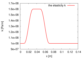
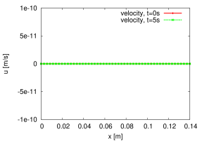
Figure 1: No spurious flows (right) are generated by a change of elasticity (left).

In this test, we consider a configuration with no flow and with a change of artery elasticity $k(x)$, this is the case for a dead man with a stented artery (see Figure 1 left). The section of the artery is constant $R_{0}(x)=4.0\;10^{-3}\text{m}$ and the velocity is $u(x,t)=0\text{m/s}$. We use the following numerical values: $J=50$ cells, $C_{f}=0$, $\rho=1060\text{m}^{3}$, $L=0.14\text{m}$, $T_{end}=5\text{s}$. As initial conditions, we take a fluid at rest $Q(x,0)=0\text{m}^{3}/\text{s}$ and

$$k(x)=\left\{\begin{array}[]{ll}k_{0}&\text{if}\;x\in[0:x_{1}]\cup[x_{4}:L]\\ k_{0}+\dfrac{\Delta k}{2}\left(\sin\left(\dfrac{x-x_{1}}{x_{2}-x_{1}}\pi-\pi/2\right)+1\right)&\text{if}\;x\in]x_{1}:x_{2}[\\ k_{0}+\Delta k&\text{if}\;x\in[x_{2}:x_{3}]\\ k_{0}+\dfrac{\Delta k}{2}\left(\cos\left(\dfrac{x-x_{3}}{x_{4}-x_{3}}\pi\right)+1\right)&\text{if}\;x\in]x_{3}:x_{4}[\end{array}\right.,$$

with $k_{0}=1.0\;10^{8}\text{Pa}/\text{m}$, $\Delta k=6.0\;10^{7}\text{Pa}/\text{m}$, $x_{1}=1.0\;10^{-2}\text{m}$, $x_{2}=3.05\;10^{-2}\text{m}$, $x_{3}=4.95\;10^{-2}\text{m}$ and $x_{4}=7.0\;10^{-2}\text{m}$.

The steady state at rest is perfectly preserved in time, we do not notice any spurious oscillation (see Figure 1 right).

2.2 Wave reflection-transmission in a stented artery

We now observe the reflexion and transmission of a pulse through a sudden change of artery elasticity (from $k_{R}$ to $k_{L}$ with $k_{L}>k_{R}$) in an elastic tube of constant radius (see Figure 2 left). We take the following numerical values: $J=1500$ cells, $C_{f}=0$, $k_{L}=1.6\;10^{8}\text{Pa/m}$, $k_{R}=1.\;10^{8}\text{Pa/m}$, $\Delta k=6.\;10^{7}\text{Pa/m}$, $\rho=1060\text{m}^{3}$, $R_{0}=4.0\;10^{-3}\text{m}$, $L=0.16\text{m}$, $T_{end}=8.0\;10^{-3}\text{s}$, $c_{L}=\sqrt{k_{L}R/(2\rho)}\simeq 17.37\text{m/s}$ and $c_{R}=\sqrt{k_{R}R/(2\rho)}\simeq 13.74\text{m/s}$. We take a decreasing elasticity on a rather small scale:

$$k(x)=\left\{\begin{array}[]{ll}k_{R}+\Delta k&\text{if}\;x\in[0:x_{1}]\\ k_{R}+\dfrac{\Delta k}{2}\left[1+\cos\left(\dfrac{x-x_{1}}{x_{2}-x_{1}}\pi\right)\right]&\text{if}\;x\in]x_{1}:x_{2}]\\ k_{R}&\text{else}\end{array}\right.,$$

with $x_{1}=19L/40$ and $x_{2}=L/2$. As initial conditions, we consider a fluid at rest $Q(x,0)=0\text{m}^{3}/\text{s}$ and the following perturbation of radius:

$$R(x,0)=\left\{\begin{array}[]{ll}R_{0}(x)\left[1+\epsilon\sin\left(\dfrac{100}{20L}\pi\left(x-\dfrac{65L}{100}\right)\right)\right]&\text{if}\;x\in[65L/100:85L/100]\\ R_{0}(x)&\text{else}\end{array}\right.,$$

with $\epsilon=1.0\;10^{-2}$. The expression for the pressure is

$$p(x,t)=p_{0}(x)+k(x)(R(x,t)-R_{0}(x)),$$

where $p_{0}$ is the external pressure.

The numerical results perfectly match with the predictions for a linearized flow. We get the predicted amplitudes both for the transmitted and the reflected waves (see Figure 2 right).

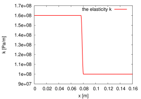
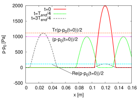
Figure 2: Across a discontinuity of $k$ (left), an initial pulse evolves (right) ; it is transmitted and reflected.

2.3 Wave ”damping”

In this case, the elasticity is constant in space. We consider the viscous term in the linearized momentum equation. A periodic signal is imposed at inflow as a perturbation of a steady state ($R_{0}=Cst$, $u_{0}=0$) with a constant section at rest. We take $R=R_{0}+\epsilon R_{1}$ and $u=0+\epsilon u_{1}$, where ($R_{1}$,$u_{1}$) is the perturbation of the steady state. Looking for progressive waves (i.e. under the form $e^{i(\omega t-Kx)}$), we take for the imposed incoming discharge

$$Q_{b}(t)=Q(t,x=0)=Q_{amp}\sin(\omega t)\;\text{m}^{3}/\text{s}.$$

Thus, we have a damping wave in the domain

$$Q(t,x)=\left\{\begin{array}[]{ll}0&\text{if}\;k_{r}x>\omega t\\ Q_{amp}\sin(\omega t-k_{r}x)e^{k_{i}x}&\text{if}\;k_{r}x\leq\omega t\end{array}\right.,$$

with $\omega=2\pi/T_{pulse}$, $T_{pulse}$ the time length of a pulse and $K=k_{r}+ik_{i}$ the wave vector.

We use the following numerical values: $J=750$ cells, $\rho=1060\text{m}^{3}$, $L=3\text{m}$, $k=1.10^{8}\text{Pa/m}$, $R_{0}=4.10^{-3}\text{m}$ and $T_{end}=5\text{s}$. We consider both $C_{f}=0$ and $C_{f}=0.005053$. As initial conditions, we take a fluid at rest $Q(x,0)=0\text{m}^{3}/\text{s}$ and as input boundary condition

$$Q_{b}(t)=Q_{amp}\sin(\omega t),$$

with $\omega=2\pi/T_{pulse}=2\pi/0.5\text{s}$ and $Q_{amp}=3.45\;10^{-7}\text{m}^{3}/\text{s}$. The output is an outgoing wave.

The results are closed to the analytical solution (see Figure 3). We notice a small numerical diffusion for $C_{f}=0.005053$.

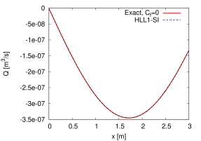
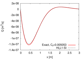
Figure 3: Response to an oscillating input condition, left with no viscosity and right with viscosity.

3 Conclusion

In this work, we have considered the 1D model of flow in an artery with varying elasticity and constant section. We have presented a well-balanced finite volume scheme. Thus we get a mass conservative scheme. Moreover, the well-balanced property allows to have a good treatment of the source, i.e. we do not get numerical artifacts. This numerical method gave good results on numerical tests. In future works, we will have to add some extra source terms in order to get a more realistic model. These extra terms will require to develop a low diffusive high order scheme in the spirit of [7]. Moreover, this will improve the accuracy of the scheme. And we will also have to test more complex cases such as bifurcations and networks.

References

• [1] E. Audusse, F. Bouchut, M.-O. Bristeau, R. Klein, and B. Perthame. A fast and stable well-balanced scheme with hydrostatic reconstruction for shallow water flows. SIAM J. Sci. Comput., 25(6):2050–2065, 2004.
• [2] Alfredo Bermudez and M. Elena Vazquez. Upwind methods for hyperbolic conservation laws with source terms. Computers & Fluids, 23(8):1049 – 1071, 1994.
• [3] F. Bouchut. Nonlinear stability of finite volume methods for hyperbolic conservation laws, and well-balanced schemes for sources, volume 2/2004. Birkhäuser Basel, 2004.
• [4] M.-O. Bristeau and Benoît Coussin. Boundary conditions for the shallow water equations solved by kinetic schemes. Technical Report 4282, INRIA, October 2001.
• [5] Olivier Delestre. Simulation du ruissellement d’eau de pluie sur des surfaces agricoles/ rain water overland flow on agricultural fields simulation. PhD thesis, Université d’Orléans (in French), available from TEL: tel.archives-ouvertes.fr/INSMI/tel-00531377/fr, July 2010.
• [6] Olivier Delestre and Pierre-Yves Lagrée. A ”well balanced” finite volume scheme for blood flow simulation. submitted.
• [7] Olivier Delestre and Fabien Marche. A numerical scheme for a viscous shallow water model with friction. J. Sci. Comput., DOI 10.1007/s10915-010-9393-y, 2010.
• [8] J. M. Greenberg and A.-Y. LeRoux. A well-balanced scheme for the numerical processing of source terms in hyperbolic equation. SIAM Journal on Numerical Analysis, 33:1–16, 1996.
• [9] Amiram Harten, Peter D. Lax, and Bram van Leer. On upstream differencing and godunov-type schemes for hyperbolic conservation laws. SIAM Review, 25(1):35–61, January 1983.
• [10] Robert Kirkman, Tony Moore, and Charlie Adlard. The Walking Dead. Image Comics, 2003.
• [11] Qiuhua Liang and Fabien Marche. Numerical resolution of well-balanced shallow water equations with complex source terms. Advances in Water Resources, 32(6):873 – 884, 2009.