Inertial-range behaviour of a passive scalar field in a random shear flow: Renormalization group analysis of a simple model

Abstract

Infrared asymptotic behaviour of a scalar field, passively advected by a random shear flow, is studied by means of the field theoretic renormalization group and the operator product expansion. The advecting velocity is Gaussian, white in time, with correlation function of the form $\propto\delta(t-t^{\prime})/k_{\bot}^{d-1+\xi}$, where $k_{\bot}=|{\bf k}_{\bot}|$ and ${\bf k}_{\bot}$ is the component of the wave vector, perpendicular to the distinguished direction (‘direction of the flow’) — the $d$-dimensional generalization of the ensemble introduced by Avellaneda and Majda [Commun. Math. Phys. 131: 381 (1990)]. The structure functions of the scalar field in the infrared range exhibit scaling behaviour with exactly known critical dimensions. It is strongly anisotropic in the sense that the dimensions related to the directions parallel and perpendicular to the flow are essentially different. In contrast to the isotropic Kraichnan’s rapid-change model, the structure functions show no anomalous (multi)scaling and have finite limits when the integral turbulence scale tends to infinity. On the contrary, the dependence of the internal scale (or diffusivity coefficient) persists in the infrared range. Generalization to the velocity field with a finite correlation time is also obtained. Depending on the relation between the exponents in the energy spectrum ${\cal E}\propto k_{\bot}^{1-\varepsilon}$ and in the dispersion law $\omega\propto k_{\bot}^{2-\eta}$, the infrared behaviour of the model is given by the limits of vanishing or infinite correlation time, with the crossover at the ray $\eta=0$, $\varepsilon>0$ in the $\varepsilon$–$\eta$ plane. The physical (Kolmogorov) point $\varepsilon=8/3$, $\eta=4/3$ lies inside the domain of stability of the rapid-change regime; there is no crossover line going through this point.

Key words: renormalization group, turbulent transport, anomalous scaling.

1 Introduction

The problem of turbulent advection, being of practical importance in itself, has become a cornerstone in studying fully developed hydrodynamical turbulence on the whole [1]. On one hand, deviations from the classical Kolmogorov theory — intermittency and anomalous scaling [2, 3] — are much stronger pronounced for a passively advected scalar field (temperature of the fluid or concentration of impurity) than for the advecting turbulent field itself. On the other, the problem of passive advection appears easier tractable theoretically. Most remarkable progress was achieved for Kraichnan’s rapid-change model: for the first time, the anomalous exponents were derived on the basis of a dynamical model and within controlled approximations [4, 5].

In Kraichnan’s model, the turbulent velocity field is modelled by the Gaussian distribution with the pair correlation function of the form

$$\langle v_{i}v_{j}\rangle\propto D_{0}\,\delta(t-t^{\prime})\,P_{ij}\,k^{-d-\xi},$$ (1.1)

where $P_{ij}=\delta_{ij}-k_{i}k_{j}/k^{2}$ is the transverse projector, $k\equiv|{\bf k}|$ is the wave number, $D_{0}>0$ is an amplitude factor, $d$ is the dimension of the ${\bf x}$ space and $\xi$ is an arbitrary exponent. The latter can be viewed as a kind of Hölder’s exponent, which measures ‘roughness’ of the velocity field; the ‘Batchelor limit’ $\xi\to 2$ corresponds to smooth velocity, while the most realistic (Kolmogorov) value is $\xi=4/3$ [1].

The issue of interest is, in particular, the behaviour of the equal-time structure functions

$$S_{n}(r)=\langle\left[\,\theta(t,{\bf x})-\theta(t,{\bf x}^{\prime})\,\right]^{n}\rangle,\quad r=|{\bf x}-{\bf x}^{\prime}|$$ (1.2)

of the scalar field $\theta(t,{\bf x})$ in the inertial range $\ell\ll r\ll{\cal L}$, where $\ell$ is the dissipation length and ${\cal L}$ is the integral turbulence scale. Within the so-called zero-mode approach, developed in [4, 5], it was shown that in the inertial range the functions (1.2) are independent of the diffusivity coefficient and have the forms:

$$S_{2n}(r)\propto D_{0}^{-n}r^{n(2-\xi)}\,(r/{\cal L})^{\Delta_{n}},$$ (1.3)

with negative anomalous exponents $\Delta_{n}$, whose first terms of the expansions in $1/d$ [4] and $\xi$ [5] are the following:

$$\Delta_{n}=-2n(n-1)\xi/d+O(1/d^{2})=-2n(n-1)\xi/(d+2)+O(\xi^{2}).$$ (1.4)

Thus the functions (1.2) depend on the integral scale and diverge for ${\cal L}\to\infty$, in contradiction with the classical Kolmogorov theory.

In [6] and subsequent papers, the field theoretic renormalization group (RG) and operator product expansion (OPE) were applied to Kraichnan’s model; see [7] for the review and references. In the RG approach, the exponent $\xi$ plays the part analogous to that played by $\varepsilon=4-d$ in Wilson’s theory of critical phenomena, while $d$ remains a free parameter. The anomalous scaling for the structure functions emerges as a consequence of the existence in the corresponding operator product expansions of ‘dangerous’ composite fields (composite operators in the field theoretic terminology) of the form $(\partial\theta)^{2n}$, whose negative critical dimensions are identified with the anomalous exponents $\Delta_{n}$. This allows one to construct a systematic perturbation expansion for the anomalous exponents and to calculate them up to the orders $\xi^{2}$ [6] and $\xi^{3}$ [8].

In this paper, the RG+OPE approach is applied to the model of a passive scalar field in a random shear flow: the Gaussian velocity field is oriented along a fixed direction ${\bf n}$ (‘direction of the flow’) and depends only on the coordinates in the subspace orthogonal to ${\bf n}$. In the momentum space, its correlation function has the form simillar to (1.1): $\langle vv\rangle\propto\delta(t-t^{\prime})\,k_{\bot}^{-d+1-\xi}$, where $k_{\bot}=|{\bf k}_{\bot}|$ and ${\bf k}_{\bot}$ is the component of the momentum ${\bf k}$ perpendicular to ${\bf n}$. This model can be viewed as a $d$-dimensional generalization of the strongly anisotropic velocity ensemble introduced in [9] in connection with the turbulent diffusion problem and further studied and generalized in a number of papers [10]–[19].

We show that the inertial-range behaviour of this model appears essentially different from the isotropic Kraichnan’s model: due to the absence of dangerous composite operators, the structure functions (1.2) have finite limits at ${\cal L}\to\infty$ and thus show no anomalous scaling in the sense of (1.3). On the contrary, dependence on the diffusivity (and thus on the dissipation length) persists in the inertial range. Following the nomenclature of the monographs [2, 3], one can say that, in complete contradistinction with isotropic Kraichnan’s model, the first Kolmogorov hypothesis is valid in the present case, while the second hypothesis is violated.

The paper is organized as follows. The sections 2–8 are devoted to the rapid-change version of the model (vanishing correlation time); generalization to the finite-correlated case is given in section 9.

In section 2 we give detailed description of the model, present its field theoretic formulation and the corresponding diagrammatic technique. In section 3 we analyze canonical dimensions and ultraviolet (UV) divergences of the model. We show that, after an appropriate extension, the model becomes multiplicatively renormalizable. We derive the explicit expression for the only independent renormalization constant, which is given exactly by the one-loop approximation. In section 4 we derive the differential RG equations with exactly known coefficients ($\beta$ function and anomalous dimensions $\gamma$) and show that they possess an infrared (IR) attractive fixed point, which governs the scaling behaviour of the Green functions in the IR range.

In section 5 we present the corresponding critical dimensions for the basic fields and parameters. Our model is strongly anisotropic in the sense that, in contrast to previous RG+OPE studies of anisotropic passive advection [20]–[22], it does not include parameters that could be tuned to make the velocity statistics isotropic, and hence it does not include the isotropic Kraichnan’s model as a special case. As an interesting consequence, the critical dimensions related to the directions parallel and perpendicular to the flow are essentially different.

Section 6 is devoted to the composite operators. As already mentioned, the key role in the RG+OPE approach to anomalous scaling is played by the dimensions of the Galilean invariant operators $(\partial\theta)^{2n}$, built of the scalar gradients [6]–[8]. In the isotropic case, there is only one such operator for a given $n$, namely $(\partial_{i}\theta\partial_{i}\theta)^{n}$. In the strongly anisotropic case of a shear flow, there is a set of $(n+1)$ relevant operators for each $n$. They mix heavily in renormalization and give rise to a set of critical dimensions rather than a single $\Delta_{n}$. Nevertheless, it turns out that exact expressions can be derived for these dimensions in our model. Furthermore, in contrast to their counterparts (1.4) in the isotropic Kraichnan’s model, they all are positive.

Sections 7 and 8 apply the results of the preceding analysis to the inertial-range asymptotic behaviour of the structure functions (1.2). In section 7 their behaviour in the IR range $r\gg\ell$ is established; it turns out that those functions retain the dependence on the UV scale $\ell$. The inertial range corresponds to the additional condition that $r\ll{\cal L}$; it is studied by means of the OPE in section 8. Due to the absence of relevant dangerous operators with negative dimensions, the structure functions appear finite for $(r/{\cal L})\to 0$ and thus show no anomalous scaling in the sense of (1.3). The resulting inertial-range asymptotic expressions, presenting the main outcome of this study, are summarized in (8.3)–(8.5).

In section 9, the generalization of the above results to the velocity ensemble with finite correlation time is given. The energy spectrum is taken in the form ${\cal E}\propto k_{\bot}^{1-\varepsilon}$, while the dispersion law is $\omega\propto k_{\bot}^{2-\eta}$. It is shown that the IR behaviour of the model is nearly exhausted by the two limiting cases: the rapid-change type behaviour, realized for $\varepsilon>\eta>0$ (with $\xi=\varepsilon-\eta>0$), and the frozen (time-independent) behaviour, realized for $\varepsilon>0$, $\eta<0$. The crossover line between the two regimes is the ray $\eta=0$, $\varepsilon>0$ in the $\varepsilon$–$\eta$ plane. In contrast to the isotropic case, where the physical (Kolmogorov) point $\varepsilon=8/3$, $\eta=4/3$ lies exactly on the crossover line between the rapid-change and frozen regimes [23]–[26], now this point lies deep inside the domain of stability of the nontrivial rapid-change behaviour; there is no crossover line going through this point. This result is in agreement with the findings of the exact analysis of the $d=(1+1)$-dimensional case by [18, 19] and in disagreement with [9]–[11]; this issue is further discussed in section 10, which is also reserved for conclusions.

2 Description of the model and the field theoretic formulation

The advection-diffusion equation for the scalar field $\theta(x)$ with $x=\{t,{\bf x}\}$ has the form

$$\nabla_{t}\theta=\nu_{0}\partial^{2}\theta+\zeta,$$ (2.1)

where

$$\nabla_{t}=\partial_{t}+v_{i}\partial_{i}$$ (2.2)

is the Galilean covariant (Lagrangian) derivative, $\partial_{t}=\partial/\partial t$, $\partial_{i}=\partial/\partial x_{i}$, $\partial^{2}=\partial_{i}\partial_{i}$ is the Laplacian, $\nu_{0}$ is the diffusion coefficient and $\zeta(t,{\bf x})$ is a Gaussian random noise with zero mean and the pair correlation function

$$\langle\zeta(t,{\bf x})\zeta(t^{\prime},{\bf x}^{\prime})\rangle=\delta(t-t^{\prime})\,C({\bf r}),\quad{\bf r}={\bf x}-{\bf x}^{\prime}.$$ (2.3)

The function $C({\bf r})$ is finite at ${\bf r}=0$ (and we assume the normalization $C(0)=1$) and rapidly decays for ${\bf r}\to\infty$; its precise form is inessential. For incompressible fluid, the velocity field ${\bf v}=\{v_{i}(x)\}$ is transverse due to the continuity relation: $\partial_{i}v_{i}=0$.

Let ${\bf n}$ be a unit constant vector that determines some distinguished direction (‘direction of the flow’). Then any vector can be decomposed into the components perpendicular and parallel to the flow, for example, ${\bf x}={\bf x}_{\bot}+{\bf n}\,x_{\parallel}$ with ${\bf x}_{\bot}\cdot{\bf n}=0$. The velocity field will be taken in the form

$${\bf v}={\bf n}v(t,{\bf x}_{\bot}),$$ (2.4)

where $v(t,{\bf x}_{\bot})$ is a scalar function independent of $x_{\parallel}$. Then the incompressibility condition is automatically satisfied:

$$\partial_{i}v_{i}=\partial_{\parallel}v(t,{\bf x}_{\bot})=0.$$ (2.5)

For $v(t,{\bf x}_{\bot})$ we assume a Gaussian distribution with zero mean and the pair correlation function of the form:

$$\langle v(t,{\bf x}_{\bot})v(t^{\prime},{\bf x}_{\bot}^{\prime})\rangle=\delta(t-t^{\prime})\int\frac{d{\bf k}}{(2\pi)^{d}}\,\exp\left\{{\rm i}{\bf k}\cdot({\bf x}-{\bf x}^{\prime})\right\}D_{v}(k)=$$

$$=\delta(t-t^{\prime})\int\frac{d{\bf k}_{\bot}}{(2\pi)^{d-1}}\,\exp\left\{{\rm i}{\bf k}_{\bot}\cdot({\bf x}_{\bot}-{\bf x}^{\prime}_{\bot})\right\}\widetilde{D}_{v}(k_{\bot}),\quad k_{\bot}=|{\bf k}_{\bot}|$$ (2.6)

with the scalar coefficient functions

$$D_{v}(k)=2\pi\delta(k_{\parallel})\,\widetilde{D}_{v}(k_{\bot}),\quad\widetilde{D}_{v}(k_{\bot})=D_{0}\,k_{\bot}^{-d+1-\xi}.$$ (2.7)

Here and below $d$ is the dimension of the ${\bf x}$ space, $D_{0}>0$ is a constant amplitude factor and $\xi$ an arbitrary exponent. The IR regularization in (2.6) is provided by the cutoff $k_{\bot}>m$, where $m\sim{\cal L}^{-1}$ is the reciprocal of the integral turbulence scale. Its precise form is inessential; the sharp cutoff is the most convenient choice from the calculational viewpoints. The natural interval for the exponent is $0<\xi<2$, when the so-called ‘effective eddy diffusivity’

$${\cal V}({\bf r}_{\bot})=\int\frac{d{\bf k}_{\bot}}{(2\pi)^{d-1}}\,\left\{1-\exp\left({\rm i}{\bf k}_{\bot}\cdot{\bf r}_{\bot}\right)\right\}\,\widetilde{D}_{v}(k_{\bot})$$ (2.8)

has a finite limit for $m\to 0$; it includes the most realistic Kolmogorov value $\xi=4/3$.

In order to ensure multiplicative renormalizability of the model, it is necessary to split the Laplacian in (2.1) into the parallel and perpendicular parts $\partial^{2}\to\partial^{2}_{\bot}+f_{0}\partial^{2}_{\parallel}$ by introducing a new parameter $f_{0}>0$. Here $\partial^{2}_{\bot}$ is the Laplacian in the subspace orthogonal to the vector ${\bf n}$ and $\partial_{\parallel}=\partial/\partial x_{\parallel}$. In the anisotropic case, these two terms will be renormalized in a different way. Thus equation (2.1) becomes

$$\nabla_{t}\theta=\nu_{0}\,\left\{\partial^{2}_{\bot}+f_{0}\partial^{2}_{\parallel}\right\}\theta+\zeta;$$ (2.9)

this completes formulation of the model. It remains to note that, for the velocity field (2.4), the covariant derivative in (2.2) takes on the form

$$\nabla_{t}=\partial_{t}+v(t,{\bf x}_{\bot})\partial_{\parallel}.$$ (2.10)

Interpretation of the splitting of the Laplacian term in (2.9) can be twofold. On one hand, stochastic models of the type (2.1) are phenomenological and, by construction, they must include all the IR relevant terms allowed by symmetry. The fact that the splitting is required by the renormalization procedure means that it is not forbidden by dimensionality or symmetry considerations and, therefore, it is natural to include the general value $f_{0}\neq 1$ to the model from the very beginning. On the other hand, one can insist on studying the original model with $f_{0}=1$ and $O_{d}$ covariant Laplacian term, although that symmetry is broken to $O_{d-1}\otimes Z_{2}$ by the interaction with the anisotropic velocity ensemble ($Z_{2}$ is the reflection symmetry $x_{\parallel}\to-x_{\parallel}$). Then the extension of the model to the case $f_{0}\neq 1$ can be viewed as a purely technical trick which is only needed to ensure the multiplicative renormalizability and to derive the RG equations. The latter should then be solved with the special initial data corresponding to $f_{0}=1$ (in renormalized variables this anyway will correspond to general initial data with $f\neq 1$). Since the IR attractive fixed point of the RG equations is unique (see section 4), the resulting IR behaviour will be the same as for the general case of the extended model with $f_{0}\neq 1$.

According to the general theorem (see e.g. chap. 5 of the monograph [27]), our stochastic problem is equivalent to the field theoretic model of the extended set of fields $\Phi=\{\theta^{\prime},\theta,{\bf v}\}$ with action functional

$${\cal S}(\Phi)=\frac{1}{2}\theta^{\prime}D_{\zeta}\theta^{\prime}+\theta^{\prime}\left\{-\nabla_{t}+\nu_{0}\,\left(\partial^{2}_{\bot}+f_{0}\partial^{2}_{\parallel}\right)\right\}\theta+{\cal S}_{v}({\bf v}),$$ (2.11)

where $D_{\zeta}$ is the correlator (2.3). The first few terms represent the De Dominicis–Janssen action functional for the stochastic problem (2.1), (2.3) at fixed ${\bf v}$; it involves auxiliary scalar response field $\theta^{\prime}(x)$. All the required integrations over $x=\{t,{\bf x}\}$ are implied, for example, the coupling term in (2.11), stemming from the derivative (2.10), in the detailed notation has the form:

$$-\theta^{\prime}(v\partial_{\parallel})\theta=-\int dt\int dx_{\parallel}\int d{\bf x}_{\bot}\theta^{\prime}(x)\,v(t,{\bf x}_{\bot})\,\partial_{\parallel}\theta(x).$$ (2.12)

Due to the independence of the velocity field on the longitudinal coordinate ${x}_{\parallel}$, the derivative in (2.12) can also be moved onto the field $\theta^{\prime}$ using integration by parts:

$$-\theta^{\prime}(v\partial_{\parallel})\theta=\theta(v\partial_{\parallel})\theta^{\prime}.$$ (2.13)

The last term in (2.11) corresponds to the Gaussian averaging over ${\bf v}$ with correlator (2.6) and has the form

$${\cal S}_{v}({\bf v})=-\frac{1}{2}\,\int dt\int d{\bf x}_{\bot}d{\bf x}_{\bot}^{\prime}v(t,{\bf x}_{\bot})\widetilde{D}^{-1}_{v}({\bf x}_{\bot}-{\bf x}^{\prime}_{\bot})v(t,{\bf x}_{\bot}^{\prime}),$$ (2.14)

where

$$\widetilde{D}^{-1}_{v}({\bf r}_{\bot})\propto D_{0}^{-1}\,r_{\bot}^{2(1-d)-\xi}$$ (2.15)

is the kernel of the inverse linear operation $D^{-1}_{v}$ for the correlation function $D_{v}$ in (2.7).

This formulation means that statistical averages of random quantities in the original stochastic problem coincide with the Green functions of the field theoretic model with action (2.11), given by functional averages with the weight $\exp{\cal S}(\Phi)$. This allows one to apply the field theoretic renormalization theory and renormalization group to our stochastic problem.

The action (2.11) corresponds to the Feynman diagrammatic technique with three bare propagators: the correlator of the velocity field $\langle vv\rangle_{0}$, given by (2.6), (2.7), the scalar Green function (in the frequency–momentum and time–momentum representations):

$$\langle\theta\theta^{\prime}\rangle_{0}=\left\{-{\rm i}\omega+\epsilon({\bf k})\right\}^{-1}\ \leftrightarrow\ \Theta(t-t^{\prime})\,\exp\{-\epsilon({\bf k})(t-t^{\prime})\}$$ (2.16)

and the correlator of the scalar field

$$\langle\theta\theta\rangle_{0}=\frac{C({\bf k})}{\omega^{2}+\epsilon^{2}({\bf k})}\ \leftrightarrow\ \frac{C({\bf k})}{2\epsilon({\bf k})}\,\exp\left\{-\epsilon({\bf k})|t-t^{\prime}|\right\}.$$ (2.17)

Here $C({\bf k})$ is the Fourier transform of the function from (2.3), $\epsilon({\bf k})=\nu_{0}\big{(}k_{\bot}^{2}+f_{0}k_{\parallel}^{2}\big{)}$ and $\Theta(\dots)$ is the Heaviside step function, so that the function (2.16) is retarded. The only vertex (2.13) corresponds to the vertex factor

$$V({\bf p})=-{\rm i}p_{\parallel}={\rm i}k_{\parallel}\,,$$ (2.18)

where ${\bf p}$ is the momentum argument of the field $\theta$ and ${\bf k}$ is the momentum of $\theta^{\prime}$. The role of the bare coupling constant (expansion parameter in the ordinary perturbation theory) is played by the parameter $w_{0}$, defined by the relation

$$D_{0}=w_{0}\nu_{0}f_{0},\quad w_{0}\sim\Lambda^{\xi}$$ (2.19)

with $D_{0}$ from (2.7). The last relation, following from dimensionality considerations, sets in the typical UV momentum scale $\Lambda\sim 1/\ell$, the reciprocal of the UV length scale.

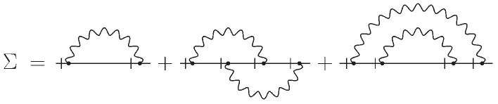
Figure 1: The self-energy operator (2.20) in the two-loop approximation.

As an example, on figure 1 we show the two-loop approximation of the self-energy operator $\Sigma$ which enters the Dyson equation

$$\langle\theta^{\prime}\theta\rangle_{\rm 1-ir}(\omega,{\bf p})=-\left\{-{\rm i}\omega+\nu_{0}p_{\bot}^{2}+\nu_{0}f_{0}p^{2}_{\parallel}\right\}+\Sigma(\omega,{\bf p})$$ (2.20)

for the 1-irreducible Green function $\langle\theta^{\prime}\theta\rangle_{\rm 1-ir}$ in the frequency–momentum representation. The wavy lines denote the velocity correlator $\langle vv\rangle_{0}$, while the solid lines correspond to the function $\langle\theta\theta^{\prime}\rangle_{0}$; the slashes mark the field $\theta^{\prime}$.

3 Canonical dimensions, UV divergences and renormalization

The analysis of UV divergences is based on the analysis of canonical dimensions of the 1-irreducible Green functions. In general, dynamic models have two scales: canonical dimension of some quantity $F$ (a field or a parameter in the action functional) is completely characterized by two numbers, the frequency dimension $d_{F}^{\omega}$ and the momentum dimension $d_{F}^{k}$; see e.g. chap. 5 in [27]. They are determined such that $[F]\sim[T]^{-d_{F}^{\omega}}[L]^{-d_{F}^{k}}$, where $L$ is some length scale and $T$ is the time scale.

Our strongly anisotropic model, however, has two independent length scales, related to the directions perpendicular and parallel to the vector ${\bf n}$, and requires a more detailed specification of the canonical dimensions. Namely, one has to introduce two independent momentum canonical dimensions $d_{F}^{\bot}$ and $d_{F}^{\parallel}$ so that

$$[F]\sim[T]^{-d_{F}^{\omega}}[L_{\bot}]^{-d_{F}^{\bot}}[L_{\parallel}]^{-d_{F}^{\parallel}},$$

where $L_{\bot}$ and $L_{\parallel}$ are (independent) length scales in the corresponding subspaces. The dimensions are found from the obvious normalization conditions $d_{k_{\bot}}^{\bot}=-d_{\bf x_{\bot}}^{\bot}=1$, $d_{k_{\bot}}^{\parallel}=-d_{\bf x_{\bot}}^{\parallel}=0$, $d_{k_{\bot}}^{\omega}=d_{k_{\parallel}}^{\omega}=0$, $d_{\omega}^{\omega}=-d_{t}^{\omega}=1$, and so on, and from the requirement that each term of the action functional (2.11) be dimensionless (with respect to all the three independent dimensions separately). The total momentum dimension can be found from the relation $d_{F}^{k}=d_{F}^{\bot}+d_{F}^{\parallel}$. Then, based on $d_{F}^{k}$ and $d_{F}^{\omega}$, one can introduce the total canonical dimension $d_{F}=d_{F}^{k}+2d_{F}^{\omega}=d_{F}^{\bot}+d_{F}^{\parallel}+2d_{F}^{\omega}$ (in the free theory, $\partial_{t}\propto\partial^{2}_{\bot}\propto\partial^{2}_{\parallel}$), which plays in the theory of renormalization of dynamic models the same role as the conventional (momentum) dimension does in static problems.

Table 1: Canonical dimensions of the fields and parameters in the model (2.11)

$F$	$\theta^{\prime}$	$\theta$	${\bf v}$	$m,\mu,\Lambda$	$\nu,\nu_{0}$	$f,f_{0}$	$w_{0}$	$w$
$d_{F}^{\omega}$	1/2	$-1/2$	1	0	1	0	0	0
$d_{F}^{\parallel}$	1	0	$-1$	0	0	$-2$	0	0
$d_{F}^{\bot}$	$d-1$	0	0	1	$-2$	2	$\xi$	0
$d_{F}^{k}=d_{F}^{\parallel}+d_{F}^{\bot}$	$d$	0	$-1$	1	$-2$	0	$\xi$	0
$d_{F}=d_{F}^{k}+2d_{F}^{\omega}$	$d+1$	$-1$	1	1	0	0	$\xi$	0

The canonical dimensions of the model (2.11) are given in table 1, including renormalized parameters, which will be introduced a bit later. From table 1 it follows that our model is logarithmic (the coupling constant $w_{0}\sim[L_{\bot}]^{-\xi}$ is dimensionless) at $\xi=0$, so that the UV divergences manifest themselves as poles in $\xi$ in the Green functions.

The total canonical dimension of an arbitrary 1-irreducible Green function $\Gamma=\langle\Phi\dots\Phi\rangle_{\rm 1-ir}$ is given by the relation

$$d_{\Gamma}=d+2-\sum_{\Phi}N_{\Phi}d_{\Phi}=d+2-N_{\theta^{\prime}}d_{\theta^{\prime}}-N_{\theta}d_{\theta}-N_{v}d_{v}.$$ (3.1)

Here $N_{\Phi}=\{N_{\theta},\,N_{\theta^{\prime}},\,N_{v}\}$ are the numbers of corresponding fields entering the function $\Gamma$, and the summation over all types of the fields in (3.1) and analogous formulas below is always implied.

Superficial UV divergences, whose removal requires counterterms, can be present only in those functions $\Gamma$ for which the ‘formal index of divergence’ $d_{\Gamma}$ is a nonnegative integer. Dimensional analysis should be augmented by the following observations:

(1) In any dynamical model of the type (2.11), 1-irreducible diagrams with $N_{\theta^{\prime}}=0$ contain closed contours of retarded propagators (2.16) and therefore vanish.

(2) For any 1-irreducible Green function $N_{\theta^{\prime}}-N_{\theta}=2N_{0}$, where $N_{0}\geq 0$ is the total number of the bare propagators $\langle\theta\theta\rangle_{0}$ entering into any of its diagrams. This fact is easily checked for any given function; it is illustrated by the function (2.20) with $N_{\theta^{\prime}}=N_{\theta}=1$ and $N_{0}=0$; see figure 1. Obviously, no diagrams with $N_{0}<0$ can be constructed. Therefore, the difference $N_{\theta^{\prime}}-N_{\theta}$ is an even nonnegative integer for any nonvanishing function.

(3) The derivative $\partial_{\parallel}$ at the vertex $\theta^{\prime}v\partial_{\parallel}\theta$ can be moved onto the field $\theta^{\prime}$ due to the transversality of $v$, see (2.13). Therefore, in any 1-irreducible diagram it is always possible to move the derivative onto any of the external ‘tails’ $\theta$ or $\theta^{\prime}$, which reduces the real index of divergence: $d_{\Gamma}^{\prime}=d_{\Gamma}-N_{\theta}-N_{\theta^{\prime}}$. The fields $\theta$, $\theta^{\prime}$ enter into the counterterms only in the form of derivatives $\partial_{\parallel}\theta$, $\partial_{\parallel}\theta^{\prime}$.

From table 1 and (3.1) we find

$$d_{\Gamma}=d+2-(d+1)N_{\theta^{\prime}}+N_{\theta}-N_{v},\quad d_{\Gamma}\!\!^{\prime}=(d+2)(1-N_{\theta^{\prime}})-N_{v}.$$ (3.2)

From these expressions we conclude that for any $d$, superficial divergences can be present only in the 1-irreducible functions $\langle\theta^{\prime}\theta\dots\theta\rangle_{\rm 1-ir}$ with $N_{\theta^{\prime}}=1$ and arbitrary $N_{\theta}$, for which $d_{\Gamma}=2$, $d_{\Gamma}^{\prime}=0$. However, all functions with $N_{\theta}>N_{\theta^{\prime}}$ vanish (see above) and obviously do not require counterterms. We are left with the only superficially divergent function $\langle\theta^{\prime}\theta\rangle_{\rm 1-ir}$; the corresponding counterterm must contain two symbols $\partial_{\parallel}$ and therefore reduces to $\theta^{\prime}\partial_{\parallel}^{2}\theta$.

Inclusion of this counterterm is reproduced by the multiplicative renormalization of the action (2.11) with the only independent renormalization constant $Z_{f}$:

$$\nu_{0}=\nu,\quad f_{0}=fZ_{f},\quad w_{0}=w\mu^{\xi}Z_{w},\quad Z_{w}=Z_{f}^{-1}.$$ (3.3)

Here the reference scale $\mu$ is an additional parameter of the renormalized theory, $\nu$, $f$ and $w$ are renormalized analogs of the bare parameters (with the subscript ‘0’) and $Z=Z(w,\xi,d)$ are the renormalization constants. Their relation in (3.3) results from the absence of renormalization of the contribution with $D_{0}$ in (2.11), so that

$$D_{0}=w_{0}\nu_{0}f_{0}=w\mu^{\xi}\nu f,$$ (3.4)

see (2.19). No renormalization of the fields and the parameter $m$ is required:

$$m_{0}=m,\quad Z_{m}=1,\quad Z_{\Phi}=1\quad{\rm for\ all}\ \Phi.$$ (3.5)

Here and below we use the minimal subtraction (MS) scheme, where all renormalization constants have the forms ‘1 + only poles in $\xi$.’

The constant $Z_{f}$ is determined by the requirement that the function $\langle\theta^{\prime}\theta\rangle_{\rm 1-ir}$, expressed in renormalized variables, be UV finite, that is, finite at $\xi=0$. We recall that the correlator $\langle vv\rangle_{0}$ contains the $\delta$ function in time, while the propagator (2.16) contains the step function. Thus all the multiloop diagrams in the self-energy operator $\Sigma$ in (2.20) contain self-contracted chains of the step functions, like e.g. $\Theta(t_{1}-t_{2})\Theta(t_{2}-t_{3})\Theta(t_{3}-t_{1})$, and therefore vanish. (In the frequency representation, all the integrands have the poles in $\omega$ only in the lower complex half-plane.) This means that the functions $\Sigma$ and $\langle\theta^{\prime}\theta\rangle_{\rm 1-ir}$ are given exactly by the one-loop approximation.

The analytic expression for the only one-loop diagram has the form

$$\Sigma({\bf p})=\int\frac{d\omega}{2\pi}\int\frac{d{\bf k}}{(2\pi)^{d}}\,D_{v}(k)\,\frac{{\rm i}p_{\parallel}{\rm i}(p-k)_{\parallel}}{-{\rm i}\omega+\epsilon({\bf p}-{\bf k})}$$ (3.6)

with $D_{v}$ from (2.7) and $\epsilon({\bf k})$ from (2.17). This expression is independent of the external frequency. The prefactor, coming from the vertices (2.18), can be replaced with $-p_{\parallel}^{2}$ due to the presence of the factor $\delta(k_{\parallel})$ in (2.7); this is the diagrammatic analog of the relation (2.13). Integration over $\omega$ involves the indeterminacy

$$\int\frac{d\omega}{2\pi}\,\frac{1}{-{\rm i}\omega+\epsilon({\bf p}-{\bf k})}=\Theta(0),$$ (3.7)

the step function at the origin; it should be carefully resolved. In our case, the function $\delta(t-t^{\prime})$ should be understood as the limit of a narrow function which is necessarily symmetric in $t\leftrightarrow t^{\prime}$, because (2.6) is a pair correlation function. Thus the quantity in (3.7) must be unambiguously defined by half the sum of the limits: $\Theta(0)=1/2$.

The integration over $k_{\parallel}$ is trivial due to the presence of the factor $\delta(k_{\parallel})$ in (2.7). The result has the form

$$\Sigma({\bf p})=-p\,{}_{\parallel}^{2}\,\frac{D_{0}}{2}\,\int_{k_{\bot}>m}\frac{d{\bf k}_{\bot}}{(2\pi)^{(d-1)}}\,\frac{1}{k_{\bot}^{d-1+\xi}}.$$ (3.8)

The remaining integration over ${\bf k}_{\bot}$ gives

$$\Sigma({\bf p})=-p\,{}_{\parallel}^{2}\,D_{0}m^{-\xi}\,\frac{S_{d-1}}{2(2\pi)^{(d-1)}}\frac{1}{\xi},$$ (3.9)

where $S_{d}=2\pi^{d/2}/\Gamma(d/2)$ with Euler’s Gamma function is the surface area of the unit sphere in the $d$-dimensional space. Substituting the expression (3.9) into the Dyson equation (2.20) and passing to renormalized parameters with the aid of relations (3.3) and (3.4) gives

$$\langle\theta^{\prime}\theta\rangle_{\rm 1-ir}(\omega,{\bf p})=-\left\{-{\rm i}\omega+\nu p_{\bot}^{2}+\nu fZ_{f}p^{2}_{\parallel}\right\}-p\,{}_{\parallel}^{2}\frac{wf\nu S_{d-1}}{2(2\pi)^{(d-1)}}\left(\frac{\mu}{m}\right)^{\xi}\frac{1}{\xi}.$$ (3.10)

In order to cancel the pole in $\xi$, the renormalization constant in the MS scheme has to be chosen in the form

$$Z_{f}=1-\frac{w}{\xi},$$ (3.11)

where we have absorbed the factor $S_{d-1}/2(2\pi)^{(d-1)}$ into the coupling constant.

4 RG equations and the fixed point

Let $G(e_{0},\dots)$ be some correlation function in the original model (2.11) and $G_{R}(e,\mu,\dots)$ its analog in the renormalized theory. Here $e_{0}$ is the complete set of bare parameters, $e$ is the set of their renormalized counterparts, and the ellipsis stands for the other variables like the coordinates/momenta and times/frequences. These functions differ only by normalization and the choice of variables, $G(e_{0})=Z_{G}G_{R}(e,\mu)$, and can equally be used for the analysis of critical behaviour. (For the correlation functions of the primary fields $Z_{G}=1$ due to the absence of their renormalization, but it is instructive to discuss a more general case.) We use $\widetilde{\cal D}_{\mu}$ to denote the differential operation $\mu\partial_{\mu}$ for fixed $e_{0}$ and operate on both sides of the last equality with it. This gives the basic RG equation:

$$\left\{{\cal D}_{RG}+\gamma_{G}\right\}\,G^{R}(e,\mu,\dots)=0,$$ (4.1)

where ${\cal D}_{RG}$ is the operation $\widetilde{\cal D}_{\mu}$ expressed in the renormalized variables:

$${\cal D}_{RG}={\cal D}_{\mu}+\beta\partial_{w}-\gamma_{f}{\cal D}_{f}.$$ (4.2)

Here we have written ${\cal D}_{x}\equiv x\partial_{x}$ for any variable $x$, and the RG functions (the $\beta$ function and the anomalous dimensions $\gamma$) are defined as

$$\beta(w)=\widetilde{\cal D}_{\mu}w=w\,[-\xi-\gamma_{w}],$$ (4.3)

$$\gamma_{e}(u)=\widetilde{\cal D}_{\mu}\ln Z_{e}=\beta\partial_{u}\ln Z_{e}\quad{\rm for\ any\ quantity}\ e.$$ (4.4)

From the relations (3.3)–(3.5) it follows

$$\gamma_{\nu}=\gamma_{m}=\gamma_{\Phi}=0\quad{\rm and}\quad\gamma_{f}=-\gamma_{w},$$ (4.5)

while from (4.3) and (4.4) for $e=w$ one easily derives

$$\gamma_{w}(u)=\frac{-\xi{\cal D}_{w}\ln Z_{w}}{1+{\cal D}_{w}\ln Z_{w}},\quad\beta(w)=\frac{-\xi w}{1+{\cal D}_{w}\ln Z_{w}}.$$ (4.6)

Substituting (3.11) into (4.6) one obtains exact expressions

$$\gamma_{f}=-\gamma_{w}=w,\quad\beta=w[-\xi+w].$$ (4.7)

It is well known that IR asymptotic behaviour of the Green functions is governed by IR attractive fixed points of the RG equations, defined by the relations $\beta(w_{*})=0$ and $\beta^{\prime}(w_{*})>0$. From (4.7) it follows that our model has a fixed point

$$w_{*}=\xi,\quad\beta^{\prime}(w_{*})=\xi$$ (4.8)

which is positive and IR attractive for $\xi>0$. At this point

$$\gamma_{f}^{*}=-\gamma_{w}^{*}=\xi.$$ (4.9)

Here and below we denote $\gamma_{e}^{*}=\gamma_{e}(w_{*})$. We also stress that all the expressions in (4.8) and (4.9) are exact.

5 Critical scaling and critical dimensions

In the leading order of the IR asymptotic behaviour the Green functions satisfy the RG equation with the substitution $w\to w_{*}$, which gives

$$\left\{{\cal D}_{\mu}-\gamma_{f}^{*}{\cal D}_{f}+\gamma_{G}^{*}\right\}\,G^{R}(e,\mu,\dots)=0.$$ (5.1)

Canonical scale invariance of the function $G^{R}$ with respect to the three independent canonical dimensions (see section 3) can be expressed by the differential equations of the form

$$\left\{\sum_{F}d^{*}_{F}\,{\cal D}_{F}-d^{*}_{G}\right\}\,G^{R}(e,\mu,\dots)=0,$$ (5.2)

where the sum runs over all arguments of the Green function, including the coordinates/momenta and times/frequences, and $d^{*}_{F}=d_{F}^{\omega}$, $d_{F}^{\bot}$ and $d_{F}^{\parallel}$ are the corresponding canonical dimensions. In the time–coordinate representation

$$d^{*}_{G}=\sum_{\Phi}N_{\Phi}d^{*}_{\Phi}=N_{\theta^{\prime}}d^{*}_{\theta^{\prime}}+N_{\theta}d^{*}_{\theta}+N_{v}d^{*}_{v},$$ (5.3)

where $N_{\Phi}$ are the numbers of the fields entering the Green function, cf. equation (3.1). From table 1 we find

$$\left\{-{\cal D}_{t}+{\cal D}_{\nu}-d^{\omega}_{G}\right\}\,G^{R}(e,\mu,\dots) = 0,$$

$$\left\{-{\cal D}_{\bot}+{\cal D}_{\mu}-2{\cal D}_{\nu}+2{\cal D}_{f}+{\cal D}_{m}-d^{\bot}_{G}\right\}\,G^{R}(e,\mu,\dots) = 0,$$

$$\left\{-{\cal D}_{\parallel}-2{\cal D}_{f}-d^{\parallel}_{G}\right\}\,G^{R}(e,\mu,\dots) = 0,$$ (5.4)

where for definiteness we use the time–coordinate representation and denote ${\cal D}_{\bot}=x_{\bot}\partial/\partial x_{\bot}$, ${\cal D}_{\parallel}=x_{\parallel}\partial/\partial x_{\parallel}$.

The equations of the type (5.1), (5.2) and (5.4) describe the scaling behaviour of the function $G^{R}$ upon the dilation of a part of its parameters: a parameter is dilated if the corresponding derivative enters the equation; otherwise it is kept fixed. We are interested in the IR scaling behaviour, in which all the IR relevant parameters (coordinates, times, integral scale) are dilated, while the irrelevant parameters (diffusivity coefficients, coupling constant) are fixed. Thus we combine the equations (5.1) and (5.4) so that the derivatives with respect to the IR irrelevant parameters be eliminated; this gives the desired equation which describes the IR scaling behaviour:

$$\left\{{\cal D}_{\bot}+\Delta_{\parallel}{\cal D}_{\parallel}+\Delta_{\omega}{\cal D}_{\omega}+\Delta_{m}{\cal D}_{m}-\Delta_{G}\right\}G^{R}=0.$$ (5.5)

Here $\Delta_{\bot}=1$ is the normalization condition, while the critical dimensions of any other IR relevant parameter $F$ is given by the general expression

$$\Delta_{F}=d_{F}^{\bot}+\Delta_{\parallel}d_{F}^{\parallel}+\Delta_{\omega}d_{F}^{\omega}+\gamma^{*}_{F},$$ (5.6)

where

$$\Delta_{\omega}=2-\gamma_{\nu}^{*},\quad\Delta_{\parallel}=\left(2+\gamma_{f}^{*}\right)/2.$$ (5.7)

Then using (4.5), (4.9) and the data from table 1 we obtain the following exact expressions for the dimensions:

$$\Delta_{\omega}=2,\ \Delta_{\parallel}=1+\xi/2,\ \Delta_{\theta^{\prime}}=d+1+\xi/2,\ \Delta_{\theta}=-1,\ \Delta_{m}=1.$$ (5.8)

Solution of the RG equations for the structure functions (1.2) will be discussed in section 7.

6 Critical dimensions of the composite operators

The key role in the following will be played by the critical dimensions of certain composite fields (“composite operators” in quantum-field terminology). Detailed exposition of the renormalization procedure of composite operators can be found in [27]. In general, counterterms to a given operator $F$ are determined by all possible 1-irreducible Green functions with one operator $F$ and arbitrary number of primary fields, $\Gamma=\langle F(x)\Phi(x_{1})\dots\Phi(x_{2})\rangle_{\rm 1-ir}$. The total canonical dimension of this function (formal index of divergence) is

$$d_{\Gamma}=d_{F}-\sum_{\Phi}N_{\Phi}d_{\Phi},$$ (6.1)

where $d_{F}$ is the dimension of the operator and the summation over all types of fields is implied, cf. expression (3.1). For superficially divergent diagrams $d_{\Gamma}$ is a nonnegative integer.

We begin with the simplest operators $\theta^{n}(x)$, which enter the structure functions (1.2). Using the data in table 1 we obtain $d_{F}=nd_{\theta}=-n$ and $d_{\Gamma}=-n+N_{\theta}-N_{v}-(d+1)N_{\theta^{\prime}}$. From the analysis of the diagrams it follows that the total number of the fields $\theta$ entering the function $\Gamma$ cannot exceed the number of the fields $\theta$ in the operator $\theta^{n}$ itself, that is, $N_{\theta}\leq n$. This is a direct consequence of the linearity of the original stochastic equation (2.1) in the field $\theta$: the solid lines in the diagrams cannot branch. Therefore, the superficial divergence can only exist in the functions with $N_{v}=N_{\theta^{\prime}}=0$ and arbitrary value of $n=N_{\theta}$, for which the formal index vanishes, $d_{\Gamma}=0$. However, in any nontrivial diagram at least one of $N_{\theta}$ external ‘tails’ of the field $\theta$ is attached to a vertex $\theta^{\prime}(v\partial)\theta$, at least one derivative $\partial$ appears as an extra factor in the diagram, and, consequently, the real index of divergence $d_{\Gamma}^{\prime}$ is necessarily negative.

This means that the operator $\theta^{n}$ is in fact UV finite and requires no counterterms at all: $\theta^{n}=Z\,[\theta^{n}]_{R}$ with $Z=1$. It then follows that its critical dimension, given by the expression (5.6) without the contribution of $\gamma_{F}^{*}$, is simply given by the sum of the critical dimensions of its constituents:

$$\Delta[\theta^{n}]=n\Delta_{\theta}=-n.$$ (6.2)

In Kraichnan’s rapid-change model, the anomalous exponents (1.4) are identified with the critical dimensions of the scalar composite operators of the form $(\partial\theta)^{2n}$, the operators with minimal canonical dimension (namely, $d_{F}=0$) that are invariant with respect to the shift $\theta\to\theta+{\rm const}$; see [6]–[7]. For that isotropic case, the scalar operator of the needed form is unique for any given $n$: $F_{n}=(\partial_{i}\theta\partial_{i}\theta)^{n}$. The operator $F_{n}$ does not admix in renormalization to $F_{k}$ with $k<n$, the corresponding renormalization matrix is triangular, and the dimensions $\Delta_{n}$ are determined by its diagonal elements. (The operators $F_{n}$ can be treated as if they were multiplicatively renormalizable.) For the existence of the singular behaviour of the structure functions (1.3) at $(r/{\cal L})\to 0$ it is crucial that the dimensions $\Delta_{n}$ are negative.

In our case the $O_{d}$ isotropy is broken to $O_{d-1}\otimes Z_{2}$, and for any $n$ one can construct a set of $(n+1)$ different operators of the form $(\partial\theta)^{2n}$, invariant under the residual symmetry, namely:

$$F_{k,s}=(\partial_{i}^{\bot}\theta\partial_{i}^{\bot}\theta)^{k}(\partial_{\parallel}\theta\partial_{\parallel}\theta)^{s},\quad k+s=n.$$ (6.3)

Here $\partial_{i}^{\bot}$ is the derivative in the ${\bf x}_{\bot}$ subspace, $\partial_{\parallel}=\partial/\partial x_{\parallel}$ and the summation over the vector index $i=1,\dots,d-1$ is implied. In particular, for $n=1$ such a set includes two operators

$$F_{1,0}=(\partial_{i}^{\bot}\theta\partial_{i}^{\bot}\theta),\quad F_{0,1}=(\partial_{\parallel}\theta)^{2},$$ (6.4)

for $n=2$ — three operators

$$F_{2,0}=(\partial_{i}^{\bot}\theta\partial_{i}^{\bot}\theta)^{2},\quad F_{1,1}=(\partial_{i}^{\bot}\theta\partial_{i}^{\bot}\theta)(\partial_{\parallel}\theta)^{2},\quad F_{0,2}=(\partial_{\parallel}\theta)^{4},$$ (6.5)

and so on.

For all operators (6.3), from table 1 and equation (6.1) we find $d_{F}=0$ and $d_{\Gamma}=N_{\theta}-N_{v}-(d+1)N_{\theta^{\prime}}$, with the necessary condition $N_{\theta}\leq 2n=2(k+s)$, following from the linearity of the model (cf. the discussion for $\theta^{n}$ above). From the form of the vertex $\theta^{\prime}(v\partial)\theta$ and the operators $F_{k,s}$ themselves it follows that the fields $\theta$, $\theta^{\prime}$ enter the counterterms only in the form of derivatives, $\partial\theta$, $\partial\theta^{\prime}$, so that the real index of divergence is $d_{\Gamma}^{\prime}=d_{\Gamma}-N_{\theta}-N_{\theta^{\prime}}=-N_{v}-(d+2)N_{\theta^{\prime}}$. Thus the superficial divergences can only exist in the Green functions with $N_{v}=N_{\theta^{\prime}}=0$ and arbitrary $N_{\theta}\leq 2n$ (then $d_{\Gamma}^{\prime}=0$), and the corresponding operator counterterm necessarily reduces to the form $F_{m,l}$ with $(m+l)\leq(k+s)$.

Therefore, the operators of the type $F_{k,s}$ can mix only with each other in renormalization, the corresponding infinite renormalization matrix $Z=\{Z_{k,s;m,l}\}$ is in fact block-triangular, $Z_{k,s;m,l}=0$ for $(m+l)>(k+s)$, and the critical dimensions associated with the set of operators with given $n=(k+s)$ are determined by its finite diagonal blocks $Z_{n}=\{Z_{k,s;m,l}\}$ with the fixed value of the sum $n=(m+l)=(k+s)$.

In the following, we will show that the counterterms and the renormalization matrices for these operators are fully specified by the one-loop approximations.

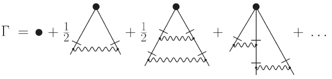
Figure 2: The one-loop and a part of the two-loop contributions to the generating functional (LABEL:GrandFunk).

It is convenient to work with the generating functional of 1-irreducible correlation functions with one operator $F_{k,s}$ and arbitrary number of the primary fields $\theta$:

$$\Gamma_{k,s}(x;\theta)=\sum_{p=0}^{\infty}\int dx_{1}\dots\int dx_{p}\bigg{\langle}F_{k,s}(x)\theta(x_{1})\cdots\theta(x_{p})\bigg{\rangle}_{\rm 1-ir}\theta(x_{1})\cdots\theta(x_{p}).$$

In the diagrammatic expansion of the functional $\Gamma_{k,s}$, the leading (loopless) approximation is given by the operator $F_{k,s}(x)$ itself. The only one-loop diagram and two of the five two-loop diagrams are shown in figure 2. The diagrammatic notation was explained in section 3 in connection with figure 1; the new elements are the thick dots that denote the vertex factors of the composite field $F_{k,s}$:

$$V^{(l)}_{k,s}(x;x_{1},\dots,x_{l})=\frac{\delta^{l}F_{k,s}(x)}{\delta\theta(x_{1})\cdots\delta\theta(x_{l})},$$ (6.7)

where $l$ is the number of $\langle\theta\theta^{\prime}\rangle_{0}$-lines attached to the vertex (6.7). The variational derivative acts on such operators as follows:

$$\frac{\delta}{\delta\theta(x^{\prime})}F_{k,s}(x) = 2k\,F_{k-1,s}(x)\,\partial_{i}^{\bot}\theta(x)\,\partial_{i}^{\bot}\delta(x-x^{\prime})+$$ (6.8)

$$+ 2s\,F_{k,s-1}(x)\,\partial_{\parallel}\theta(x)\partial_{\parallel}\delta(x-x^{\prime}),$$

so that the vertex factor (6.7) is in fact local.

The derivatives $\partial_{\parallel}$ at the external vertices (two lower vertices in the first two diagrams on figure 2 and three lower vertices in the last diagram) correspond to external momenta; they act onto the fields $\theta$ attached to those vertices and form the external factors $\sim(\partial_{\parallel}\theta)^{l}$. The remaining expressions diverge logarithmically and therefore can be calculated at all external momenta equal to zero; the IR regularization is provided by the cutoff $m$ in the velocity correlator (2.7).

It is easy to see that the number of independent loops in any diagram of the functional (LABEL:GrandFunk) equals to the number of wavy lines; thus the independent integration momenta (denoted as ${\bf k}$ and ${\bf q}$ below) can always be assigned to the velocity correlators. Then the integrals corresponding to the diagrams in figure 2 take on the forms:

$$\int\frac{d{\bf k}}{(2\pi)^{d}}\int\frac{d\omega}{2\pi}\frac{k_{i}k_{j}}{(\omega^{2}+\epsilon^{2}({\bf k}))}\left[D_{v}(k)(\partial_{\parallel}\theta(x))^{2}\right]$$ (6.9)

for the one-loop diagram,

$$\int\frac{d{\bf k}}{(2\pi)^{d}}\int\frac{d{\bf q}}{(2\pi)^{d}}\int\frac{d\omega}{2\pi}\int\frac{d\Omega}{2\pi}\,\left[D_{v}(k)q^{2}_{\parallel}\right]\left[D_{v}(q)(\partial_{\parallel}\theta(x))^{2}\right]\times$$

$$\times\frac{(k+q)_{i}(k+q)_{j}}{\left\{\omega^{2}+\epsilon^{2}({\bf k}+{\bf q})+\epsilon^{2}({\bf q})\right\}\left\{\Omega^{2}+\epsilon^{2}({\bf q})\right\}}$$ (6.10)

for the first two-loop diagram and

$$\int\frac{d{\bf k}}{(2\pi)^{d}}\int\frac{d{\bf q}}{(2\pi)^{d}}\int\frac{d\omega}{2\pi}\int\frac{d\Omega}{2\pi}\,\left[D_{v}(k)({\rm i}q_{\parallel}\partial_{\parallel}\theta(x))\right]\left[D_{v}(q)(\partial_{\parallel}\theta(x))^{2}\right]\times$$

$$\times\frac{{\rm i}k_{i}q_{j}(k+q)_{l}}{\left\{\Omega^{2}+\epsilon^{2}({\bf q})\right\}\left\{-{\rm i}\omega+\epsilon({\bf k})\right\}\left\{{\rm i}(\omega+\Omega)+\epsilon({\bf k}+{\bf q})\right\}}$$ (6.11)

for the last one. Here $\epsilon({\bf k})=\nu(k_{\bot}^{2}+fk_{\parallel}^{2})$ is the renormalized analog of the quantity from (2.17).

The momenta with free vector indices stem from the vertex factor (6.7) and correspond to the derivatives acting onto the spatial $\delta$ functions in expressions like (6.8). Each factor in square brackets comes from one velocity correlator (2.6) and two vertices (2.18) attached to it; $D_{v}$ being the function (2.7). Thus the integrand for any diagram contains the factor $D_{v}(k)\sim\delta(k_{\parallel})$ for each independent integration momentum ${\bf k}$. On the other hand, any diagram of the functional (LABEL:GrandFunk) with more than one loop necessarily contains at least one internal vertex (2.18), the corresponding vertex factor is proportional to certain linear combination of independent parallel momenta $k_{\parallel}$, $q_{\parallel}$ and so on, and the integrand as a whole vanishes due to the presence of the corresponding $\delta$ functions (we recall that all the external momenta are set equal to zero). Thus the only contribution to the counterterm comes from the one-loop diagram. For the same reason, the integral (6.9) is nontrivial only if the both momenta in the factor $k_{i}k_{j}$ are perpendicular to the vector ${\bf n}$; otherwise $k_{i}=n_{i}k_{\parallel}$ and the above mechanism works. So one can replace $k_{i}\to k_{i}^{\bot}$ in (6.9), and in the vertex keep only the term

$$V^{(2)}_{k,s}(x;x_{1},x_{2})\simeq F_{0,s}(x)\frac{\delta^{2}}{\delta\theta(x_{1})\delta\theta(x_{2})}F_{k,0}(x).$$ (6.12)

Thus the operator $F_{k,s}$ in the divergent part of the one-loop diagram loses two factors $\partial^{\bot}\theta$ in (6.12) and acquires two factors $\partial_{\parallel}\theta$ in (6.9), so that the counterterm to the functional (LABEL:GrandFunk) reduces to the form $F_{k-1,s+1}$. We conclude that the renormalized operator corresponding to $F_{k,s}$ has the form $F^{R}_{k,s}=F_{k,s}+aF_{k-1,s+1}$. Resolving these relations for $F_{k,s}$ gives

$$F_{k,s}=F^{R}_{k,s}+\sum_{l=1}^{l=k}a_{l}F^{R}_{k-l,s+l}$$ (6.13)

with some coefficients $a_{l}$ and $a_{1}=-a$. Thus the renormalization matrix $Z_{n}=\{Z_{k,s;m,l}\}$ in the matrix relation $F=Z_{n}F^{R}$ is triangular (with a natural numbering of operators in the family with fixed $k+s=n$) and its diagonal elements are all equal to unity, $Z_{k,s;k,s}=1$. The other nonvanishing elements $Z_{k,s;k-l,s+l}$ are determined by the one-loop diagram (6.9), but we will not need their explicit expressions. Indeed, the matrix of critical dimensions for the operators (6.3) is given by the expressions (5.6)–(5.8), in which $d_{F}^{*}$ should be understood as diagonal matrices of canonical dimensions of the operators $F_{k,s}$ and $\gamma_{F}=Z_{n}^{-1}\widetilde{\cal D}_{\mu}Z_{n}$ is the matrix of their anomalous dimensions. The latter is triangular with vanishing diagonal elements $\gamma_{k,s;k,s}=0$ and nontrivial $\gamma_{k,s;k-l,s+l}$ with $k=1,\dots,l$. Thus the critical dimensions $\Delta_{k,s}$ related to the set $F_{k,s}$, given by the eigenvalues of the matrix (5.6), coincide with its diagonal elements. From table 1 for the operators $F_{k,s}$ we find

$$d_{F}^{\bot}=2k,\quad d_{F}^{\parallel}=2s,\quad d_{F}^{\omega}=-(k+s),$$

so that

$$\Delta_{k,s}=2k+2s\Delta_{\parallel}-(k+s)\Delta_{\omega}$$

with no contribution from $\gamma^{*}_{F}$, which along with expressions (5.8) gives the final exact result

$$\Delta_{k,s}=s\xi$$ (6.14)

for the critical dimensions related to the operators (6.3). In contrast to the result (1.4) for the isotropic Kraichnan’s model, they have no corrections of order $O(\xi^{2})$ and higher and are positive for all $k$, $s$ and $\xi>0$.

7 RG and the IR scaling behaviour of the structure functions

The results of the preceding sections allow one to find the IR scaling behaviour of the correlation functions in our model. For generality, consider the different-time structure functions

$$S_{2n}(\tau,r_{\bot},r_{\parallel})=\langle\left[\theta(t,{\bf x})-\theta(t^{\prime},{\bf x}^{\prime})\right]^{2n}\rangle,$$ (7.1)

where $\tau=t^{\prime}-t$, $r_{\bot}=|{\bf x}_{\bot}-{\bf x}^{\prime}_{\bot}|$ and $r_{\parallel}=|x_{\parallel}-x_{\parallel}^{\prime}|$. The equal-time functions (1.2) are obtained for $\tau=0$.

The function (7.1) is a linear combination of the two-point correlators $\langle\theta^{k}(t,{\bf x})\theta^{s}(t^{\prime},{\bf x}^{\prime})\rangle$ with the fixed $k+s=2n$. Due to simple exact relations (6.2) for the dimensions of the operators $\theta^{n}$, the critical dimensions of these correlators are all equal, $\Delta_{k}+\Delta_{s}=-(k+s)=-2n=2n\Delta_{\theta}$, and the function $S_{2n}$ in the IR range behaves as a single object. Its IR scaling form can be easily written using the IR scaling equation (5.5) with known critical dimensions (5.8) of the basic IR relevant parameters, but it is instructive to discuss its derivation from the RG equation in more detail.

From the dimensional considerations one can write

$$S_{2n}=\nu^{-n}r_{\bot}^{2n}{\cal F}\left(\mu r_{\bot},w,r_{\parallel}/f^{1/2}r_{\bot},\nu\tau r_{\bot}^{2},mr_{\bot}\right),$$ (7.2)

where ${\cal F}(\dots)$ are some functions of completely dimensionless arguments (that is, dimensionless with respect to all the canonical dimensions $d_{F}^{*}$ separately; see section 3).

Since the operators $\theta^{n}$ are not renormalized, the function $S_{2n}$ satisfies the homogeneous RG equation (4.1) with $\gamma_{G}=0$. Its solution can be represented in the form

$$S_{2n}=\bar{\nu}^{-n}r_{\bot}^{2n}{\cal F}\left(1,\bar{w},r_{\parallel}/\bar{f}^{1/2}r_{\bot},\bar{\nu}\tau/r_{\bot}^{2},\bar{m}r_{\bot}\right),$$ (7.3)

with the same functions ${\cal F}$. The invariant variables $\bar{e}$ are solutions of the homogeneous equation (4.1) normalized with respect to $e$ at $\mu r_{\bot}=1$. They can be expressed in the original (bare) parameters $e_{0}$ using the relations

$$w_{0}=\bar{w}r_{\bot}^{-\xi}Z_{w}(\bar{w}),\quad f_{0}=\bar{f}Z_{f}(\bar{w}),\quad\bar{\nu}=\nu_{0},\quad\bar{m}=m_{0},$$ (7.4)

with the renormalization constants from (3.3) and (3.5). The representations (7.3) and (7.4) are valid because both their sides satisfy the same RG equation and coincide in the normalization point $\mu r_{\bot}=1$ due to the definition of $\bar{e}$ and the relations (3.3). The simple result for $\bar{\nu}$ and $\bar{m}$ follows from the fact that these parameters are not renormalized.

The advantage of the representation (7.3) is that the invariant variables have simple asymptotic behaviour for $\Lambda r_{\bot}\to\infty$ (or $\mu r_{\bot}\to\infty$ in renormalized variables). The exact explicit expression for the invariant charge

$$\bar{w}=w_{*}\left[1+w_{*}r_{\bot}^{-\xi}/w_{0}\right]^{-1}$$ (7.5)

is derived from the relations (3.3), (3.11) and (7.4). From (7.5) it follows that, for $\xi>0$ and $r_{\bot}\to\infty$, the invariant charge tends to the IR attractive fixed point of the RG equation: $\bar{w}\to w_{*}=\xi$. For $\bar{f}$, eliminating the renormalization constant $Z_{w}=Z_{f}^{-1}$ from (7.4) gives

$$\bar{f}=f_{0}w_{0}r_{\bot}^{\xi}/\bar{w}\to f_{0}w_{0}r_{\bot}^{\xi}/w_{*}.$$ (7.6)

Substituting these expressions into (7.3) gives the desired asymptotic expression for the structure functions in the IR range $\Lambda r_{\bot}\gg 1$:

$$S_{2n}=\nu_{0}^{-n}r_{\bot}^{2n}{\cal F}\left(1,w_{*},r_{\parallel}/(f_{0}w_{0})^{1/2}r_{\bot}^{1+\xi/2},\nu_{0}\tau/r_{\bot}^{2},mr_{\bot}\right).$$ (7.7)

It can be made more transparent by discarding in the notation all the IR irrelevant parameters:

$$S_{2n} = r_{\bot}^{2n}{\cal R}\left(r_{\parallel}r_{\bot}^{-1-\xi/2},\tau/r_{\bot}^{2},mr_{\bot}\right)=$$ (7.8)

$$= r_{\bot}^{-2n\Delta_{\theta}}{\cal R}\left(r_{\parallel}/r_{\bot}^{\Delta_{\parallel}},\tau/r_{\bot}^{\Delta_{\omega}},mr_{\bot}^{\Delta_{m}}\right)$$

with certain scaling functions ${\cal R}$. Of course, the last expression, in which we have used the explicit forms (5.8) of the critical dimensions, could be derived directly from the general IR scaling equation (5.5), but the more detailed representation (7.7) gives additional interesting information about the dependence on the IR irrelevant papameters.

In the isotropic Kraichnan’s model, the structure functions in the IR range $\Lambda r_{\bot}\gg 1$ depend only on the IR (integral) scale ${\cal L}=1/m$ and the amplitude $D_{0}=w_{0}\nu_{0}$ entering the velocity correlator (1.1), but not on the diffusivity coefficient $\nu_{0}$ and the coupling constant $w_{0}\sim\Lambda^{\xi}$ separately; see (1.3). The same effect takes place for the stochastic Navier–Stokes equation; see e.g. the discussion in chapter 6 of [27]. This fact is in agreement with the second Kolmogorov hypothesis about the independence of the correlation functions in the IR range of the parameters, related to the UV (dissipation) scale: viscosity coefficient for the velocity and diffusivity coefficient for the passive scalar field; see e.g. [2]. In the case at hand, the UV parameters $\nu_{0}$, $f_{0}$ and $w_{0}\sim\ell^{-\xi}$ survive in the IR asymptotic expression (7.7) for the structure functions (they do not form the combination $D_{0}=w_{0}\nu_{0}f_{0}$ even if we set $f_{0}=1$). Thus we may conclude that, in contrast to the isotropic case, the second Kolmogorov hypothesis is invalid for the shear flow.

8 OPE and the inertial-range behaviour of the structure functions

The asymptotic representations (7.7) and (7.8) hold in the IR asymtotic range, specified by the inequality $\Lambda r_{\bot}\gg 1$ (or $\mu r_{\bot}\gg 1$ in renormalized variables), while the other arguments of the scaling functions ${\cal R}$ are kept finite. Inertial range corresponds to the additional condition $mr_{\bot}\ll 1$. The form of the scaling functions ${\cal F}$ or ${\cal R}$ is not determined by the RG equations alone. In order to study the limit $mr_{\bot}\to 0$ in the structure functions, one should combine the plain RG with the OPE techniques; see [6]–[7] for Kraichnan’s model. For simplicity, below we concentrate on the equal-time functions, setting $\tau=0$ in (7.7) and (7.8).

According to the OPE, the behaviour of the quantities entering into the structure functions (1.2) for ${\bf r}={\bf x}-{\bf x^{\prime}}\to 0$ and fixed ${\bf x}+{\bf x^{\prime}}$ is given by the infinite sum

$$\left[\theta(t,{\bf x})-\theta(t,{\bf x^{\prime}})\right]^{n}=\sum_{F}C_{F}({\bf r})F\left(t,\,\frac{{\bf x}+{\bf x^{\prime}}}{2}\right),$$ (8.1)

where $C_{F}$ are coefficients regular in $m^{2}$ and $F$ are all possible renormalized local composite operators allowed by the symmetry. More precisely, the operators entering the OPE are those which appear in the plain Taylor expansion, and all the operators that admix to them in renormalization.

The structure functions (1.2) are obtained by averaging equation (8.1) with the weight $\exp{\cal S}_{R}$, where ${\cal S}_{R}$ is the renormalized action; the mean values $\langle F\rangle$ appear on the right-hand side. Their asymptotic behaviour for $m\to 0$ is found from the corresponding RG equations and has the form $\langle F\rangle\propto m^{\Delta_{F}}$. Then substituting the OPE into the asymptotic expression (7.8) gives

$$S_{2n}({\bf r})=r_{\bot}^{2n}\sum_{F}A_{F}\left(r_{\parallel}/r_{\bot}^{\Delta_{\parallel}},mr_{\bot}\right)\,(mr_{\bot})^{\Delta_{F}},$$ (8.2)

with coefficients $A_{F}$ regular in $(mr_{\bot})^{2}$.

Due to the linearity of the model, the number of the fields $\theta$ in such operators $F$ cannot exceed their number in the left-hand side. Due to the invariance of the action functional (2.11) and the quantity in (8.1) with respect to the shift of the field, $\theta\to\theta+{\rm const}$, the operators entering the OPE must also obey this symmetry. It can always be assumed that the expansion (8.1) is made in irreducible tensors (scalars, vectors and traceless tensors); owing to the symmetries of our model, only contributions of the scalar operators survive in (8.2). The leading contributions are determined by the operators with minimal critical dimensions $\Delta_{F}=d_{F}+O(\xi)$.

It then follows that the leading terms of the small-$mr_{\bot}$ behaviour of the expression (8.2) for the function $S_{2n}$ are given by the scalar operators $F_{k,s}$ from (6.3) with $k+s\leq n$. Their dimensions $\Delta_{k,s}=s\xi$ in (6.14) are all nonnegative; the leading term is given by the operators with $s=0$ (including the simplest $F=1$), the operators with $s\geq 1$ determine the corrections vanishing for $mr_{\bot}\to 0$.

We conclude that the function $S_{2n}$ remains finite at $m=0$. Thus in the inertial range and for $\tau=0$ expression (7.8) becomes

$$S_{2n}=r_{\bot}^{-2n\Delta_{\theta}}{\cal R}\left(r_{\parallel}/r_{\bot}^{\Delta_{\parallel}}\right),$$ (8.3)

which for $r_{\parallel}=0$ turns to the simple power law

$$S_{2n}\sim r_{\bot}^{-2n\Delta_{\theta}}=r_{\bot}^{2n},$$ (8.4)

while for $r_{\bot}=0$ one obtains

$$S_{2n}\sim r_{\parallel}^{-2n\Delta_{\theta}/\Delta_{\parallel}}=r_{\parallel}^{2n/(1+\xi/2)}.$$ (8.5)

Thus the inertial-range behaviour in the rapid-change model of a shear flow differs essentially from that in the isotropic model. In contrast to the behaviour (1.3), (1.4) of the latter, singular at $mr\to 0$, there is no anomalous (multi)scaling in the case at hand.

9 Finite correlation time

In this section we will consider the case of the Gaussian velocity field with a finite correlation time. Now the function $\widetilde{D}_{v}$ in the correlator (2.6), (2.7) depends on frequency $\omega$ and will be chosen in the form

$$\widetilde{D}_{v}(\omega,k_{\bot})=\frac{g_{0}\nu_{0}^{3}f_{0}\,k_{\bot}^{5-d-(\varepsilon+\eta)}}{\omega^{2}+[u_{0}\nu_{0}k_{\bot}^{2-\eta}]^{2}}.$$ (9.1)

The function (9.1) involves two independent exponents $\eta$ and $\varepsilon$, which in the RG approach play the role of two formal expansion parameters. The former defines the dispersion law $\omega(k_{\bot})\sim k_{\bot}^{2-\eta}$ ($z=2-\eta$ in the notation of [9]–[19]), while the latter governs the behaviour of the one-dimensional velocity spectrum, related to the equal-time correlator:

$${\cal E}(k_{\bot})\sim k_{\bot}^{d-2}\int\frac{d\omega}{2\pi}\widetilde{D}_{v}(\omega,k_{\bot})=(g_{0}f_{0}\nu_{0}^{2}/2u_{0})k_{\bot}^{1-\varepsilon};$$ (9.2)

this explains the choice of the exponent in the numerator of (9.1).

The correlator (9.1) involves two important special cases, which, as we will see, nearly exhaust possible IR behaviour of the model. The limit $u_{0}\to 0$ at fixed $g_{0}^{\prime}=g_{0}/u_{0}$ corresponds to the case of time-independent (‘frozen’) velocity field, when (9.1) turns to $\widetilde{D}_{v}\sim\delta(\omega)k^{3-d-\varepsilon}$. The limit $u_{0}\to\infty$ at fixed $g_{0}^{\prime\prime}=g_{0}/u^{2}_{0}$ returns us to the rapid-change case (2.6), (2.7) with $\xi=\varepsilon-\eta$ and $w_{0}=g_{0}^{\prime\prime}$.

The role of coupling constants will be played by the parameters (see below)

$$g_{0}\sim\Lambda^{\varepsilon+\eta}\sim\Lambda^{\xi+2\eta},\quad u_{0}\sim\Lambda^{\eta},\quad g_{0}^{\prime}\sim\Lambda^{\varepsilon},\quad g_{0}^{\prime\prime}\sim\Lambda^{\xi},$$ (9.3)

where $\Lambda$ is a typical UV momentum scale, cf. (2.19). The model is logarithmic (the couplings in (9.3) are all dimensionless) at $\eta=\varepsilon=0$, so that the UV divergences manifest themselves as poles in $\eta$, $\varepsilon$ and their linear combinations.

As a rule, synthetic velocity ensembles with a finite correlation time suffer from the lack of Galilean invariance, which can lead to some physical pathologies; see e.g. the discussion in [28]. Surprisingly enough, in our strongly anisotropic case the action functional (2.11) with the correlator (9.1) in (2.14) is invariant with respect to the Galilean transformation of the fields

$$\theta(t,{\bf x})\to\theta(t,{\bf x}+{\bf u}t),\quad\theta^{\prime}(t,{\bf x})\to\theta^{\prime}(t,{\bf x}+{\bf u}t),$$

$${\bf v}(t,{\bf x})\to{\bf v}(t,{\bf x}+{\bf u}t)-{\bf u},$$ (9.4)

where the transformation parameter has the form ${\bf u}={\bf n}u$ with vector ${\bf n}$ from (2.4), so that the scalar coefficient in (2.4) changes as $v(t,{\bf x}_{\bot})\to v(t,{\bf x}_{\bot})-u$ and the arguments ${\bf x}_{\bot}$ of all the fields in (9.4) remain intact. This fact can be interpreted as follows. Consider the stochastic Navier–Stokes equation

$$\partial_{t}v_{i}+(v_{l}\partial_{l})v_{i}+\partial_{i}\wp=R(\partial)v_{i}+\phi_{i},$$ (9.5)

where $R(\partial)$ is some linear differential operation, $\wp=-\partial^{-2}(\partial_{i}v_{l})(\partial_{l}v_{i})$ is the pressure and $\phi_{i}$ is a white-in-time random force. The equation (9.5) is of course Galilean covariant. For the velocity field of the form (2.4) nonlinear terms in (9.5) vanish due to the independence of the scalar coefficient $v$ on $x_{\parallel}$: $v_{k}\partial_{k}v_{i}=n_{i}v\partial_{\parallel}v=0$ and similarly for the pressure. Thus the equation (9.5) becomes in fact linear and generates a Gaussian velocity field. Its correlator coincides with (9.1) if one choses $R(k)=u_{0}\nu_{0}k_{\bot}^{2-\eta}$ and $\phi_{i}=\phi n_{i}$ with $\langle\phi\phi\rangle=g_{0}\nu_{0}^{3}f_{0}\,\delta(t-t^{\prime})\,\delta(k_{\parallel})k_{\bot}^{5-d-(\varepsilon+\eta)}$.

The analysis similar to that performed in section 3 shows that the UV divergences in the model are removed by the only counterterm $\theta^{\prime}\partial_{\parallel}^{2}\theta$. Thus the model is multiplicatively renormalizable with the only independent renormalization constant $Z_{f}$:

$$g_{0}=g\mu^{\varepsilon+\eta}Z_{g},\quad u_{0}=u\mu^{\eta}Z_{u},\quad f_{0}=fZ_{f},\quad\nu_{0}=\nu Z_{\nu},$$ (9.6)

where

$$Z_{g}=Z_{f}^{-1},\quad Z_{u}=Z_{\nu}=1.$$ (9.7)

The constant $Z_{f}$ is found from the requirement that the 1-irreducible Green function $\langle\theta^{\prime}\theta\rangle_{\rm 1-ir}$, expressed in renormalized variables, be finite at $\varepsilon=\eta=0$. Since the counterterm has the form $\theta^{\prime}\partial_{\parallel}^{2}\theta$, the UV divergent part of the self-energy operator $\Sigma(\omega,{\bf p})$ in (2.20) is proportional to $p_{\parallel}^{2}$ and it is sufficient to calculate it at vanishing external frequency $\omega=0$. Furthermore, $p_{\parallel}^{2}$ is isolated in any of its diagram as an extra factor due to the two external vertices (2.18); see figure 1 and discussion below equation (3.6) in section 3. Thus in the rest of the corresponding integrals one can set ${\bf p}=0$, and the mechanism described below equations (6.9)–(6.11) ‘kills’ all the diagrams with more than one loop. We stress that, in contrast to the rapid-change case, these diagrams are nontrivial; it is only their divergent parts that vanish.

We are left with the only one-loop diagram; the corresponding frequency integral is well-defined, and we obtain

$$\Sigma({\bf p})=p_{\parallel}^{2}\,\int\frac{d\omega}{2\pi}\int_{k_{\bot}>m}\frac{d{\bf k}^{\bot}}{(2\pi)^{d-1}}\,\frac{g\mu^{\varepsilon+\eta}\nu^{3}f\,k_{\bot}^{5-d-(\varepsilon+\eta)}}{\omega^{2}+[u\mu^{\eta}\nu k_{\bot}^{2-\eta}]^{2}}\frac{1}{-{\rm i}\omega+\nu k_{\bot}^{2}}=$$

$$=p_{\parallel}^{2}\,\frac{g\mu^{\varepsilon}\nu^{2}f}{2u}\int_{k_{\bot}>m}\frac{d{\bf k}^{\bot}}{(2\pi)^{d-1}}\,\frac{k_{\bot}^{1-d-{\varepsilon}}}{1+u(\mu/k_{\bot})^{\eta}}.$$ (9.8)

The integral in (9.8) and thus the renormalization constant $Z_{f}$ can be calculated as expansions in $u$, the individual terms would contain the poles $\sim 1/(\varepsilon+s\eta)$ with $s\geq 1$; cf. equations (3.16), (3.17) in [24] and (3.18)–(3.20) in [25]. The calculation can be simplified [26] by observing that the anomalous dimensions in the MS scheme are independent of the UV regulators like $\varepsilon$ and $\eta$ (at least in the one-loop approximation for our model with several such regulators), so that it is sufficient to calculate the constant $Z_{f}$ for $\eta=0$, when the integral (9.8) remains finite. This gives

$$\Sigma({\bf p})=p_{\parallel}^{2}\,\frac{g\mu^{\varepsilon}\nu^{2}f}{2u(u+1)}\int\frac{d\omega}{2\pi}\int_{k_{\bot}>m}\frac{d{\bf k}^{\bot}}{(2\pi)^{d-1}}\,\frac{1}{k_{\bot}^{d-1+{\varepsilon}}}=$$

$$=p_{\parallel}^{2}\,\frac{g\nu^{2}f}{2u(u+1)}\frac{S_{d-1}}{(2\pi)^{d-1}}\left(\frac{\mu}{m}\right)^{\varepsilon}\frac{1}{\varepsilon}$$ (9.9)

and

$$Z_{f}=1-\frac{g}{u(u+1)}\frac{1}{\varepsilon},\quad\gamma_{f}=\frac{g}{u(u+1)},$$ (9.10)

where the factor ${S_{d-1}}/{2(2\pi)^{d-1}}$ is absorbed into $g$. We stress that the expression for $\gamma_{f}$ is exact: in contrast to the isotropic case [26] it has no corrections of order $g^{2}$ and higher.

In general, coordinates $g_{i*}$ of the fixed points in a problem with several coupling constants are found from the requirement that the $\beta$-functions, corresponding to all renormalized couplings $g_{i}$, vanish. The type of a fixed point is determined by the matrix $\Omega$ with the elements $\Omega_{ik}=\partial\beta_{i}/\partial g_{k}$, where $\beta_{i}$ is the full set of $\beta$-functions and $g_{k}$ is the full set of couplings. For an IR attractive fixed point the matrix $\Omega$ is positive, that is, the real parts of all its eigenvalues are positive. In our case $g_{i}=\{g,u\}$: although $u$ is not an expansion parameter in the perturbation theory, the renormalization constants and anomalous dimensions depend on it, and it should be treated as an additional coupling constant. The corresponding functions $\beta\left(g_{i}\right)=\widetilde{\cal D}_{\mu}g_{i}$ have the forms:

$$\beta_{g}=g[-(\varepsilon+\eta)+\gamma_{f}],\quad\beta_{u}=-u\eta,\quad\gamma_{f}={g}/{u(u+1)}.$$ (9.11)

Since $\partial\beta_{u}/\partial g=0$, the matrix $\Omega$ is triangular and its eigenvalues are simply given by the diagonal elements $\Omega_{g}$ and $\Omega_{u}$.

Analysis of the $\beta$ functions (9.11) reveals several possible fixed points:

1) $u_{*}=0$ with $\Omega_{u}=-\eta$. Obviously, this corresponds to the frozen case (see the remark below equation (9.2), and it is convenient to pass from $g$ to the new coupling $g^{\prime}=g/u$ with the $\beta$ function $\beta_{g^{\prime}}=\widetilde{\cal D}_{\mu}g^{\prime}=(1/u)\beta_{g}-(g/u^{2})\beta_{u}$, which remains finite at $u=0$: $\beta_{g^{\prime}}=g^{\prime}[-\varepsilon+\gamma_{f}]=g^{\prime}[-\varepsilon+g^{\prime}]$. Thus we find two fixed points:

1a) $g^{\prime}_{*}=0$, $u_{*}=0$ with $\Omega_{g}=-\varepsilon$, $\Omega_{u}=-\eta$ and $\gamma_{f}^{*}=0$, IR attractive for $\varepsilon<0$, $\eta<0$;

1b) $g^{\prime}_{*}=\varepsilon$, $u_{*}=0$ with $\Omega_{g}=\gamma_{f}^{*}=\varepsilon$, $\Omega_{u}=-\eta$, IR attractive for $\varepsilon>0$, $\eta<0$.

2) $u_{*}=\infty$. This corresponds to the rapid-change case (2.6), (2.7), and it is convenient to pass to new charges $v=1/u$, $g^{\prime\prime}=g/u^{2}$ with the $\beta$ functions $\beta_{v}=-(1/u^{2})\beta_{u}=v\eta$ and $\beta_{g^{\prime\prime}}=(1/u^{2})\beta_{g}-(2g/u^{3})\beta_{u}=g^{\prime\prime}[-\xi+\gamma_{f}]$ with $\xi=\varepsilon-\eta$, which for $v=0$ gives $\beta_{g^{\prime\prime}}=g^{\prime\prime}[-\xi+g^{\prime\prime}]$.

Thus we find two more fixed points:

2a) $g^{\prime\prime}_{*}=0$, $v_{*}=0$ with $\Omega_{g}=-\xi$, $\Omega_{u}=\eta$ and $\gamma_{f}^{*}=0$, IR attractive for $\xi<0$ (that is, $\varepsilon<\eta$), $\eta>0$;

2b) $g^{\prime\prime}_{*}=\varepsilon$, $v_{*}=0$ with $\Omega_{g}=\gamma_{f}^{*}=\xi$, $\Omega_{u}=\eta$, IR attractive for $\xi>0$ (that is, $\varepsilon>\eta$), $\eta>0$.

For the special case $\eta=0$ the function $\beta_{u}$ and the eigenvalue $\Omega_{u}$ vanish identically, and the nontrivial fixed point, attractive for $\varepsilon>0$, becomes degenerate: $g_{*}/u_{*}(u_{*}+1)=\varepsilon$. However, the anomalous dimension $\gamma_{f}^{*}=\varepsilon$ is independent of its coordinate.

Figure 3: Domains of IR stability of the fixed points in the model (9.1). The numbers in boxes correspond to the fixed points (1a)–(2b) in the text. $P$ is the Kolmogorov point $\varepsilon=2\eta=8/3$.

In figure 3 we show the domains in the $\varepsilon$–$\eta$ plane, where the fixed points listed above are IR attractive. The boundaries of all domains are given by straight lines; there are neither gaps nor overlaps between the domains. This fact is exact due to the absence of the higher-order terms in the $\beta$ functions (9.11). We also stress that the Kolmogorov values of the exponents $\varepsilon=8/3$, $\eta=4/3$ lie deep inside the domain of stability of the nontrivial rapid-change point (2b); there is no borderline going through this point.

The RG and OPE analysis of the preceding sections equally applies to the model (9.1) with a finite correlation time. The IR asymptotic expressions for the structure functions in the nontrivial regime (2b) have the forms (8.2)–(8.5) with dimensions (5.8), (6.2) and (6.14). For the regime (1b) one has to replace $\xi$ with $\varepsilon$:

$$\Delta_{\omega}=2,\quad\Delta_{\parallel}=1+\varepsilon/2,\quad\Delta_{\theta^{\prime}}=d+1+\varepsilon/2,\quad\Delta_{m}=1,$$

$$\Delta[\theta^{n}]=n\Delta_{\theta}=-n,\quad\Delta_{k,s}=s\varepsilon.$$ (9.12)

For the trivial regimes (a), the dimensions coincide with their canonical values: $\Delta_{\omega}=2$, $\Delta_{\parallel}=1$ and so on. In these regimes, turbulent advection is irrelevant in the leading order of the IR behaviour, and the difference between the frozen (1a) and the rapid-change (2a) cases manifests itself only in correction terms (for example, in UV corrections governed by the eigenvalues of the matrix $\Omega$). Probably for this reason the difference between such regimes was not mentioned, e.g., in [9] [10], [18], [19]. Adopting the terminology of phase transitions, used in those papers, we can say that a first-order transition occurs when the point in the $\varepsilon$–$\eta$ plane, representing the state of the system, moves continuously from domain (1b) to (2b) and crosses the line $\eta=0$, $\varepsilon>0$: the effective correlation time jumps discontinuously from infinity to zero. On the other hand, if the correlation time changes continuously and passes all finite values from infinity to zero, the point in the $\varepsilon$–$\eta$ plane ‘stacks’ on the line $\eta=0$, $\varepsilon>0$ (we recall that the value of $u_{*}$ is arbitrary for the special fixed point with $\eta=0$). It remains to note that the critical dimensions change continuously from (9.12) to the ‘rapid-change’ values (5.8), (6.2) and (6.14).

10 Conclusion

We studied inertial-range behaviour of a passive scalar in a random shear flow, modelled by a $d$-dimensional generalization of the Gaussian ensemble introduced in [9]. The case of vanishing correlation time (2.4)–(2.7) is discussed in detail, but all the results are generalized to the case of finite correlation time (9.1) with the spectrum ${\cal E}\propto k_{\bot}^{1-\varepsilon}$ and the dispersion law $\omega\sim k_{\bot}^{2-\eta}$.

It turns out that possible nontrivial types of the IR behaviour reduce to the two limiting cases: the rapid-change type behaviour, realized $\varepsilon>\eta>0$, and the frozen (time-independent) behaviour, realized for $\varepsilon>0$, $\eta<0$. The structure functions in the IR range exhibit scaling behaviour of the form (7.8), and the corresponding dimensions are found exactly: (5.8) for the rapid-change case and (9.12) for the frozen case.

The resulting inertial-range asymptotic expressions, presenting the main outcome of this study, are summarized in (8.3)–(8.5).

In a few respects, the IR behaviour of the model differs drastically from that of the isotropic Kraichnan’s rapid-change model:

(i) The scaling is strongly anisotropic in the sense that the critical dimensions, related to the directions parallel and perpendicular to the flow, are different.

(ii) The structure functions in the IR range $r\gg\ell$ retain the dependence on the UV scale $\ell$ (the second Kolmogorov hypothesis is violated).

(iii) Due to the absence of relevant dangerous operators with negative dimensions in the corresponding OPE, the structure functions appear finite for $r\ll{\cal L}$, where ${\cal L}$ is the integral scale, and thus reveal no anomalous (multi)scaling in the sense of (1.3). Thus the first Kolmogorov hypothesis is valid for our model.

(iv) For the finite-correlated isotropic case, the Kolmogorov values $\varepsilon/2=\eta=4/3$ lie exactly on the crossover line between the rapid-change and frozen regimes [23]–[26]. For the present model, they lie inside the domain of the rapid-change regime; there is no crossover line going through this point. This result is in agreement with the analysis of [18] and in disagreement with [9]–[11]. Possible explanation of the discrepancy between existing results was proposed in [19]: it was argued that existence of a crossover line going through the Kolmogorov point depends on the specific choice of the model parameters: if the amplitudes in the velocity correlators are related to the IR scale, the crossover disappears. The possibility that the stability domains of fixed points indeed change if the IR scale is introduced into the velocity correlators, was also discussed within the RG approach to the isotropic model; see section VIII in the e-print version of [24].

In this connection we stress that we found no crossover line, going through the Kolmogorov point, although in our approach the amplitudes in the velocity correlators (which play the part of the coupling constants) are related to the UV scale, see (2.19) and (9.3). In the terminology of [19], the correlators are generalized at the dissipation length. It is this choice that provides the agreement between the RG and other approaches to Kraichnan’s model (for the discussion and comparison of various approaches, see [29]). In particular, if the UV scale $\Lambda\sim 1/\ell$ was replaced by the IR scale $m\sim 1/{\cal L}$ in (2.19), the invariant charge (7.5) in the inertial range would tend to zero instead of the nontrivial fixed point $w_{*}$ from (4.8), and the IR behaviour of the model would be trivial at all. Thus the problem requires further investigation.

Two concluding remarks are in order. Although our results are exact, they are derived by RG and OPE resummations of the original perturbation series, and, in principle, their range of validity can be restricted by some boundaries in the $\xi$–$\eta$ plane, whose existence and location cannot be determined within the perturbative approach itself. The behaviour of the model can notably change, for example, for $\eta>2$ (where the dispersion law becomes abnormal) or $\xi>2$ (where the eddy diffusivity becomes IR divergent). On the other hand, we mostly studied the structure functions, determined by the statistics of relative motion of the particles in the flow. The behaviour of individual particles is more subtle and sensitive to the details of the velocity statistics [17].

In order to understand deeper the difference in the IR behaviour of the passive scalar in a weakly anisotropic velocity ensemble [20] and the shear flow of the type [9], it would be desirable to construct a more general model, which included them both as special limiting cases. Such a model is expected to demonstrate some kind of crossover between the IR behaviour described above for the latter case, and the anomalous (multi)scaling behaviour for the former one. It is not yet clear, however, how to do this. Probably, the idea [13] to approximate the isotropic case by a family of shear flows averaged with respect to their shearing directions will be useful here. This work remains for the future.

References

References

- [1] G. Falkovich, K. Gawȩdzki and M. Vergassola, Particles and fields in fluid turbulence, Rev. Mod. Phys. 73: 913–975 (2001).
- [2] U. Frisch, Turbulence: The Legacy of A. N. Kolmogorov (Cambridge University Press, Cambridge, 1995).
- [3] A. S. Monin and A. M. Yaglom, Statistical Fluid Mechanics, Vol.2 (MIT Press, Cambridge, 1975).
- [4] M. Chertkov, G. Falkovich, I. Kolokolov and V. Lebedev, Normal and anomalous scaling of the fourth-order correlation function of a randomly advected passive scalar, Phys. Rev. E 52: 4924–4941 (1995); M. Chertkov and G. Falkovich, Anomalous scaling exponents of a white-advected passive scalar, Phys. Rev. Lett. 76: 2706–2709 (1996).
- [5] K. Gawȩdzki and A. Kupiainen, Anomalous scaling of the passive scalar, Phys. Rev. Lett. 75: 3834-3837 (1995); D. Bernard D, K. Gawȩdzki and A. Kupiainen, Anomalous scaling in the N-point functions of passive scalar, Phys. Rev. E 54: 2564-2572 (1996).
- [6] L. Ts. Adzhemyan, N. V. Antonov and A. N. Vasil’ev, Renormalization group, operator product expansion, and anomalous scaling in a model of advected passive scalar, Phys. Rev. E 58: 1823–1835 (1998).
- [7] N. V. Antonov, Renormalization group, operator product expansion and anomalous scaling in models of turbulent transport, J. Phys. A: Math. Gen. 39: 7825–7865 (2006).
- [8] L. Ts. Adzhemyan, N. V. Antonov, V. A. Barinov, Yu. S. Kabrits and A. N. Vasil’ev, Anomalous exponents to order in the rapid-change model of passive scalar advection, Phys. Rev. E 63: 025303-1–025303-4(R) (2001); Erratum: Phys. Rev. E 64: 019901; Calculation of the anomalous exponents in the rapid-change model of passive scalar advection to order , Phys. Rev. E 64: 056306-1–056306-28 (2001).
- [9] M. Avellaneda and A. Majda, Mathematical models with exact renormalization for turbulent transport, Commun. Math. Phys. 131: 381–429 (1990).
- [10] M. Avellaneda and A. Majda, Mathematical models with exact renormalization for turbulent transport II: Non-Gaussian statistics, fractal interfaces, and the sweeping effect, Commun. Math. Phys. 146: 139–204 (1992).
- [11] A. Majda, Vorticity, turbulence, and acoustics in fluid flow, SIAM Rev. 33: 349–388 (1991).
- [12] A. Majda, Explicit inertial range renormalization theory in a model for turbulent diffusion, J. Stat. Phys. 73: 515–542 (1993).
- [13] A. Majda, Random shearing direction models for isotropic turbulent diffusion, J. Stat. Phys. 75: 1153–1165 (1994).
- [14] M. Avellaneda and A. Majda, Simple examples with features of renormalization for turbulent transport, Phil. Trans. Roy. Soc. London A 346: 205 (1994).
- [15] M. Avellaneda and A. Majda, Approximate and exact renormalization theories for a model of turbulent transport, Phys. Fluids A 4: 41–57 (1992).
- [16] M. Avellaneda and A. Majda, Renormalization theory for eddy diffusivity in turbulent transport, Phys. Rev. Lett. 68: 3028–3031 (1992).
- [17] D. Horntrop and A. Majda, Subtle statistical behaviour in simple models for random advection-diffusion, J. Math. Sci. Univ. Tokyo 1: 23 (1994).
- [18] Q. Zhang and J. Glimm, Inertial range scaling of laminar shear flow as a model of turbulent transport, Commun. Math. Phys. 146: 217–229 (1992).
- [19] T. C. Wallstrom, Turbulent diffusion phase transition is due to singular energy spectrum, Proc. Natl. Acad. Sci. USA 92: 11005–11008 (1995).
- [20] L. Ts. Adzhemyan, N. V. Antonov, M. Hnatich and S. V. Novikov, Anomalous scaling of a passive scalar in the presence of strong anisotropy, Phys. Rev. E 63: 016309-1–016309-25 (2000).
- [21] M. Hnatich, M. Jurcisin, A. Mazzino and S. Sprinc, Advection of vector admixture by turbulent flows with strong anisotropy, Acta Physica Slovaca 52 559–564 (2002); Anomalous scaling of passively advected magnetic field in the presence of strong anisotropy, Phys. Rev. E 71: 066312-(1)–066312-(15) (2005).
-
[22]
E. Jurcisinova and M. Jurcisin, Anomalous scaling of a
passive scalar field advected by a turbulent velocity field with finite
correlation time and uniaxial small-scale anisotropy,
Phys. Rev. E 77: 016306-(1)–016306-(19) (2008);
E. Jurcisinova, M. Jurcisin and R. Remecky, Influence of anisotropy on anomalous scaling of a passive scalar advected by the Navier–Stokes velocity field, Phys. Rev. E 80: 046302-(1)–046302-(19) (2009). - [23] C. Nayak, A renormalization group analysis of turbulent transport, J. Stat. Phys. 71: 129–141 (1993).
- [24] N. V. Antonov, Anomalous scaling regimes of a passive scalar advected by the synthetic velocity field, Phys. Rev. E 60: 6691–6707 (1999); ArXiv: chao-dyn/9808011.
- [25] N. V. Antonov, Anomalous scaling of a passive scalar advected by the synthetic compressible flow, Physica D 144: 370–386 (2000).
- [26] L. Ts. Adzhemyan, N. V. Antonov and J. Honkonen, Anomalous scaling of a passive scalar advected by the turbulent velocity field with finite correlation time: Two-loop approximation, Phys. Rev. E 66: 036313-1–036313-11 (2002).
- [27] A. N. Vasil’ev, The field theoretic renormalization group in critical behavior theory and stochastic dynamics (Chapman & Hall/CRC, Boca Raton, 2004).
- [28] M. Holzer and E. D.Siggia, Turbulent mixing of a passive scalar in two dimensions, Phys. Fluids 6: 1820–1837 (1994).
- [29] A. Kupiainen and P. Muratore Ginanneschi, Scaling, renormalization and statistical conservation laws in the Kraichnan model of turbulent advection, J. Stat. Phys. 126: 669–724 (2007).