Weighted Reed-Muller codes revisited

Abstract

We consider weighted Reed-Muller codes over point ensemble $S_{1}\times\cdots\times S_{m}$ where $S_{i}$ needs not be of the same size as $S_{j}$. For $m=2$ we determine optimal weights and analyze in detail what is the impact of the ratio $|S_{1}|/|S_{2}|$ on the minimum distance. In conclusion the weighted Reed-Muller code construction is much better than its reputation. For a class of affine variety codes that contains the weighted Reed-Muller codes we then present two list decoding algorithms. With a small modification one of these algorithms is able to correct up to $31$ errors of the $[49,11,28]$ Joyner code.

Keywords. Affine variety codes, list decoding, weighted Reed-Muller codes

1 Introduction

Weighted Reed-Muller codes were introduced by Sørensen in [28]. In his paper he demonstrates that they are subcodes of $q$-ary Reed-Muller codes of the same minimum distance and it is therefore not surprising that not much attention has been given to them since. In the present paper we consider the above two code constructions in a slightly more general setting as we allow any point ensemble ${\mathcal{S}}=S_{1}\times\cdots\times S_{m}$, $S_{1},\ldots,S_{m}\subseteq{\mathbf{F}}_{q}$. Other authors have considered $q$-ary Reed-Muller codes in this setting, but nobody seems to have recognized that for such point ensembles weighted Reed-Muller codes are often superior. We shall derive a number of results regarding their efficiency and define what we call optimal weighted Reed-Muller codes in two variables.
We argue that the dual codes are exactly as efficient and that they can be decoded up to half the designed minimum distance by known decoding algorithms.
We then turn to the decoding of weighted Reed-Muller codes. The first decoding algorithm that we present utilizes the fact that the codes under consideration can be viewed as subfield subcodes of certain Reed-Solomon codes. This algorithm is a straightforward generalization of Pellikaan and Wu’s list decoding algorithm [21]. The second decoding algorithm that we present is a more direct interpretation of the Guruswami-Sudan list decoding algorithm. We are by no means the first authors to consider such an approach for multivariate codes (see [21], [1], [2]). Our contribution is that we develop a method for deriving improved information on how many zeros of prescribed multiplicity a multivariate polynomial can have given information about its leading monomial with respect to the lexicographic ordering. Using such information and allowing the decoding algorithm to perform a preparation step we develop an improved algorithm. For some optimal weighted Reed-Muller codes the first decoding algorithm of the paper is quite good, for others the latter is the best.
Weighted Reed-Muller codes are examples of a particular class of affine variety codes. Whenever possible we state our findings for this more general class of codes. As a bonus we find that when equipped with a small trick the subfield subcode decoding algorithm can decode the Joyner codes [15, Ex. 3.9] beyond its minimum distance even though till now this code has resisted even minimum distance decoding.

2 A class of affine variety codes

Given

$${\mathcal{S}}=S_{1}\times\cdots\times S_{m}=\{P_{1},\ldots,P_{|{\mathcal{S}}|}\}$$

write $n=|{\mathcal{S}}|$ and consider the evaluation map

$${\mbox{ev}}_{\mathcal{S}}:{\mathbf{F}}_{q}[X_{1},\ldots,X_{m}]\rightarrow{\mathbf{F}}_{q}^{n},{\mbox{ \ \ \ \ }}{\mbox{ev}}_{\mathcal{S}}(F)=(F(P_{1}),\ldots,F(P_{n})).$$

Let

$${\mathbb{M}}\subseteq\{X_{1}^{i_{1}}\cdots X_{m}^{i_{m}}\mid 0\leq i_{j}<|S_{j}|,j=1,\ldots,m\}$$

and define the affine variety code

$$E({\mathbb{M}},{\mathcal{S}})={\mbox{Span}}_{{\mathbf{F}}_{q}}\{{\mbox{ev}}_{\mathcal{S}}(M)\mid M\in{\mathbb{M}}\}.$$

Throughout the paper we use the notation $s_{i}=|S_{i}|$ for $i=1,\ldots,m$. If not explicitly stated we shall always assume that the enumeration is made such that $s_{1}\geq\cdots\geq s_{m}$ holds. In the special case that $S_{1}=\cdots=S_{m}$ we write ${\mathcal{S}}=S\times\cdots\times S$ and $s=|S|$. We first show how to find the dimension of the code.

Proposition 1.

The dimension of $E({\mathbb{M}},{\mathcal{S}})$ equals $|{\mathbb{M}}|$.

Proof.

We only need to show that

$$\{{\mbox{ev}}_{\mathcal{S}}(X_{1}^{i_{1}},\ldots,X_{m}^{i_{m}})\mid 0\leq i_{j}<s_{j},j=1,\ldots,m\}$$

constitutes a basis for ${\mathbf{F}}_{q}^{n}$ as a vectorspace over ${\mathbf{F}}_{q}$. For this purpose it is sufficient to show that the restriction of ${\mbox{ev}}_{\mathcal{S}}$ to

$$\{G(X_{1},\ldots,X_{m})\mid\deg_{X_{i}}G<s_{i},i=1,\ldots,m\}$$ (1)

is surjective. Given $(a_{1},\ldots,a_{n})\in{\mathbf{F}}_{q}^{n}$ let

$$F(X_{1},\ldots,X_{m})=\sum_{v=1}^{n}a_{v}\prod_{i=1}^{m}\prod_{a\in{\mathbf{F}}_{q}\backslash\{P_{i}^{(v)}\}}\bigg{(}\frac{X_{i}-a}{P_{i}^{(v)}-a}\bigg{)}.$$

Here, we have used the notation $P_{v}=(P_{1}^{(v)},\ldots,P_{n}^{(v)})$, $v=1,\ldots,n$. It is clear that ${\mbox{ev}}_{\mathcal{S}}(F)=(a_{1},\ldots,a_{n})$ and therefore ${\mbox{ev}}_{\mathcal{S}}:{\mathbf{F}}_{q}[X_{1},\ldots,X_{m}]\rightarrow{\mathbf{F}}_{q}^{n}$ is surjective. Consider an arbitrary monomial ordering. Let $R(X_{1},\ldots,X_{m})$ be the remainder of $F(X_{1},\ldots,X_{m})$ after division with

$$\{\prod_{a\in S_{1}}(X_{1}-a),\ldots,\prod_{a\in S_{m}}(X_{m}-a)\}.$$

Clearly, $F(P_{i})=R(P_{i})=a_{i}$, $i=1,\ldots,n$. Hence, the restriction of ${\mbox{ev}}_{\mathcal{S}}$ to (1) is indeed surjective. ∎

We next show how to estimate the minimum distance of $E({\mathbb{M}},{\mathcal{S}})$. The Schwartz-Zippel bound [26, 30, 5] is as follows:

Theorem 2.

Given a lexicographic ordering let the leading monomial of $F(X_{1},\ldots,X_{m})$ be $X_{1}^{i_{1}}\cdots X_{m}^{i_{m}}$. The number of elements in ${\mathcal{S}}=S_{1}\times\cdots\times S_{m}$ that are zeros of $F$ is at most equal to

$$i_{1}s_{2}\cdots s_{m}+s_{1}i_{2}s_{3}\cdots s_{m}+\cdots+s_{1}\cdots s_{m-1}i_{m}.$$

The proof of this result is purely combinatorial. Using the inclusion-exclusion principle it can actually be strengthened to the following result which is a special case of the footprint bound from Gröbner basis theory:

Theorem 3.

Given a lexicographic ordering let the leading monomial of $F(X_{1},\ldots,X_{m})$ be $X_{1}^{i_{1}}\cdots X_{m}^{i_{m}}$. The number of elements in ${\mathcal{S}}=S_{1}\times\cdots\times S_{m}$ that are zeros of $F$ is at most equal to

$$n-(s_{1}-i_{1})(s_{2}-i_{2})\cdots(s_{m}-i_{m}).$$

Proposition 4.

The minimum distance of $E({\mathbb{M}},{\mathcal{S}})$ is at least

$$\min\{(s_{1}-i_{1})(s_{2}-i_{2})\cdots(s_{m}-i_{m})|X_{1}^{i_{1}}\cdots X_{m}^{i_{m}}\in{\mathbb{M}}\}.$$

The bound is sharp if for every $M\in{\mathbb{M}}$ all divisors of $M$ also belong to ${\mathbb{M}}$.

Proof.

The first part follows from Theorem 3. To see the last part write for $i=1,\ldots,m$, $S_{i}=\{b_{1}^{(i)},\ldots,b_{|S_{i}|}^{(i)}\}$. The polynomial

$$F(X_{1},\ldots X_{m})=\prod_{v=1}^{m}\prod_{j=1}^{i_{v}}\big{(}X_{v}-b_{j}^{(v)}\big{)}$$

has leading monomial $X_{1}^{i_{1}}\cdots X_{m}^{i_{m}}$ with respect to any monomial ordering and evaluates to zero in exactly $n-(s_{1}-i_{1})(s_{2}-i_{2})\cdots(s_{m}-i_{m})$ points from ${\mathcal{S}}$. Finally, any monomial that occurs in the support of $F$ is a factor of $X_{1}^{i_{1}}\cdots X_{m}^{i_{m}}$. ∎

3 Weighted Reed-Muller codes

The first example of codes $E({\mathbb{M}},{\mathcal{S}})$ that comes to mind are the $q$-ary Reed-Muller codes ${\mbox{RM}}_{q}(u,m)$. They are defined by choosing

$$S_{1}=\cdots=S_{m}={\mathbf{F}}_{q},$$

$${\mathbb{M}}=\{X_{1}^{i_{1}}\cdots X_{m}^{i_{m}}\mid i_{1}+\cdots+i_{m}\leq u\}.$$ (2)

Sørensen in [28] modified the above construction by instead letting

$${\mathbb{M}}=\{X_{1}^{i_{1}}\cdots X_{m}^{i_{m}}\mid w_{1}i_{1}+\cdots+w_{m}i_{m}\leq u\}$$ (3)

where $w_{1},\ldots,w_{m}$ are fixed positive numbers. The resulting codes are called weighted Reed-Muller codes. In the same paper Sørensen argues that there is actually no point in considering (3) rather than (2) as every weighted Reed-Muller code is contained in a code ${\mbox{RM}}_{q}(u,m)$ which has the same minimum distance. In the present paper we allow $S_{1},\ldots,S_{m}$ to be any subsets of ${\mathbf{F}}_{q}$. As we shall demonstrate, in such a general setting replacing (2) with (3) may result in much better codes. In other words, the concept of weighted Reed-Muller codes actually makes a lot of sense. We start with a motivating example.

Example 5.

In this example we construct codes over ${\mathbf{F}}_{16}$ of length $n=64$. First let ${\mathcal{S}}=S_{1}\times S_{2}$ be such that $s_{1}=s_{2}=8$. Define,

$${\mathbb{M}}=\{X_{1}^{i_{1}}X_{2}^{i_{2}}\mid 0\leq i_{1},i_{2}\leq 7,i_{1}+i_{2}\leq 7\}.$$

The code $E({\mathbb{M}},{\mathcal{S}})$ is of dimension $36$ and minimum distance $8$. Letting instead $\widetilde{{\mathcal{S}}}=\widetilde{S}_{1}\times\widetilde{S}_{2}$ where $|\widetilde{S}_{1}|=16$ and $|\widetilde{S}_{2}|=4$ we consider the following two sets of monomials

$${\mathbb{M}}^{\prime}=\{X_{1}^{i_{1}}X_{2}^{i_{2}}\mid 0\leq i_{1}\leq 15,0\leq i_{2}\leq 3,i_{1}+i_{2}\leq 11\},$$

$${\mathbb{M}}^{\prime\prime}=\{X_{1}^{i_{1}}X_{2}^{i_{2}}\mid 0\leq i_{1}\leq 15,0\leq i_{2}\leq 3,i_{1}+2i_{2}\leq 14\}.$$

The code $E({\mathbb{M}}^{\prime},\widetilde{{\mathcal{S}}})$ is of dimension $42$ and minimum distance $8$ whereas the code $E({\mathbb{M}}^{\prime\prime},\widetilde{{\mathcal{S}}})$ is of dimension $48$ and minimum distance $8$.

The above example illustrates two facts. Firstly, choosing the $S_{i}$’s to be of different sizes may be an advantage. Secondly, using a weighted degree rather than the total degree when choosing monomials may result in better codes. It is time for a definition.

Definition 6.

Let $S_{1},\ldots,S_{m}\subseteq{\mathbb{F}}_{q}$ and consider positive numbers $w_{1},\ldots,w_{m},u$. Let

$${\mathbb{M}}=\{X_{1}^{i_{1}}\cdots X_{m}^{i_{m}}\mid 0\leq i_{t}\leq s_{t}-1,t=1,\ldots,m,{\mbox{\ and \ }}w_{1}i_{1}+\cdots+w_{m}i_{m}\leq u\}.$$

The corresponding code $E({\mathbb{M}},{\mathcal{S}})$ is called a weighted Reed-Muller code and we denote it by ${\mbox{RM}}(S_{1},\ldots,S_{m},u,w_{1},\ldots,w_{m})$. As is often done we shall refer to weighted Reed-Muller codes with $S_{1}=\cdots=S_{m}$ and $w_{1}=\cdots=w_{m}$ as $q$-ary Reed-Muller codes.

We start by taking a closer look at the case of two variables. According to Theorem 4 the minimum distance of ${\mbox{RM}}(S_{1},S_{2},u,w_{1},w_{2})$ equals

$$\min\{(s_{1}-i_{1})(s_{2}-i_{2})\mid i_{1},i_{2}\in{\mathbb{N}},0\leq i_{1}\leq s_{1}-1,0\leq i_{2}\leq s_{2}-1,w_{1}i_{1}+w_{2}i_{2}\leq u\}\\ \geq\min\{(s_{1}-i_{1})(s_{2}-i_{2})\mid i_{1},i_{2}\in{\mathbb{Q}},0\leq i_{1}\leq s_{1}-1,\\ 0\leq i_{2}\leq s_{2}-1,w_{1}i_{1}+w_{2}i_{2}=u\}.$$ (4)

Substituting $i_{2}=(u-w_{1}i_{1})/w_{2}$ into $(s_{1}-i_{1})(s_{2}-i_{2})$ we get a concave function (a parabola). Hence, the minimal value of $(s_{1}-i_{1})(s_{2}-i_{2})$ under the condition in (4) is either attained for $i_{1}$ as small as possible or for $i_{1}$ as large as possible. Given a weight $w_{1}$ and a positive number $u$ we seek $w_{2}$ such that $(s_{1}-i_{1})(s_{2}-i_{2})$ is the same for $i_{1}$ minimal and maximal under the condition in (4).

Proposition 7.

Let $s_{2}\leq s_{1}$ be positive integers. Given fixed positive numbers $w_{1}$ and $u$ assume $w_{2}$ is chosen to be the positive number such that $(s_{1}-i_{1})(s_{2}-i_{2})$ attains the same value whenever $i_{1}$ is minimal or is maximal under the condition

$$w_{1}i_{1}+w_{2}i_{2}=u,$$

$$0\leq i_{1}\leq s_{1}-1,{\mbox{ \ \ }}0\leq i_{2}\leq s_{2}-1.$$

We have

$$\frac{w_{1}}{w_{2}}=\left\{\begin{array}[]{cl}s_{2}/s_{1}&{\mbox{ \ if \ }}0<u\leq(s_{1}-\frac{s_{1}}{s_{2}})w_{1}\\ w_{1}/(w_{1}s_{1}-u)&{\mbox{ \ if \ }}(s_{1}-\frac{s_{1}}{s_{2}})w_{1}\leq u\leq(s_{1}-1)w_{1}\\ 1&{\mbox{ \ if \ }}(s_{1}-1)w_{1}\leq u<(s_{1}-1)w_{1}+(s_{2}-1)w_{2}.\end{array}\right.$$ (5)

Proof.

The proposition is illustrated in Figure 1 for the case of $s_{1}=18$ and $s_{2}=6$.

Figure 1: The situation in the proof of Proposition 7.

We concentrate on the situation where

$$(s_{1}-\frac{s_{1}}{s_{2}})w_{1}\leq u\leq(s_{1}-1)w_{1}$$

and leave the other two simpler cases for the reader. Write $u/w_{1}=s_{1}-\delta$ with $s_{1}/s_{2}\geq\delta\geq 1$. The maximal value of $i_{1}$ is $u/w_{1}$ in which case $i_{2}=0$. So for $i_{1}$ maximal $(s_{1}-i_{1})(s_{2}-i_{2})=\delta s_{2}$. We seek $i_{1}$ minimal such that with $i_{2}=s_{2}-1$ we get $(s_{1}-i_{1})(s_{2}-i_{2})=\delta s_{2}$. We find $i_{1}=s_{1}-\delta s_{2}$ which is indeed a non-negative number. Hence, $w_{2}$ must satisfy

$$w_{1}(s_{1}-\delta s_{2})+w_{2}(s_{2}-1)=w_{1}(s_{1}-\delta)$$

$$\Downarrow$$

$$\frac{w_{1}}{w_{2}}=\frac{1}{\delta}$$

$$\Downarrow$$

$$\frac{w_{1}}{w_{2}}=\frac{w_{1}}{w_{1}s_{1}-u}.$$

∎

Proposition 7 justifies the following definition.

Definition 8.

If $s_{1},s_{2},u,w_{1},w_{2}$ satisfy (5) then the code ${\mbox{RM}}(S_{1},S_{2},u,w_{1},w_{2})$ is called an optimal weighted Reed-Muller code (in two variables).

The next proposition estimates the minimum distance of any weighted Reed-Muller code ${\mbox{RM}}(S_{1},S_{2},u,w_{1},w_{2})$ (optimal or not).

Proposition 9.

Consider ${\mbox{RM}}(S_{1},S_{2},u,w_{1},w_{2})$ with $s_{2}\leq s_{1}$. Write $\rho=w_{1}/w_{2}$ and let $d$ be the minimum distance.
If $\rho\leq\frac{s_{2}}{s_{1}}$ then

$$d \geq s_{2}(s_{1}-\frac{u}{w_{1}}), \textrm{if}\ u\leq(s_{1}-1)w_{1},$$ (6)

$$d \geq s_{2}-\frac{u-(s_{1}-1)w_{1}}{w_{2}}, \textrm{if}\ (s_{1}-1)w_{1}<u\leq(s_{1}-1)w_{1}+(s_{2}-1)w_{2}.$$ (7)

If $$\frac{s_{2}}{s_{1}}<\rho<1$$ then

$$d \geq(s_{2}-\frac{u}{w_{2}})s_{1}, \textrm{if}\ u\leq(s_{2}-1)w_{2},$$ (8)

$$d \geq s_{1}-\frac{u-(s_{2}-1)w_{2}}{w_{1}}, \textrm{if}\ (s_{2}-1)w_{2}<u\leq(s_{1}-\frac{1}{\rho})w_{1},$$ (9)

$$d \geq(s_{1}-\frac{u}{w_{1}})s_{2}, \textrm{if}\ (s_{1}-\frac{1}{\rho})w_{1}<u\leq(s_{1}-1)w_{1},$$ (10)

$$d \geq s_{2}-\frac{u-(s_{1}-1)w_{1}}{w_{2}}, \textrm{if}\ (s_{1}-1)w_{1}<u\leq(s_{1}-1)w_{1}+(s_{2}-1)w_{2}.$$ (11)

If $$1\leq\rho$$ then

$$d \geq(s_{2}-\frac{u}{w_{2}})s_{1}, \textrm{if}\ u\leq(s_{2}-1)w_{2},$$ (12)

$$d \geq s_{1}-\frac{u-(s_{2}-1)w_{2}}{w_{1}}, \textrm{if}\ (s_{2}-1)w_{2}<u\leq(s_{1}-1)w_{1}+(s_{2}-1)w_{2}.$$ (13)

Equality holds in (7), (9), (11), and (13), respectively, if the expression is an integer. Equality holds in (6) and (10) if $u/w_{1}$ is an integer. Finally, equality holds in (8) and (12) if $u/w_{2}$ is an integer.

Proof.

The task is to determine under the various conditions of the proposition whether $(s_{1}-i_{1})(s_{1}-i_{2})$ is minimized for $i_{1}$ minimal or maximal. The corresponding values of $i_{1}$ and $i_{2}$ are then plugged in to give (6),$\cdots$,(13). To find out if $i_{1}$ should be chosen minimal or maximal we use the information from Proposition 7. If $\rho\leq s_{2}/s_{1}$ the minimum is always attained for $i_{1}$ maximal. If $1\leq\rho$ then the minimum is always attained for $i_{1}$ minimal. In the case $s_{2}/s_{1}<\rho<1$ the minimal is attained for $i_{1}$ minimal when $u\leq u^{\prime}$ and is attained for $i_{1}$ maximal when $u\geq u^{\prime}$. Here, $u^{\prime}$ is a number that we determine below. It is clear that

$$(s_{1}-\frac{s_{1}}{s_{2}})w_{1}<u^{\prime}<(s_{1}-1)w_{1}$$

and therefore $u^{\prime}$ is the number such that

$$(s_{1}-\frac{u^{\prime}}{w_{1}})s_{2}=s_{1}-\frac{u^{\prime}-(s_{2}-1)w_{2}}{w_{1}}.$$

Solving for $u^{\prime}$ gives

$$u^{\prime}=w_{1}s_{1}-w_{2}=(s_{1}-\frac{1}{\rho})w_{1}.$$

∎

Proposition 9 also allows us to state general bounds for the minimum distance of ${\mbox{RM}}(S_{1},\ldots,S_{m},u,w_{1},\ldots,w_{m})$ in two important cases. Observe, that in particular the following proposition can be applied when $w_{i}=\prod_{i\neq j}s_{j}$.

Proposition 10.

Assume $s_{1}\geq\cdots\geq s_{m}$, and let $u$ be a number $0\leq u\leq(s_{1}-1)w_{1}+\cdots+(s_{m}-1)w_{m}$. If

$$\frac{w_{1}}{\prod_{i\neq 1}s_{i}}\leq\frac{w_{2}}{\prod_{i\neq 2}s_{i}}\leq\cdots\leq\frac{w_{m}}{\prod_{i\neq m}s_{i}}$$ (14)

holds then write

$$u=(s_{1}-1)w_{1}+\cdots+(s_{t-1}-1)w_{t-1}+a_{t}w_{t}$$

where $0<a_{t}\leq s_{t}-1$. The minimum distance of ${\mbox{RM}}(S_{1},\ldots,S_{m},u,w_{1},\ldots,w_{m})$ satisfies

$$d\geq(s_{t}-a_{t})\prod_{i=t+1}^{m}s_{i}$$

with equality if $a_{t}$ is an integer.
If $w_{1}\geq\cdots\geq w_{m}$ then write

$$u=(s_{m}-1)w_{m}+\cdots+(s_{t-1}-1)w_{t-1}+a_{t}w_{t}$$

where $0<a_{t}\leq s_{t}-1$. The minimum distance of ${\mbox{RM}}(S_{1},\ldots,S_{m},u,w_{1},\ldots,w_{m})$ satisfies

$$d\geq(s_{t}-a_{t})\prod_{i=1}^{t-1}s_{i}$$

with equality if $a_{t}$ is an integer.

Proof.

We only prove the first part. Assume (14) holds. Let $i_{1},\ldots,i_{m}\in{\mathbb{Q}}$ be chosen such that $(s_{1}-i_{1})\cdots(s_{m}-i_{m})$ is minimal under the conditions

$$w_{1}i_{1}+\cdots+w_{m}i_{m}=u,$$

$$0\leq i_{1}\leq s_{1}-1,\ldots,0\leq i_{m}\leq s_{m}-1.$$

For integers $c,d$ with $1\leq c<d\leq m$ we have $w_{c}/w_{d}\leq s_{d}/s_{c}$. Note from Proposition 7 that $s_{d}/s_{c}$ is the smallest possible ratio of $w_{c}^{\prime}/w_{d}^{\prime}$ for an optimal code ${\mbox{RM}}(S_{c},S_{d},i_{c}w_{c}+i_{d}w_{d},w_{c}^{\prime},w_{d}^{\prime})$. Therefore, under the condition that $i_{c}w_{c}+i_{d}w_{d}$ is fixed and $0\leq i_{c}\leq s_{c}-1$, $0\leq i_{d}\leq s_{d}-1$ the minimal value of $(s_{c}-i_{c})(s_{d}-i_{d})$ is attained for $i_{d}$ minimal. The result now follows by induction. ∎

In the remaining part of this section we restrict solely to the case of two variables. As shall be demonstrated in this situation almost all weighted Reed-Muller codes outperform the corresponding $q$-ary Reed-Muller codes. Before getting to the analysis let us consider an example.

Example 11.

Consider optimal weighted Reed-Muller codes ${\mbox{RM}}(S_{1},S_{2},u,w_{1},w_{2})$ (see Definition 8). Choosing $(s_{1},s_{2})$ from the set

$$\{(32,32),(64,16),(128,8),(256,4),(512,2)\}$$

gives five different classes of codes all of length $n=1024$. Observe that the first class of codes is similar to $q$-ary Reed-Muller codes as the optimal choice of $w_{1},w_{2}$ is $w_{1}=w_{2}$ whenever $s_{1}=s_{2}$. The codes are defined whenever the field under consideration contains at least $s_{1}$ elements. Hence, the first class of codes is defined over any field ${\mathbf{F}}_{q}$ with $q\geq 32$, the second class over any field ${\mathbf{F}}_{q}$ with $q\geq 64$, …, the last class of codes over any field ${\mathbf{F}}_{q}$ with $q\geq 512$. In particular all classes of codes are defined over $F_{512}$. In Figure 2 we compare their performance. It is clear that the second class of codes outperforms the first class for higher dimensions, whereas the last three classes of codes outperform the first class for any dimension.

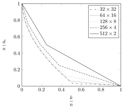
Figure 2: Performance of the codes in Example 11

Below we investigate in detail how well general optimal weighted Reed-Muller codes ${\mbox{RM}}(S_{1},S_{2},u,w_{1},w_{2})$ perform in comparison with $q$-ary Reed-Muller codes ${\mbox{RM}}(S,S,u^{\prime},1,1)$. Here, we assume that $s_{1}s_{2}=s^{2}$. Recall, from Proposition 7 that the description of the weights used in the optimal weighted Reed-Muller codes involves three cases depending on the value of $u$. Choosing in the following without loss of generality $w_{1}=1$ we shall refer to $u\leq s_{1}-(s_{1}/s_{2})$ as region I, $s_{1}-(s_{1}/s_{2})\leq u\leq s_{1}-1$ as region II, and finally $s_{1}-1\leq u\leq(s_{1}-1)+w_{2}(s_{2}-1)$ as region III. Proposition 12, Proposition 13, and Proposition 14, respectively, takes care of region I, region II, and region III, respectively. In Proposition 12 we will to ease the analysis make the small restriction that $s_{2}\mid s_{1}$ and that $s_{1}\mid us_{2}$. Furthermore, in all three propositions we assume that $u$ is an integer. We stress that when such assumptions do not hold then the formulas to be presented are still very close to be true. What we will learn is that the codes ${\mbox{RM}}(S_{1},S_{2},u,w_{1}=1,w_{2})$ always outperform the codes ${\mbox{RM}}(S,S,u^{\prime},1,1)$ provided that $s_{1}\geq 4s_{2}$. Furthermore, for $s_{1}-s/s_{2}\leq u$ such a result holds in the general situation $s_{1}>s_{2}$.

Proposition 12.

Consider integers $s_{1},s_{2}$ with $1<s_{2}<s_{1}$. Let $u$ be an integer with $u\leq s_{1}-(s_{1}/s_{2})$. Assume $s_{1}/s_{2}$ and $us_{2}/s_{1}$ are integers and that $s_{1}s_{2}=s^{2}$ for some integer $s$. Let $w_{1}=1$ and $w_{2}=s_{1}/s_{2}$ (that is, $w_{1}$ and $w_{2}$ are chosen as in Proposition 7). The code ${\mbox{RM}}(S_{1},S_{2},u,w_{1},w_{2})$ is of dimension

$$\frac{1}{2}(u^{2}\frac{s_{2}}{s_{1}}+u)+u\frac{s_{2}}{s_{1}}+1$$

and any ${\mbox{RM}}(S,S,u^{\prime},1,1)$ of the same or larger minimum distance is of dimension at most

$$\frac{1}{2}(\frac{s_{2}}{s_{1}}u^{2}+3u\sqrt{\frac{s_{2}}{s_{1}}}+2).$$

For $s_{1}\geq 4s_{2}$ the code ${\mbox{RM}}(S_{1},S_{2},u,w_{1},w_{2})$ is the better one.

Proof.

The dimension of ${\mbox{RM}}(S_{1},S_{2},u,w_{1},w_{2})$ is

$$\sum_{i=1}^{us_{2}/s_{1}}\frac{i}{s_{1}}{s_{2}}+\frac{us_{2}}{s_{1}}+1$$

and the minimum distance is $s_{2}(s_{1}-u)$. Assuming $u^{\prime}=u\sqrt{\frac{s_{2}}{s_{1}}}$ is an integer, the code ${\mbox{RM}}(S,S,u^{\prime},1,1)$ is of minimum distance $s_{2}(s_{1}-u)$. This code is of dimension

$$\frac{1}{2}(\frac{s_{2}}{s_{1}}u^{2}+3u\sqrt{\frac{s_{2}}{s_{1}}}+2).$$

∎

Proposition 13.

Consider integers $s_{1}$ and $s_{2}$ with $s_{2}<s_{1}$. Let $u$ be an integer with

$$s_{1}-\frac{s_{1}}{s_{2}}\leq u\leq s_{1}-1.$$

Assume $s_{1}s_{2}=s^{2}$ for some integer $s$. Let $w_{1}=1$ and $w_{2}=s_{1}-u$ (that is, $w_{1}$ and $w_{2}$ are chosen as in Proposition 7). The dimension of ${\mbox{RM}}(S_{1},S_{2},u,w_{1},w_{2})$ equals

$$s_{1}s_{2}-\frac{s_{2}^{2}(s_{1}-u)}{2}+s_{2}-\frac{s_{2}(s_{1}-u)}{2}.$$ (15)

If $u\geq s_{1}-s/s_{2}$ then any code ${\mbox{RM}}(S,S,u^{\prime},1,1)$ of the same or larger minimum distance is of dimension at most

$$s_{1}s_{2}-\frac{(s_{1}-u)s_{2}((s_{1}-u)s_{2}-1)}{2}$$

which is less than (15) for $s_{2}<s_{1}$. If $u<s_{1}-s/s_{2}$ then any code ${\mbox{RM}}(S,S,u^{\prime\prime},1,1)$ of the same or larger minimum distance is of dimension at most

$$\frac{1}{2}\big{(}\frac{s_{2}u}{s}+2\big{)}\big{(}\frac{s_{2}u}{s}+1\big{)}.$$

This number is smaller than the value of (15) for $s_{1}>4s_{2}$ and equal if $s_{1}=4s_{2}$.

Proof.

Consider the first code which is of minimum distance $(s_{1}-u)s_{2}$. For $i_{2}=s_{2}-1$ the value $i_{1}$ such that $w_{1}i_{1}+w_{2}i_{2}=u$ is $i_{1}=u-(s_{2}-1)(s_{1}-u)$. Therefore the dimension equals

$$s_{2}(i_{1}+1)+\sum_{i=1}^{s_{2}-1}(s_{1}-u)i=s_{1}s_{2}-\frac{s_{2}^{2}(s_{1}-u)}{2}+s_{2}-\frac{s_{2}(s_{1}-u)}{2}.$$

If $(s_{1}-u)s_{2}\leq s\Leftrightarrow u\geq s_{1}-s/s_{2}$ then for $u^{\prime}=2s-1-s_{1}s_{2}+us_{2}$ the code ${\mbox{RM}}(S,S,u^{\prime},1,1)$ is of the same minimum distance. This code is of dimension

$$s^{2}-\sum_{i=1}^{(s_{1}-u)s_{2}-1}i=s_{1}s_{2}-\frac{(s_{1}-u)s_{2}((s_{1}-u)s_{2}-1)}{2}.$$

The dimension of the first code exceed the dimension of the latter code by $(s_{1}-u-1)\big{(}s_{2}^{2}(s_{1}-u)/2-s_{2}\big{)}$ which is a positive number for $u<s_{1}-1$ and equals zero for $u=s_{1}-1$.
If $(s_{1}-u)s_{2}>s\Leftrightarrow u<s_{1}-s/s_{2}$ then imagining that $s$ divides $s_{2}(s_{1}-u)$ the code ${\mbox{RM}}(S,S,u^{\prime\prime},1,1)$ with

$$(s-u^{\prime\prime})s=s_{2}(s_{1}-u)\Leftrightarrow u^{\prime\prime}=\frac{us_{2}}{s}$$

is of the same minimum distance as ${\mbox{RM}}(S_{1},S_{2},u,w_{1},w_{2})$. The dimension equals

$$\sum_{i=1}^{u^{\prime\prime}+1}i=\frac{1}{2}\big{(}\frac{s_{2}u}{s}+2\big{)}\big{(}\frac{s_{2}u}{s}+1\big{)}.$$

Subtracting this expression from (15) one gets a concave function (a parabola) in $u$. Therefore the smallest value of the difference is attained either for $u=s_{1}-s_{1}/s_{2}$ or for $u=s_{1}-s/s_{2}$. Plugging in the first value and substituting $s_{1}=xs$, $s_{2}=s/x$ one finds that the resulting function is zero for $x=2$ and positive for $x\in]2;s[$. Plugging in the latter value is not needed as we already know from the first part of the theorem that here the difference is positive. ∎

Proposition 14.

Consider integers $s_{1}$ and $s_{2}$ with $1<s_{2}<s_{1}$ and $s_{1}s_{2}=s^{2}$ where $s$ is an integer. Let $u$ be an integer with $s_{1}-1\leq u\leq(s_{1}-1)+(s_{2}-1)$. Let $w_{1}=w_{2}=1$ (that is, $w_{1}$ and $w_{2}$ are chosen as in Proposition 7). There is a Reed-Muller code over $S\times S$ of the same minimum distance and the same dimension.

Example 15.

This is a continuation of Example 11. Consider the graph in Figure 2. First we take a look at the optimal weighted Reed-Muller codes corresponding to $(s_{1},s_{2})=(64,16)$. For these codes region I (Proposition 12) corresponds to rates $k/n$ below approximately $0.5$. As $64=4\cdot 16$ we expect the optimal weighted Reed-Muller codes to behave very much like the corresponding Reed-Muller codes in this region, which is indeed what the graph reveals. Considering values of $(s_{1},s_{2})$ with $s_{1}>4s_{2}$, when $s_{1}/s_{2}$ increases the rates corresponding to region I defines a smaller and smaller interval (starting of course still with rate equal to 0). The improvements in region I increases, but a more important contribution for the codes to become better and better is that region II takes over at smaller rates. Similarly, the interval of rates corresponding to region III (Proposition 14) becomes smaller and smaller. This is the interval where the optimal weighted Reed-Muller codes are (again) as bad as the $q$-ary Reed-Muller codes. For $(s_{1},s_{2})=(64,16)$ this last mentioned interval starts at approximately $0.875$. Already for $(s_{1},s_{2})=(128,8)$ the starting point of the interval is around $0.97$.

Proposition 12, Proposition 13 and Proposition 14 tell us that whenever $s_{1}\geq 4s_{2}$ then the optimal weighted Reed-Muller codes outperform the Reed-Muller codes coming from $S\times S$. Example 11 further suggests that from that point further increasing $s_{1}$ and decreasing $s_{2}$ can only help. The following three propositions together confirm this observation. As in previous propositions we will need to make a few assumptions on the codes that we consider. Again we stress that when such assumptions do not hold then the formulas to be presented are still very close to be true.

Proposition 16.

Consider positive integers $s_{1},s_{2},s_{1}^{\prime},s_{2}^{\prime}$ with $s_{1}s_{2}=s_{1}^{\prime}s_{2}^{\prime}$, $s_{1}^{\prime}>s_{1}>s_{2}>s_{2}^{\prime}$ and $s_{1}/s_{2}\geq 2$. Let $u$, $0<u\leq s_{1}-s_{1}/s_{2}$ be an integer with $s_{1}|us_{2}$ and consider the optimal weighted Reed-Muller code

$${\mbox{RM}}(S_{1},S_{2},u,w_{1}=1,w_{2}=s_{1}/s_{2}).$$ (16)

If for an integer $u^{\prime}$ with $s_{1}^{\prime}|u^{\prime}s_{2}^{\prime}$ ${\mbox{RM}}(S_{1}^{\prime},S_{2}^{\prime},u^{\prime},w_{1}^{\prime},w_{2}^{\prime})$ is an optimal weighted Reed-Muller code of the same or smaller minimum distance as that of (16) then the latter code is of dimension at least that of the first one.

Proof.

If the latter code is of minimum distance close to that of (16) then it belongs to region I or II. The codes are of minimum distance $d=s_{2}(s_{1}-u)$ and $d^{\prime}=s_{2}^{\prime}(s_{1}^{\prime}-u^{\prime})$, respectively. Hence, $u^{\prime}\geq us_{2}/s_{2}^{\prime}$. If the latter code is in region I the improvement in dimension is at least

$$-u(\frac{1}{2}+\frac{s_{2}}{s_{1}}-\frac{s_{2}}{2s_{2}^{\prime}}-\frac{s_{2}}{s_{1}^{\prime}})$$

which is positive when $s_{2}+s_{1}/2<s_{2}^{\prime}+s_{1}^{\prime}/2$. Writing $s_{1}^{\prime}=\mu s_{1}$ this corresponds to

$$\mu^{2}(s_{1}/2)+\mu(-s_{2}-s_{1}/2)+s_{2}>0.$$ (17)

The left side is a convex parabola with roots $\mu=1$ and $\mu=2s_{2}/s_{1}$. The assumption $s_{1}/s_{2}\geq 2$ therefore guarantees that (17) holds for all $\mu>1$.
Assume next that the latter code in the proposition is in region II. The improvement can be calculated to be

$$u^{2}(-\frac{s_{2}}{2s_{1}})+u(\frac{s_{2}s_{2}^{\prime}}{2}+\frac{s_{2}}{2}-\frac{s_{2}}{2s_{1}})+(\frac{s_{1}s_{2}}{2}-\frac{s_{2}^{\prime}s_{1}s_{2}}{2}+s_{2}^{\prime}-1)$$ (18)

which is a concave function in $u$. Our assumptions give $s_{1}-s_{1}/s_{2}^{\prime}\leq u\leq s_{1}-s_{1}/s_{2}$ and therefore it is enough to plug $u=s_{1}-s_{1}/s_{2}^{\prime}$ and $u=s_{1}-s_{1}/s$ into (18) and then to check that the resulting values are positive. The first value is positive if

$$\mu^{3}(-\frac{s_{1}}{2s_{2}})+\mu^{2}(1+\frac{s_{1}}{2s_{2}}+\frac{s_{1}}{2})+\mu(-1-\frac{s_{1}}{2}-s_{2})+s_{2}$$ (19)

is positive. The roots of this function in $\mu$ are $0$, $2s_{2}/s_{1}$, and $s_{2}$. Hence, (19) is indeed positive for $\mu\in]1,s_{2}[$. When $u=s_{1}-s_{1}/s_{2}$ is plugged into (18) we get

$$\frac{s_{2}}{\mu}+\frac{s_{1}s_{2}}{2}-s_{2}-\frac{s_{1}s_{2}}{2\mu}$$

which is positive for $\mu>1$. ∎

Proposition 17.

Consider positive integers $s_{1},s_{2},s_{1}^{\prime},s_{2}^{\prime}$ with $s_{1}s_{2}=s_{1}^{\prime}s_{2}^{\prime}$, $s_{1}^{\prime}>s_{1}>s_{2}>s_{2}^{\prime}$, and $s_{1}/s_{2}\geq 2$. Let $u$, $s_{1}-s_{1}/s_{2}\leq u\leq s_{1}-1$ be an integer and consider the optimal weighted Reed-Muller code

$${\mbox{RM}}(S_{1},S_{2},u,w_{1}=1,w_{2}=s_{1}-u).$$ (20)

If for an integer $u^{\prime}$ ${\mbox{RM}}(S_{1}^{\prime},S_{2}^{\prime},u^{\prime},w_{1}^{\prime},w_{2}^{\prime})$ is an optimal weighted Reed-Muller code of the same or smaller minimum distance as that of (20) then the latter code is of dimension at least that of the first one.

Proof.

If the latter code is of minimum distance close to that of (20) then it belongs to region II. As in the proof of the preceding proposition we have $u^{\prime}\geq us_{2}/s_{2}^{\prime}$. The improvement in dimension can be calculated to be at least

$$(s_{2}-s_{2}^{\prime})(\frac{s_{1}s_{2}}{2}-\frac{s_{2}u}{2}-1)$$

which takes on its minimal value $s_{2}/2-1$ for $u=s_{1}-1$. Combining this with the assumption $s_{2}>s_{2}^{\prime}\geq 1$ proves the proposition. ∎

Proposition 18.

Consider positive integers $s_{1},s_{2},s_{1}^{\prime},s_{2}^{\prime}$ with $s_{1}s_{2}=s_{1}^{\prime}s_{2}^{\prime}$, $s_{1}^{\prime}>s_{1}>s_{2}>s_{2}^{\prime}$. Let $u$, $s_{1}-1\leq u\leq(s_{1}-1)+(s_{2}-1)$ be an integer and consider the optimal weighted Reed-Muller code

$${\mbox{RM}}(S_{1},S_{2},u,w_{1}=1,w_{2}=1).$$ (21)

If for an integer $u^{\prime}$ ${\mbox{RM}}(S_{1}^{\prime},S_{2}^{\prime},u^{\prime},w_{1}^{\prime}=1,w_{2}^{\prime})$ is an optimal weighted Reed-Muller code of the same or smaller minimum distance as that of (21) then the latter code is of dimension at least that of the first one.

Proof.

The latter code either belongs to region II or III. For those in region III the result is pretty obvious so we consider only codes in region II. Let $d$ be the minimum distance of the code in (21). We have $u^{\prime}\geq(s_{1}s_{2}-d)/s_{2}^{\prime}$. The improvement in dimension can be calculated to be at least

$$\frac{1}{2}d^{2}+d(-1-\frac{s_{2}^{\prime}}{2})+s_{2}^{\prime}.$$

We may assume $d>s_{2}^{\prime}$ as we are in region II and the result follows. ∎

The construction of weighted Reed-Muller codes is very concrete, but for completeness we should mention that it is not the most optimal. Consider instead the codes $E({\mathbb{M}},{\mathcal{S}})$ with ${\mathcal{S}}=S_{1}\times\cdots\times S_{m}$ and

$${\mathbb{M}}=\{X_{1}^{i_{1}}\cdots X_{m}^{i_{m}}\mid(s_{1}-i_{1})\cdots(s_{m}-i_{m})\geq\delta\}.$$ (22)

Among the codes with designed distance $\delta$ (Theorem 4) these are the codes of highest possible dimension. When $S_{1}=\cdots=S_{m}={\mathbf{F}}_{q}$ holds the construction simply is that of Massey-Costello-Justesen codes (see [20] and [16]).

4 Dual codes

As is well-known, for the special case of ${\mathcal{S}}={\mathbf{F}}_{q}\times\cdots\times{\mathbf{F}}_{q}$ the duals of $q$-ary Reed-Muller codes, weighted Reed-Muller codes, and Massey-Costello-Justesen codes, respectively, are $q$-ary Reed-Muller codes, weighted Reed-Muller codes, and hyperbolic codes, respectively [28], [9] (for the definition of hyperbolic codes we refer to (24) below). More examples of codes $E({\mathbb{M}},{\mathcal{S}})$ where similar neat correspondences hold can be found in [4]. Turning to a general point ensemble ${\mathcal{S}}=S_{1}\times\cdots\times S_{m}$, however, it does not in general hold that the dual of a weighted Reed-Muller code is again a weighted Reed-Muller code. Nor does it hold in general that the dual of a Massey-Costello-Justesen code is a hyperbolic code. For a simple counter example which fits the description of a weighted Reed-Muller code as well as the description of a Massey-Costello-Justesen code consider the ordinary Reed-Solomon code over ${\mathcal{S}}=\mathbf{F}_{q}^{\ast}$ and recall that ${\mbox{ev}}_{\mathcal{S}}(1)$ is not a parity check for this particular code.
Fortunately, for the class of codes

$$E^{\perp}({\mathbb{M}},\mathcal{S}) =\{\vec{c}\in{\mathbf{F}}_{q}^{n=|\mathcal{S}|}\mid\vec{c}\cdot{\mbox{ev}}_{\mathcal{S}}(M)=0,{\mbox{ for all }}M\in{\mathbb{M}}\}$$

we have a technique similar to that of Section 2 to estimate the minimum distance. This technique is known as the Feng-Rao bound ([7], [8]). We now recall this bound following the description of Shibuya and Sakaniwa in [27]. Consider the following definition of a linear code.

Definition 19.

Let $B=\{{\vec{b}}_{1},\ldots,{\vec{b}}_{n}\}$ be a basis for ${\mathbf{F}}_{q}^{n}$ and let $G\subseteq B$. We define $C(B,G)={\mbox{Span}}_{\mathbf{F}_{q}}\{\vec{b}\mid\vec{b}\in G\}$. The dual code is denoted $C^{\perp}(B,G)$.

The Feng-Rao bound calls for the following set of spaces.

Definition 20.

Let $L_{-1}=\emptyset$, $L_{0}=\{\vec{0}\}$ and $L_{l}={\mbox{Span}}_{\mathbf{F}_{q}}\{\vec{b}_{1},\ldots,\vec{b}_{l}\}$ for $l=1,\ldots,n$.

We obviously have a chain of spaces $\{\vec{0}\}=L_{0}\subsetneq L_{1}\subsetneq\cdots\subsetneq L_{n-1}\subsetneq L_{n}={\mathbf{F}}_{q}^{n}$. Hence, we can define a function as follows.

Definition 21.

Define $\bar{\rho}:{\mathbf{F}}_{q}^{n}\rightarrow\{0,1,\ldots,n\}$ by $\bar{\rho}(\vec{v})=l$ if $\vec{v}\in L_{l}\backslash L_{l-1}$.

Definition 22.

Let $I=\{1,2,\ldots,n\}$. An ordered pair $(i,j)\in I^{2}$ is said to be well-behaving if $\bar{\rho}(\vec{b}_{u}\ast\vec{b}_{v})<\bar{\rho}(\vec{b}_{i}\ast\vec{b}_{j})$ for all $u$ and $v$ with $1\leq u\leq i,1\leq v\leq j$ and $(u,v)\neq(i,j)$. Here, $\ast$ is the componentwise product.

Definition 23.

For $l=1,\ldots,n$ define

$$\bar{\mu}(l)=\#\{(i,j)\in I^{2}\mid(i,j){\mbox{ is well-behaving and }}\bar{\rho}(\vec{b}_{i}\ast\vec{b}_{j})=l\}.$$

The Feng-Rao bound now is ([27, Prop. 1]):

Theorem 24.

The minimum distance of $C^{\perp}(B,G)$ is at least

$$\min\{\bar{\mu}(l)\mid\vec{b}_{l}\notin G\}.$$

Turning to the codes $E(\mathbb{M},\mathcal{S})$ we enumerate the basis

$$\{{\mbox{ev}}_{\mathcal{S}}(X_{1}^{i_{1}}\cdots X_{m}^{i_{m}})\mid 0\leq i_{1}<s_{1},\ldots,0\leq i_{m}<s_{m}\}$$

according to a total degree lexicographic ordering on the monomials $X_{1}^{i_{1}}\cdots X_{m}^{i_{m}}$. For ${\vec{b}}_{l}={\mbox{ev}}_{\mathcal{S}}(X_{1}^{i_{1}}\cdots X_{m}^{i_{m}})$, $0\leq i_{1}<s_{1},\ldots,0\leq i_{m}<s_{m}$, we clearly have $\bar{\mu}(l)\geq(i_{1}+1)\cdots(i_{m}+1)$. Hence, by the Feng-Rao bound the minimum distance of $E^{\perp}({\mathbb{M}},\mathcal{S})$ is at least

$$\min\{(i_{1}+1)\cdots(i_{m}+1)\mid X_{1}^{i_{1}}\cdots X_{m}^{i_{m}}\notin{\mathbb{M}},0\leq i_{1}<s_{1},\ldots,0\leq i_{m}<s_{m}\}.$$ (23)

Consider the code

$$({\mbox{RM}}(S_{1},\ldots,S_{m},(s_{1}-1)\cdots(s_{m}-1)-u-\epsilon,w_{1},\ldots,w_{m}))^{\perp}$$

where $\epsilon$ is a very small positive number. The bound (23) tells us that the minimum distance is at least that of the weighted Reed-Muller code ${\mbox{RM}}(S_{1},\ldots,S_{m},$ $u,w_{1},\ldots,w_{m})$. Observe that the codes are of the same dimension. Similarly, the hyperbolic code $E^{\perp}({\mathbb{M}},\mathcal{S})$

$$\mathbb{M} = \{X_{1}^{i_{1}}\cdots X_{m}^{i_{m}}\mid(i_{1}+1)\cdots(i_{m}+1)<\delta\}$$ (24)

has designed minimum distance equal to $\delta$ just as the Massey-Costello-Justesen code in (22). Again, the two codes are of the same dimension.
The Feng-Rao bound comes with a decoding algorithm that corrects up to half the designed minimum distance [8, 14]. This algorithm of course applies in particular to the above dual codes.
The remaining part of the paper is concerned with decoding algorithms for the codes $E({\mathbb{M}},\mathcal{S})$ including the codes from Section 3.

5 Subfield subcode decoding

As already noted by Kasami et al. in [17], any ordinary $q$-ary Reed-Muller code (in the terminology of the present paper this means a $q$-ary Reed-Muller code from ${\mathcal{S}}={\mathbf{F}}_{q}\times\cdots\times{\mathbf{F}}_{q}$) can be seen as a subfield subcode of a Reed-Solomon code. The Reed-Solomon code will be over the field ${\mathbf{F}}_{q^{m}}$ and is constructed by evaluating polynomials of degree at most $uq^{m-1}$ in the $q^{m}$ different elements of ${\mathbf{F}}_{q^{m}}$. The above observation guarantees that codes $E({\mathbb{M}},\mathcal{S})$ in general can be seen as subcodes of subfield subcodes of certain Reed-Solomon codes over ${\mathbf{F}}_{q^{m}}$, but it is not straightforward which elements of ${\mathbf{F}}_{q^{m}}$ to use. This problem, however, is easy to overcome if we use the approach by Santhi [25].
Let $\{\vec{b}_{1},\ldots,\vec{b}_{n}\}$ be a basis for ${\mathbb{F}}_{q^{m}}$ as a vectorspace over ${\mathbf{F}}_{q}$. Following Santhi we now define a map $\varphi:{\mathbb{F}}_{q}^{m}\rightarrow{\mathbb{F}}_{q^{m}}$ by

$$\varphi(a_{1},\ldots,a_{m})=a_{1}\vec{b}_{1}+\cdots+a_{m}\vec{b}_{m}$$ (25)

and note that $\varphi(a_{1},\ldots,a_{m})^{q^{v}}=a_{1}\vec{b}_{1}^{q^{v}}+\cdots+a_{m}\vec{b}_{m}^{q^{v}}$. Writing $X=\varphi(a_{1},\ldots,a_{m})$ we have

$$\left[\begin{array}[]{ccc}\vec{b}_{1}&\cdots&\vec{b}_{m}\\ \vec{b}_{1}^{q}&\cdots&\vec{b}_{m}^{q}\\ \vdots&\ddots&\vdots\\ \vec{b}_{1}^{q^{m-1}}&\cdots&\vec{b}_{m}^{q^{m-1}}\end{array}\right]\left[\begin{array}[]{c}a_{1}\\ a_{2}\\ \vdots\\ a_{m}\end{array}\right]=\left[\begin{array}[]{c}X\\ X^{q}\\ \vdots\\ X^{q^{m-1}}\end{array}\right].$$

By [19, Cor. 2.38] the matrix on the left side is invertible and therefore there exist polynomials $F_{1},\ldots,F_{m}\in{\mathbb{F}}_{q^{m}}[T]$ such that $a_{i}=F_{i}(X)$. The polynomials $F_{1},\ldots,F_{m}$ do not depend on the point $(a_{1},\ldots,a_{m})$ under consideration. From this observation one deduces that $F(P)=F(F_{1}(\varphi(P)),\ldots,F_{m}(\varphi(P)))$ for all $P\in{\mathbb{F}}_{q}^{m}$.

Theorem 25.

Write ${\mathcal{S}}=\{P_{1},\ldots,P_{n}\}$. The code $E({\mathbb{M}},{\mathcal{S}})$ is a subcode of a subfield subcode of the Reed-Solomon code over ${\mathbf{F}}_{q^{m}}$ which is constructed by evaluating polynomials of degree at most

$$t=\max\{\deg M\mid M\in{\mathbb{M}}\}$$ (26)

in the elements $\varphi(P_{1}),\ldots,\varphi(P_{n})$. Here $\varphi$ is the function in (25).

Following the Pellikaan-Wu approach [21] we can now decode $E({\mathbb{M}},{\mathcal{S}})$ by applying the Guruswami-Sudan list decoding algorithm to the corresponding Reed-Solomon code [12] and by performing a few additional steps. The complexity of the Guruswami-Sudan list decoding algorithm is in the literature often claimed to be ${\mathcal{O}}(n^{3})$. For more precise statements of the decoding complexity which takes the multiplicity into account we refer to [3]. The Guruswami-Sudan algorithm corrects up to $n(1-\sqrt{R})$ errors of the Reed-Solomon code. It is therefore clear that the above approach can decode up to

$$\lceil n(1-\sqrt{\frac{tq^{m-1}+1}{n}})\rceil$$ (27)

errors of $E({\mathbb{M}},{\mathcal{S}})$ (Here, $t$ is as in (26)). This is indeed a fine result for many codes $E({\mathbb{M}},{\mathcal{S}})$. However, it is also clear that for other choices of $E({\mathbb{M}},{\mathcal{S}})$ (27) may be close to zero or even negative. For the particular case of an optimal weighted Reed-Muller code ${\mbox{RM}}(S_{1},S_{2},u,w_{1}=1,w_{2})$ (27) becomes

$$\lceil s_{1}s_{2}\big{(}1-\sqrt{\frac{uq+1}{s_{1}s_{2}}}\big{)}\rceil.$$ (28)

(recall from Proposition 7 that $w_{1}\leq w_{2}$ always holds). If $s_{1}s_{2}$ is close to $q^{2}$ and $u$ is not too large then this bound guarantees list decoding. If $s_{2}$ is much smaller than $s_{1}$ then the bound may not even guarantee that the algorithm can correct a single error. This is the reason why we in the present paper consider also a second decoding algorithm. Before getting to the second algorithm, we apply the first one to the Joyner code.

5.1 The Joyner code

Toric codes were introduced by Hansen in [13] and further generalized by Joyner in [15], by Ruano in [23, 24] and by Little et al.  in [18]. Among the most famous toric codes is the $[49,11,28]$ code over ${\mathbf{F}}_{8}$ presented in [15, Ex. 3.9]. This code is known as the Joyner code. Attempts have been made to decode it, but without much luck so far. We now demonstrate how to decode it even beyond its minimum distance by applying the method of this section in combination with a small trick.
The Joyner code originally was introduced in the language of polytopes. Alternatively, one can define it [24] as a code $E({\mathbb{M}},S)$ where

$${\mathcal{S}}={\mathbf{F}}_{8}^{\ast}\times{\mathbf{F}}_{8}^{\ast}=\{(x_{1},y_{1}),\ldots,(x_{49},y_{49})\},$$

$${\mathbb{M}}=\{1\}\cup\{X^{i}Y^{j}\mid 1\leq i,j{\mbox{ \ and \ }}i+j\leq 5\}.$$

Let the polynomial corresponding to a given code word $\vec{c}$ be

$$F(X,Y)=F_{0,0}+\sum_{\begin{array}[]{c}i,j\geq 1\\ i+j\leq 5\end{array}}F_{i,j}X^{i}Y^{j}.$$

Let $\vec{r}=\vec{c}+\vec{e}$ be the received word. Assume for a moment that we know $F_{0,0}$. We then subtract $(F_{0,0},\ldots,F_{0,0})$ from $\vec{r}$ to get a word $\vec{r^{\prime}}$ that in the error free positions corresponds to

$$\sum_{\begin{array}[]{c}i,j\geq 1\\ i+j\leq 5\end{array}}F_{i,j}X^{i}Y^{j}.$$

For $i=1,\ldots,49$ we now divide the $i$th entry of $\vec{r^{\prime}}$ with $x_{i}y_{i}$ to produce a word $\vec{r^{\prime\prime}}$. Observe, that this is doable because $x_{i},y_{i}\neq 0$ holds. The word $\vec{r^{\prime\prime}}$ in the error free positions corresponds to

$$\sum_{\begin{array}[]{c}i,j\geq 1\\ i+j\leq 5\end{array}}F_{i,j}X^{i-1}Y^{j-1}.$$

We have $\vec{r^{\prime\prime}}=\vec{c^{\prime\prime}}+\vec{e^{\prime\prime}}$ where $\vec{c^{\prime\prime}}\in E({\mathbb{M^{\prime\prime}}},{\mathcal{S}})$, ${\mathbb{M^{\prime\prime}}}=\{X^{i}Y^{j}\mid i+j\leq 3\}$ and $\vec{e^{\prime\prime}}$ is non-zero in exactly the same positions as $\vec{e}$. The Reed-Muller code $E(\mathbb{M^{\prime\prime}},{\mathcal{S}})$ is a subfield subcode of a $[49,25,25]$ Reed-Solomon code over ${\mathbf{F}}_{64}$. The exact form of the Reed-Solomon code is described by Theorem 25. Given a code word from the output of the Reed-Solomon list decoder we multiply for $i=1,\ldots,49$ the $i$th entry with $x_{i}y_{i}$ and add $F_{0,0}$.
Of course we do not as assumed above know $F_{0,0}$ in advance. Therefore we must try out all $8$ possible values of this number. The error correction capability of the corresponding algorithm is described in Table 1. We see that we can correct up to $31$ errors even though the minimum distance of the Joyner code is only $28$.

Table 1: Error correction capability when the multiplicity used of the Reed-Solomon code decoder is $m$

$m$	1	2	3	4	5	6
capability	12	20	24	27	29	31

6 An interpretation of the Guruswami-Sudan list decoding algorithm

The second decoding algorithm of the present paper is a direct interpretation of the Guruswami-Sudan list decoding algorithm. We build on works by Pellikaan et al. [21], and Augot et al. [1], [2] who concentrated on $q$-ary Reed-Muller codes and Reed-Solomon product codes. We consider general code $E({\mathbb{M}},{\mathcal{S}})$ and improve on the above mentioned work by establishing new information on how many zeros of prescribed multiplicity a polynomial can have when given information about its leading monomial with respect to the lexicographic ordering. In combination with a preparation step this will allow us to correct more errors. The idea of a preparation step comes from [10]. The improved information regarding the zeros is derived by strengthening results reported by Dvir et al. in [6]. This is done in Subsection 6.1. In Subsection 6.2 we present the algorithm and elaborate on its decoding radius.

6.1 Bounding the number of zeros of multiplicity $r$

The definition of multiplicity that we will use relies on the Hasse derivative. Before recalling the definition of the Hasse derivative let us fix some notation. Assume we have a vector of variables $\vec{X}=(X_{1},\ldots,X_{m})$ and a vector $\vec{k}=(k_{1},\ldots,k_{m})\in{\mathbf{N}}_{0}^{m}$ then we will write $\vec{X}^{\vec{k}}=X_{1}^{k_{1}}\cdots X_{m}^{k_{m}}$. In the following ${\mathbf{F}}$ is any field.

Definition 26.

Given $F(\vec{X})\in{\mathbf{F}}[\vec{X}]$ and $\vec{k}\in{\mathbf{N}}_{0}^{m}$ the $\vec{k}$’th Hasse derivative of $F$, denoted by $F^{(\vec{k})}(\vec{X})$ is the coefficient of $\vec{Z}^{\vec{k}}$ in $F(\vec{X}+\vec{Z})$. In other words

$$F(\vec{X}+\vec{Z})=\sum_{\vec{k}}F^{(\vec{k})}(\vec{X})\vec{Z}^{\vec{k}}.$$

The concept of multiplicity for univariate polynomials is generalized to multivariate polynomials in the following way.

Definition 27.

For $F(\vec{X})\in{\mathbf{F}}[\vec{X}]\backslash\{{0}\}$ and $\vec{a}\in{\mathbf{F}}^{m}$ we define the multiplicity of $F$ at $\vec{a}$ denoted by ${\mbox{mult}}(F,\vec{a})$ as follows: Let $M$ be an integer such that for every $\vec{k}=(k_{1},\ldots,k_{m})\in{\mathbf{N}}_{0}^{m}$ with $k_{1}+\cdots+k_{m}<M$, $F^{(\vec{k})}(\vec{a})=0$ holds, but for some $\vec{k}=(k_{1},\ldots,k_{m})\in{\mathbf{N}}_{0}^{m}$ with $k_{1}+\cdots+k_{m}=M$, $F^{(\vec{k})}(\vec{a})\neq 0$ holds, then ${\mbox{mult}}(F,\vec{a})=M$. If $F=0$ then we define ${\mbox{mult}}(F,\vec{a})=\infty$.

The Schwartz-Zippel bound with multiplicity was reported already in [1], [2] but was only recently proved,  [6]. It goes as follows:

Theorem 28.

Let $F(\vec{X})\in{\mathbf{F}}[\vec{X}]$ be a non-zero polynomial of total degree $u$. Then for any finite set $S\subseteq{\mathbf{F}}$

$$\sum_{\vec{a}\in S^{m}}{\mbox{mult}}(F,\vec{a})\leq u|S|^{{m-1}}.$$

We have the following useful corollary:

Corollary 29.

Let $F(\vec{X})\in{\mathbf{F}}[\vec{X}]$ be a non-zero polynomial of total degree $u$ and let $S\subseteq{\mathbf{F}}$ be finite. The number of zeros of $F$ of multiplicity at least $r$ from $S^{m}$ is at most

$$\frac{u}{r}|S|^{m-1}.$$ (29)

For the $q$-ary Reed-Muller codes

$${\mbox{RM}}_{q}(u,m)={\mbox{RM}}({\mathbf{F}}_{q},\ldots,{\mathbf{F}}_{q},u,1,\ldots,1),$$

Pellikaan and Wu in [21] presented two decoding algorithms, a subfield subcode decoding algorithm and a direct interpretation of the Guruswami-Sudan algorithm. The analysis of the latter relies on [22, Lem. 2.4, Lem. 2.5] which combines to the following result:

Proposition 30.

Consider a polynomial $F(\vec{X})\in{\mathbf{F}}[\vec{X}]$ of total degree $u$, $u<rq$ and define $w=\lfloor u/q\rfloor$. The number of points in ${\mathbf{F}}_{q}^{m}$ where $F$ has at least multiplicity $r$ is at most equal to

$$\frac{{m+r-1\choose m}q^{m}+(u-qw){m+r-w-2\choose m-1}q^{m-1}-{m+r-w-1\choose m}q^{m}}{{m+r-1\choose r-1}}.$$ (30)

Augot and Stepanov [1] gave an improved estimate on the decoding radius of the latter algorithm (the direct interpretation of the Gurswami-Sudan algorithm) by using instead Corollary 29. We here present a direct proof that indeed, Corollary 29 is stronger than Proposition 30.

Proposition 31.

For all $u\in[0,rq-1]$ it hold that (29) is smaller than or equal to (30).

Proof.

We consider the two expressions as functions in $u$ on the interval $[0,rq]$. Our first observation is that (30) is a continuously piecewise linear function, each piece corresponding to a particular value of $w$. The corresponding $r$ slopes constitute a decreasing sequence. Combining this observation with the fact that (29) is linear in $u$ and with the fact that the two expressions are the same at each of the end points of the interval proves the result. ∎

As a preparation step to improve upon Theorem 28 and Corollary 29 we start by generalizing them. We will need a couple of results from [6, Sec. 2]. The first corresponds to [6, Lem. 5].

Lemma 32.

Consider $F(\vec{X})\in{\mathbf{F}}[\vec{X}]$ and $\vec{a}\in{\mathbf{F}}^{m}$. For any $\vec{k}=(k_{1},\ldots,k_{m})\in{\mathbf{N}}_{0}^{m}$ we have

$${\mbox{mult}}(F^{(\vec{k})},\vec{a})\geq mult(F,\vec{a})-(k_{1}+\cdots+k_{m}).$$

The next result that we recall corresponds to the last part of [6, Proposition 6].

Proposition 33.

Given $F(X_{1},\ldots,X_{m})\in{\mathbf{F}}[X_{1},\ldots,X_{m}]$ and

$$Q(Y_{1},\ldots,Y_{l})=(Q_{1}(\vec{Y}),\ldots,Q_{m}(\vec{Y}))\in{\mathbf{F}}[Y_{1},\ldots,Y_{l}]^{m}$$

let $F\circ Q$ be the polynomial $F(Q_{1}(\vec{Y}),\ldots,Q_{m}(\vec{Y}))$. For any $\vec{a}\in{\mathbf{F}}^{l}$ we have

$${\mbox{mult}}(F\circ Q,\vec{a})\geq{\mbox{mult}}(F,Q(\vec{a})).$$

We get the following Corollary, which is closely related to [6, Corollary 7].

Corollary 34.

Let $F(X_{1},\ldots,X_{m})\in{\mathbf{F}}[X_{1},\ldots,X_{m}]$ and $\vec{b}_{1},\ldots,\vec{b}_{m-1},\vec{c}\in{\mathbf{F}}^{m}$ be given. Write $F^{\ast}(T_{1},\ldots,T_{m-1})=F(T_{1}\vec{b}_{1}+\cdots+T_{m-1}\vec{b}_{m-1}+\vec{c})$. For any $(t_{1},\ldots,t_{m-1})\in{\mathbf{F}}^{m-1}$ we have

$${\mbox{mult}}(F^{\ast}(T_{1},\ldots,T_{m-1}),(t_{1},\ldots,t_{m-1}))\\ \geq{\mbox{mult}}(F(X_{1},\ldots,X_{m}),t_{1}\vec{b}_{1}+\cdots+t_{m-1}\vec{b}_{m-1}+\vec{c}).$$

Let $\prec$ be the lexicographic ordering on the set of monomials in variables $X_{1},\ldots,X_{m}$ such that $X_{m}\prec\cdots\prec X_{1}$ holds. We now write

$$F(X_{1},\ldots,X_{m})=\sum_{j_{1},\ldots,j_{m-1}}X_{1}^{j_{1}}\cdots X_{m-1}^{j_{m-1}}F_{j_{1},\ldots j_{m-1}}(X_{m}).$$

Let $X_{1}^{i_{1}}\cdots X_{m}^{i_{m}}$ be the leading monomial of $F$ with respect to $\prec$. Then due to the definition of $\prec$, $F_{i_{1},\ldots,i_{m-1}}(X_{m})$ is a (univariate) polynomial of degree $i_{m}$. For $a_{m}\in{\mathbf{F}}$ define

$$r(a_{m})={\mbox{mult}}(F_{i_{1},\ldots,i_{m-1}}(X_{m}),a_{m}).$$

Clearly,

$$\sum_{a_{m}\in S_{m}}r(a_{m})\leq i_{m}.$$ (31)

We have

$$F^{(0,\ldots,0,r(a_{m}))}(X_{1},\ldots,X_{m})=\sum_{j_{1},\ldots,j_{m-1}}X_{1}^{j_{1}}\cdots X_{m-1}^{j_{m-1}}F_{j_{1},\ldots,j_{m-1}}^{(r(a_{m}))}(X_{m})$$

and due to the definition of $\prec$ and to the definition of $r(a_{m})$ we have

$${\mbox{lm}}_{\prec}(F^{(0,\ldots,0,r(a_{m}))}(X_{1},\ldots,X_{m-1},a_{m}))=X_{1}^{i_{1}}\cdots X_{m-1}^{i_{m-1}}.$$ (32)

Applying first Lemma 32 with $\vec{k}=(0,\ldots,0,r(a_{m}))$ and afterwards Corollary 34 with $\vec{b}_{1}=(1,0,\ldots,0),\ldots,\vec{b}_{m-1}=(0,\ldots,0,1,0)$, $\vec{c}=(0,\ldots,0,a_{m})$ and $t_{1}=a_{1},\ldots,t_{m-1}=a_{m-1}$ we get the following result which is closely related to a result in [6, Proof of Lemma 8]:

$${\mbox{mult}}\big{(}F(X_{1},\ldots,X_{m}),(a_{1},\ldots,a_{m})\big{)}$$

$$\leq(0+\cdots+0+r(a_{m}))+{\mbox{mult}}\big{(}F^{(0,\ldots,0,r(a_{m}))}(X_{1},\ldots,X_{m}),(a_{1},\ldots,a_{m})\big{)}$$

$$\leq r(a_{m})+{\mbox{mult}}\big{(}F^{(0,\ldots,0,r(a_{m}))}(X_{1},\ldots,X_{m-1},a_{m}),(a_{1},\ldots,a_{m-1})\big{)}.$$ (33)

We are now ready to generalize Theorem 28. Let in the remaining part of this subsection $S_{1},\ldots,S_{m}$ be finite subsets of arbitrary field ${\mathbf{F}}$. Also we will relax from the assumption that $s_{1}\geq\cdots\geq s_{m}$.

Theorem 35.

Let $F(\vec{X})\in{\mathbf{F}}[\vec{X}]$ be a non-zero polynomial and let ${\mbox{lm}}(F)=X_{1}^{i_{1}}\cdots X_{m}^{i_{m}}$ be its leading monomial with respect to a lexicographic ordering. Then for any finite sets $S_{1},\ldots,S_{m}\subseteq{\mathbf{F}}$

$$\sum_{\vec{a}\in S_{1}\times\cdots\times S_{m}}{\mbox{mult}}(F,\vec{a})\leq i_{1}s_{2}\cdots s_{m}+s_{1}i_{2}s_{3}\cdots s_{m}+\cdots+s_{1}\cdots s_{m-1}i_{m}.$$

Proof.

We prove the theorem for the monomial ordering $\prec$. Dealing with general lexicographic orderings is simply a question of relabeling the variables. Clearly the theorem holds for $m=1$. For $m>1$ we consider (33). Assuming the theorem holds when the number of variables is smaller than $m$ we get by applying (31) and (32) the following estimate

$$\sum_{\vec{a}\in S_{1}\times\cdots\times S_{m}}{\mbox{mult}}(F,\vec{a})$$

$$\leq i_{m}s_{1}\cdots s_{m-1}+s_{m}(i_{1}s_{2}\cdots s_{m-1}+\cdots+i_{m-1}s_{1}\cdots s_{m-2})$$

$$=i_{1}s_{2}\cdots s_{m}+i_{2}s_{1}s_{3}\cdots s_{m}+\cdots i_{m}s_{1}\cdots s_{m-1}$$

as required. ∎

We have the following immediate generalization of Corollary 29.

Corollary 36.

Let $F(\vec{X})\in{\mathbf{F}}[\vec{X}]$ be a non-zero polynomial and let ${\mbox{lm}}(F)=X_{1}^{i_{1}}\cdots X_{m}^{i_{m}}$ be its leading monomial with respect to a lexicographic ordering. Assume $S_{1},\ldots,S_{m}\subseteq{\mathbf{F}}$ are finite sets. Then over $S_{1}\times\cdots\times S_{m}$ the number of zeros of multiplicity at least $r$ is less than or equal to

$$\big{(}i_{1}s_{2}\cdots s_{m}+s_{1}i_{2}s_{3}\cdots s_{m}+\cdots+s_{1}\cdots s_{m-1}i_{m}\big{)}/r.$$ (34)

The analysis leading to Theorem 28 suggests the following function to more accurately estimate the number of zeros of multiplicity at most $r$ of a polynomial with leading monomial $X_{1}^{i_{1}}\cdots X_{m}^{i_{m}}$:

Definition 37.

Let $r\in{\mathbf{N}},i_{1},\ldots,i_{m}\in{\mathbf{N}}_{0}$. Define

$$D(i_{1},r,s_{1})=\min\big{\{}\big{\lfloor}\frac{i_{1}}{r}\big{\rfloor},s_{1}\big{\}}$$

and for $m\geq 2$

$$D(i_{1},\ldots,i_{m},r,s_{1},\ldots,s_{m})=\\ \begin{split}\max_{(u_{1},\ldots,u_{r})\in A(i_{m},r,s_{m})}&\bigg{\{}(s_{m}-u_{1}-\cdots-u_{r})D(i_{1},\ldots,i_{m-1},r,s_{1},\ldots,s_{m-1})\\ &\quad+u_{1}D(i_{1},\ldots,i_{m-1},r-1,s_{1},\ldots,s_{m-1})+\cdots\\ &\quad+u_{r-1}D(i_{1},\ldots,i_{m-1},1,s_{1},\ldots,s_{m-1})+u_{r}s_{1}\cdots s_{m-1}\bigg{\}}\end{split}$$

where

$$A(i_{m},r,s_{m})=\\ \{(u_{1},\ldots,u_{r})\in{\mathbf{N}}_{0}^{r}\mid u_{1}+\cdots+u_{r}\leq s_{m}{\mbox{ \ and \ }}u_{1}+2u_{2}+\cdots+ru_{r}\leq i_{m}\}.$$ (35)

Theorem 38.

For a polynomial $F(\vec{X})\in{\mathbf{F}}[\vec{X}]$ let $X_{1}^{i_{1}}\cdots X_{m}^{i_{m}}$ be its leading monomial with respect to $\prec$ (this is the lexicographic ordering with $X_{m}\prec\cdots\prec X_{1}$). Then $F$ has at most $D(i_{1},\ldots,i_{m},r,s_{1},\ldots,s_{m})$ zeros of multiplicity at least $r$ in $S_{1}\times\cdots\times S_{m}$. The corresponding recursive algorithm produces a number that is at most equal to the number found in Corollary 36 and is at most equal to $s_{1}\cdots s_{m}$.

Proof.

The proof of the first part of the proposition is an induction proof. The result clearly holds for $m=1$. Given $m>1$ assume it holds for $m-1$. For $d=1,\ldots,r-1$ let $u_{d}$ be the number of $a_{m}$’s with $r(a_{m})=d$ and let $u_{r}$ be the number of $a_{m}$’s with $r(a_{m})\geq r$. The number of $a_{m}$’s with $r(a_{m})=0$ is $s_{m}-u_{1}-\cdots-u_{r}$. The boundary conditions that $u_{1}+\cdots+u_{r}\leq s_{m}$ and $u_{1}+2u_{2}+\cdots+ru_{r}\leq i_{m}$ are obvious. For every $a_{m}$ with $r(a_{m})=d$, $d=0,\ldots,r-1$ for $(a_{1},\ldots,a_{m})$ to be a zero of multiplicity at least $r$ the last expression in (33) must be at least $r-d$. For $a_{m}$ with $r(a_{m})\geq r$ all choices of $a_{1},\ldots,a_{m-1}$ are legal. This proves the first part of the proposition. As both Corollary 36 and the above proof rely on (33), Theorem 38 cannot produce a number greater than what is found in Corollary 36. The condition $u_{1}+\cdots+u_{r}\leq s_{m}$ and the definition of $D(i_{1},r,s_{1})$ imply the last result. ∎

It only makes sense to apply the function $D(i_{1},\ldots,i_{m},r,s_{1},\ldots,s_{m})$ to monomials $X_{1}^{i_{1}}\cdots X_{m}^{i_{m}}$ in

$$\Delta(r,s_{1},\ldots,s_{m})=\{X_{1}^{i_{1}}\cdots X_{m}^{i_{m}}\mid\lfloor i_{1}/s_{1}\rfloor+\cdots+\lfloor i_{m}/s_{m}\rfloor<r\}.$$

Proposition 39.

Assume $X_{1}^{i_{1}}\cdots X_{m}^{i_{m}}\notin\Delta(r,s_{1},\ldots,s_{m})$. Then there exists a polynomial with leading monomial $X_{1}^{i_{1}}\cdots X_{m}^{i_{m}}$ such that all elements of $S_{1}\times\cdots\times S_{m}$ are zeros of multiplicity at least $r$.

Example 40.

In a number of experiments listed in [11] we calculated the value $D(i_{1},\ldots,i_{m},r,q,\ldots,q)$ for various choices of $m$, $q$ and $r$ and for all values of $(i_{1},\ldots,i_{m})$ such that $X_{1}^{i_{m}}\cdots X_{m}^{i_{m}}\in\Delta(r,q,\ldots,q)$. Here we list the mean improvement in comparison with the situation where Corollary 29 is applied. More formally, we list in Table 2 for various fixed $q,r,m$ the mean value of

$$\frac{\min\{(i_{1}+\cdots+i_{m})q^{m-1}/r,q^{m}\}-D(i_{1},\ldots,i_{m},r,q,\ldots,q)}{\min\{(i_{1}+\cdots+i_{m})q^{m-1}/r,q^{m}\}}.$$ (36)

Table 2: The mean value of (36); truncated.

$m$		2								3								4
$r$		2		3		4		5		2		3		4		5		2		3
$q$	2	0.	363	0.	273	0.	337	0.	291	0.	301	0.	300	0.	342	0.	307	0.	248	0.	260
	3	0.	217	0.	286	0.	228	0.	236	0.	194	0.	224	0.	213	0.	214	0.	158	0.	177
	4	0.	191	0.	197	0.	232	0.	195	0.	158	0.	169	0.	180	0.	172	0.	125	0.	135
	5	0.	155	0.	167	0.	174	0.	197	0.	139	0.	145	0.	148	0.	153	0.	110	0.	116
	7	0.	128	0.	137	0.	138	0.	138	0.	119	0.	122	0.	121	0.	119	0.	093	0.	098
	8	0.	126	0.	127	0.	134	0.	126	0.	114	0.	115	0.	113	0.	111	0.	089	0.	093

Despite the significant mean improvement, according to our experiments in [11] for most fixed degrees $u$ there are examples of exponents $(i_{1},\ldots,i_{m})$, $i_{1}+\cdots+i_{m}=u$ such that $D(i_{1},\ldots,i_{m},r,s_{1},\ldots,s_{m})=\lfloor(i_{1}+\cdots+i_{m})q^{m-1}/r\rfloor$.

Sometimes the values $D(i_{1},\ldots,i_{m},r,s_{1},\ldots,s_{m})$ may be time consuming to calculate. Therefore it is relevant to have some closed formula estimates of these numbers. We next present such estimates for the case of two variables. Note, that the following proposition covers all monomials in $\Delta(r,s_{1},s_{2})$.

Proposition 41.

For $k=1,\ldots,r-1$, $D(i_{1},i_{2},r,s_{1},s_{2})$ is upper bounded by
$\begin{array}[]{cl}{\mbox{(C.1)}}&{\displaystyle{s_{2}\frac{i_{1}}{r}+\frac{i_{2}}{r}\frac{i_{1}}{r-k}}}\\ &{\mbox{if \ }}(r-k)\frac{r}{r+1}s_{1}\leq i_{1}<(r-k)s_{1}{\mbox{ \ and \ }}0\leq i_{2}<ks_{2},\\ {\mbox{(C.2)}}&{\displaystyle{s_{2}\frac{i_{1}}{r}+((k+1)s_{2}-i_{2})(\frac{i_{1}}{r-k}-\frac{i_{1}}{r})+(i_{2}-ks_{2})(s_{1}-\frac{i_{1}}{r})}}\\ &{\mbox{if \ }}(r-k)\frac{r}{r+1}s_{1}\leq i_{1}<(r-k)s_{1}{\mbox{ \ and \ }}ks_{2}\leq i_{2}<(k+1)s_{2},\\ {\mbox{(C.3)}}&{\displaystyle{s_{2}\frac{i_{1}}{r}+\frac{i_{2}}{k+1}(s_{1}-\frac{i_{1}}{r})}}\\ &{\mbox{if \ }}(r-k-1)s_{1}\leq i_{1}<(r-k)\frac{r}{r+1}s_{1}{\mbox{ \ and \ }}0\leq i_{2}<(k+1)s_{2}.\end{array}$
Finally,
$\begin{array}[]{cl}{\mbox{(C.4)}}&{\displaystyle{D(i_{1},i_{2},r,s_{1},s_{2})=s_{2}\lfloor\frac{i_{1}}{r}\rfloor+i_{2}(s_{1}-\lfloor\frac{i_{1}}{r}\rfloor)}}\\ &{\mbox{if \ }}s_{1}(r-1)\leq i_{1}<s_{1}r{\mbox{ \ and \ }}0\leq i_{2}<s_{2}.\end{array}$
The above numbers are at most equal to $\min\{(i_{1}s_{2}+s_{1}i_{2})/r,s_{1}s_{2}\}$.

Proof.

First we consider the values of $i_{1},i_{2},r,s_{1},s_{2}$ corresponding to one of the cases (C.1), (C.2), (C.3). Let $k$ be the largest number (as in Proposition 41) such that $i_{1}<(r-k)s_{1}$. Indeed $k\in\{1,\ldots,r-1\}$. We have

$$D(i_{1},i_{2},r,s_{1},s_{2})\leq\\ \max_{(u_{1},\ldots,u_{r})\in B(i_{2},r,s_{2})}\bigg{\{}s_{2}\frac{i_{1}}{r}+u_{1}(\frac{i_{1}}{r-1}-\frac{i_{1}}{r})+\cdots+u_{k}(\frac{i_{1}}{r-k}-\frac{i_{1}}{r})\\ +u_{k+1}(s_{1}-\frac{i_{1}}{r})+\cdots+u_{r}(s_{1}-\frac{i_{1}}{r})\bigg{\}}$$ (37)

where

$$B(i_{2},r,s_{2})=\{(u_{1},\ldots,u_{r})\in{\mathbf{Q}}^{r}\mid 0\leq u_{1},\ldots,u_{r},\\ u_{1}+\cdots+u_{r}\leq s_{2},u_{1}+2u_{2}+\cdots+ru_{r}\leq i_{2}\}.$$

We observe, that

$$k(\frac{i_{1}}{r-l}-\frac{i_{1}}{r})\leq l(\frac{i_{1}}{r-k}-\frac{i_{1}}{r})$$

holds for $l\leq k$. Furthermore, we have the biimplication

$$(r-k)\frac{r}{r+1}s_{1}\leq i_{1}\Leftrightarrow(k+1)(\frac{i_{1}}{r-k}-\frac{i_{1}}{r})\geq k(s_{1}-\frac{i_{1}}{r}).$$

Therefore, if the conditions in (C.1) are satisfied then (37) takes on its maximum when $u_{k}=\frac{i_{2}}{k}$ and the remaining $u_{i}$’s equal $0$. If the conditions in (C.2) are satisfied then (37) takes on its maximum at $u_{k}=(k+1)s_{2}-i_{2}$, $u_{k+1}=(i_{2}-ks_{2})$ and the remaining $u_{i}$’s equal $0$. If the conditions in (C.3) are satisfied then (37) takes on its maximal value at $u_{k+1}=\frac{i_{2}}{k+1}$ and the remaining $u_{i}$’s equal $0$.
Finally, if $s_{1}(r-1)\leq i_{1}<s_{1}r$ and $0\leq i_{2}\leq s_{2}$ then $D(i_{1},i_{2},r,s_{1},s_{2})$ is the maximal value of

$$s_{2}\lfloor\frac{i_{1}}{r}\rfloor+u_{1}(s_{1}-\lfloor\frac{i_{1}}{r}\rfloor)+\cdots+u_{r}(s_{1}-\lfloor\frac{i_{1}}{r}\rfloor)$$

over $B(i_{2},r,s_{2})$. The maximum is attained for $u_{1}=i_{2}$ and all other $u_{i}$’s equal $0$. The proof of the last result follows the proof of the last part of Theorem 38. ∎

Remark 42.

Experiments show (see [11]) that the numbers produced by Proposition 41 are often much smaller than $\min\{(i_{1}s_{2}+s_{1}i_{2})/r,s_{1}s_{2}\}$. However, there are cases where they are identical. This happens for example when $i_{1}=s_{1}(r-1)$ and $r$ divides $s_{1}$ and $s_{2}$. In the proof of (C.1), (C.2), (C.3) we allowed $u_{1},\ldots,u_{r}$ to be rational numbers rather than integers. Therefore we cannot expect the upper bounds in Proposition 41 to equal the true value of $D(i_{1},i_{2},r,s_{1},s_{2})$ in general. Our experiments show that the bounds in (C.1), (C.2), (C.3) are sometimes close to $D(i_{1},i_{2},r,s_{1},s_{2})$ but not always. Hence the best information is found by actually applying the function $D(i_{1},i_{2},r,s_{1},s_{2})$ directly.

6.2 The decoding algorithm

The main ingredient of the decoding algorithm is to find an interpolation polynomial

$$Q(X_{1},\ldots,X_{m},Z)=Q_{0}(X_{1},\ldots,X_{m})+Q_{1}(X_{1},\ldots,X_{m})Z+\cdots+Q_{t}(X_{1},\ldots,X_{m})Z^{t}$$

such that $Q(X_{1},\ldots,X_{m},F(X_{1},\ldots,X_{m}))$ cannot have more than $n-E$ different zeros of multiplicity at least $r$ whenever ${\mbox{Supp}}(F)\subseteq{\mathbb{M}}$. The integer $E$ above is the number of errors to be corrected by our list decoding algorithm. In [21], [1], [2] this requirement is described in terms of bounds on the total degree of the polynomials $Q_{i}$. As we will use improved information that depends not on total degree but on the leading monomial with respect to a lexicographic ordering the situation becomes more complicated. To fulfill the above requirement we will define appropriate sets of monomials $B(i,E,r)$, $i=1,\ldots,t$ and then require $Q_{i}(X_{1},\ldots,X_{m})$ to be chosen such that ${\mbox{Supp}}(Q_{i})\subseteq B(i,E,r)$. Rather than using the results from the previous section on all possible choices of $F(X_{1},\ldots,X_{m})$ with ${\mbox{Supp}}(F)\subseteq{\mathbb{M}}$ we need only consider the worst cases where the leading monomial of $F$ is contained in the following set:

Definition 43.

$$\overline{{\mathbb{M}}}=\{M\in{\mathbb{M}}\mid{\mbox{ \ if \ }}N\in{\mathbb{M}}{\mbox{ \ and \ }}M|N{\mbox{ \ then \ }}M=N\}.$$

Hence, $\overline{{\mathbb{M}}}$ is so to speak the border of ${\mathbb{M}}$.

Definition 44.

Given positive integers $i,E,r$ with $E<n$ let

$$B(i,E,r)=\{K\in\Delta(r,s_{1},\ldots,s_{m})\mid D_{r}(KM^{i})<n-E{\mbox{ \ for all \ }}M\in\overline{{\mathbb{M}}}\}.$$

Here $D_{r}(X_{1}^{i_{1}},\ldots,X_{m}^{i_{m}})$ can either be $D(i_{1},\ldots,i_{m},r,s_{1},\ldots,s_{m})$ or in the case of two variables it can be the numbers from Proposition 41. Another option would be to let $D_{r}(X_{1}^{i_{1}},\ldots,X_{m}^{i_{m}})$ be the number in (34).

The decoding algorithm calls for positive integers $t,E,r$ such that

$$\sum_{i=1}^{t}|B(i,E,r)|>nN(m,r),$$ (38)

where $N(m,r)={{m+r}\choose{m+1}}$ is the number of linear equations to be satisfied for a point in ${\mathbf{F}}_{q}^{m+1}$ to be a zero of $Q(X_{1},\ldots,X_{m},Z)$ of multiplicity at least $r$. As we will see condition (38) ensures that we can correct $E$ errors. We say that $(t,E,r)$ satisfies the initial condition if given the pair $(E,r)$, $t$ is the smallest integer such that (38) is satisfied. Whenever this is the case we define $B^{\prime}(t,E,r)$ to be any subset of $B(t,E,r)$ such that

$$\sum_{i=1}^{t-1}|B(i,E,r)|+|B^{\prime}(t,E,r)|=nN(m,r)+1.$$

Replacing $B(t,E,r)$ with $B^{\prime}(t,E,r)$ will lower the run-time of the algorithm.

Algorithm 1.

Input:
Received word $\vec{r}=(r_{1},\ldots,r_{n})\in{\mathbf{F}}_{q}^{n}$.
Set of integers $(t,E,r)$ that satisfies the initial condition.
Corresponding sets $B(1,E,r)\,\ldots,B(t-1,E,r),B^{\prime}(t,E,r)$.

Step 1
Find non-zero polynomial

$$Q(X_{1},\ldots,X_{m}Z)=Q_{0}(X_{1},\ldots,X_{m})+Q_{1}(X_{1},\ldots,X_{m})Z+\cdots+Q_{t}(X_{1},\ldots,X_{m})Z^{t}$$

such that

1. ${\mbox{Supp}}(Q_{i})\subseteq B(i,E,r)$ for $i=1,\ldots,t-1$ and ${\mbox{Supp}}(Q_{t})\subseteq B^{\prime}(t,E,r)$,

2. $(P_{i},r_{i})$ is a zero of $Q(X_{1},\ldots,X_{m},Z)$ of multiplicity at least $r$ for $i=1,\ldots,n$.

Step 2
Find all $F(X_{1},\ldots,X_{m})\in{\mathbf{F}}_{q}[X_{1},\ldots,X_{m}]$ such that

$$(Z-F(X_{1},\ldots,X_{m}))|Q(X_{1},\ldots,X_{m},Z).$$ (39)

Output:
A list containing $(F(P_{1}),\ldots,F(P_{n}))$ for all $F$ satisfying (39).

Theorem 45.

The output of Algorithm 1 contains all words in $E({\mathbb{M}},{\mathcal{S}})$ within distance $E$ from the received word $\vec{r}$. Once the preparation step has been performed the algorithm runs in time ${\mathcal{O}}(\bar{n}^{3})$ where $\bar{n}=n{{m+r}\choose{m+1}}$. For given multiplicity $r$ the maximal number of correctable errors $E$ and the corresponding sets $B(1,E,r),\ldots,B(t-1,E,r)$, $B^{\prime}(t,E,r)$ can be found in time ${\mathcal{O}}(n\log(n)r^{m}s^{\prime}|\overline{\mathbb{M}}|/\sigma)$ assuming that the values of the function $D_{r}$ are known. Here $\sigma=\max\{\deg M\mid M\in\overline{\mathbb{M}}\}$ and $s^{\prime}=\max\{s_{1},\dotsc,s_{m}\}$.

Proof.

The interpolation problem corresponds to $\bar{n}$ homogeneous linear equations in $\bar{n}+1$ unknowns. Hence, indeed a suitable $Q$ can be found in time ${\mathcal{O}}(\bar{n}^{3})$. Now assume ${\mbox{Supp}}(F)\subseteq{\mathbb{M}}$ and that ${\mbox{dist}}_{H}({\mbox{ev}}_{\mathcal{S}}(F),\vec{r})\leq E$. Then $P_{j}$ is a zero of $Q(X_{1},\ldots,X_{m},F(X_{1},\ldots,X_{m}))$ of multiplicity at least $r$ for at least $n-E$ choices of $j$. By the definition of $B(i,E,r)$ this can, however, only be the case if $Q(X_{1},\ldots,X_{m},F(X_{1},\ldots,X_{m}))=0$. Therefore, $Z-F(X_{1},\ldots,X_{m})$ is a factor in $Q(X_{1},\ldots,X_{m},Z)$. Finding linear factors of polynomials in $({\mathbf{F}}_{q}[X_{1},\ldots,X_{m}])[Z]$ can be done in time ${\mathcal{O}}(\bar{n}^{3})$ by applying Wu’s algorithm in [29] (see [22, p. 20]).∎

Algorithm 1 works for general codes $E({\mathbb{M}},\mathcal{S})$ and for any of the three possible choices of $D_{r}(X_{1}^{i_{1}}\cdots X_{m}^{i_{m}})$ as described prior to the algorithm. In such a general setting it is impossible to say anything reasonable regarding the decoding radius. The algorithm apparently works best for not too large code dimensions. With this in mind we restrict the analysis to optimal weighted Reed-Muller codes ${\mbox{RM}}(S_{1},S_{2},u,w_{1},w_{2})$ in region I. That is, we assume $w_{1}=1$, $w_{2}=s_{1}/s_{2}$ and $u\leq s_{1}-s_{1}/s_{2}$. As the function $D(i_{1},i_{2},r,s_{1},s_{2})$ is highly irregular and Proposition 41 contains four quite different cases it seems impossible to perform the analysis for other choices than $D(i_{1},i_{2})=(i_{1}s_{2}+i_{2}s_{1})/r$ which corresponds to the weakest version of the decoding algorithm.

Proposition 46.

Consider an optimal weighted Reed-Muller code ${\mbox{RM}}(S_{1},S_{2},u,w_{1}=1,w_{2}=s_{1}/s_{2})$ with $s_{2}|s_{1}$ and $u\leq s_{1}-s_{1}/s_{2}$ a positive integer. When equipped with $D(i_{1},i_{2})=(i_{1}s_{2}+i_{2}s_{1})/r$ the decoding radius of Algorithm 1 is at least

$$s_{1}s_{2}(1-\sqrt[3]{u/s_{1}}).$$ (40)

Proof.

Let $v$ be divisible by $u$. The number of variables in the interpolation polynomial when $t=\deg_{Z}Q$ is chosen to be $v/u$ is lower bounded by

$$\sum_{j=0}^{v/u-1}\big{[}(v+1-ju)+\frac{1}{2}(v+1-ju)((v-ju)s_{2}/s_{1}-1)\big{]}$$

$$> \frac{1}{2}\frac{s_{2}}{s_{1}}\sum_{i=1}^{v/u}(ui)^{2}\geq\frac{s_{2}}{s_{1}}\frac{v^{3}}{6u}.$$

The number of equations is $s_{1}s_{2}r(r+1)(r+2)/6$ and therefore

$$v\geq\sqrt[3]{ur(r+1)(r+2)s_{1}^{2}}$$

is a sufficient condition for the existence of an interpolation polynomial. Assume

$$E<s_{1}s_{2}\big{(}1-\sqrt[3]{u(1+1/r)(1+2/r)/s_{1}}\big{)}$$

$$\Downarrow$$

$$E<s_{1}s_{2}-\frac{1}{r}s_{2}\sqrt[3]{ur(r+1)(r+2)s_{1}^{2}}.$$

Substituting $v=\sqrt[3]{ur(r+1)(r+2)s_{1}^{2}}$ we get $r(s_{1}s_{2}-E)>vs_{2}$ which ensures that $Q(X_{1},X_{2}(F(X_{1},X_{2}))=0$ for any codeword $\vec{c}={\mbox{ev}}_{\mathcal{S}}(F)$ within distance $E$ from $\vec{r}$. Letting $r$ go to infinity finishes the proof. ∎

Comparing the decoding radii (28) and (40) we conclude that when $s_{2}$ is close to $q$ then the subfield subcode decoder is superior. On the other hand when $s_{2}$ is much smaller than $q$ then the decoding algorithm of the present section performs best.

Example 47.

In this example we investigate the performance of Algorithm 1 when applied to optimal weighted Reed-Muller codes and Massey-Costello-Justesen codes coming from the point ensembles ${\mathcal{S}}=S_{1}\times S_{2}$ with $s_{1}=64$, $s_{2}=8$, and $s_{1}=256$, $s_{2}=16$, respectively. Our findings are presented in Table 3 and Table 4, respectively. The decoding capability is calculated for different choices of $D_{r}(X_{1}^{i_{1}}X_{2}^{i_{2}})$ and different multiplicities $r$. The symbol $S$, $C$, and $D$, respectively, corresponds to $D_{r}(X_{1}^{i_{1}}X_{2}^{i_{2}})$ being chosen as the Schwartz-Zippel bound (34), the closed formulas of Proposition 41, and the function $D(i_{2},i_{1},r,s_{2},s_{1})$, respectively. The letter $W$ stands for optimal weighted Reed-Muller code and $I$ means the Massey-Costello-Justesen code of the same minimum distance. Further $u$ is the third argument in the notion ${\mbox{RM}}(S_{1},S_{2},u,w_{1}=1,w_{2}=s_{1}/s_{2})$ and $d$ is the minimum distance. $Sub$ stands for the estimated decoding radius (27) of the algorithm in Section 5 and $Dim$ is the dimension of the code. For large values of $r$ the calculations regarding $D(i_{1},i_{2},r,s_{1},s_{2})$ become quite heavy and have therefore not been made. We can see from the tables that for the considered codes Algorithm 1 outperforms the subfield subcode approach from Section 5. In some cases it decodes much more than half the minimum distance. It is apparent that the function $D(i_{1},i_{2},r,s_{1},s_{2})$ as well as the closed formula expressions of Proposition 41 help bringing up the error correction capability in comparison with the situation where the Schwartz-Zippel bound (34) is used. It is clear that the small gain in dimension by considering Massey-Costello-Justesen codes rather than optimal weighted Reed-Muller codes comes with a heavy price as Algorithm 1 corrects much fewer errors. By inspection the estimation of decoding radius from Proposition 46 seems to be quite close to what is found by our computer experiments.

Table 3: Table of error correction capability for optimal weighted Reed-Muller codes and Massey-Costello-Justesen codes when $s_{1}=64$ and $s_{2}=8$.

$u$/$d$		3	488	4	480	7	456	15	392	16	384	20	352
$r$	Bound	W	I	W	I	W	I	W	I	W	I	W	I
2	S	267		243		191		103	095	095	087	067	059
	C	286		266		219		131	128	122	119	097	094
	D	298		277		228		135	131	121	119	099	095
3	S	287		263		213		130	122	122	117	095	090
	C	301		279		234		149	145	138	135	113	109
	D	319		298		255		177	175	161	160	139	135
4	S	295		273		225		145	139	139	131	111	105
	C	307		286		242		159	155	147	145	123	118
	D	328		311		269		196	195	181	181	160	159
9	S	312		292		247		173	166	166	159	140	134
	C	318		299		255		178	173	169	166	144	139
20	S	320		301		258		185	178	178	171	153	147
	C	323		304		262		188	182	180	175	155	149
	Sub	198		149		33		0		0		0
	$\lfloor{\frac{d-1}{2}}\rfloor$	243		239		227		195		191		175
	Dim	4		5		8		24	25	27	28	39	41

Table 4: Table of error correction capability for optimal weighted Reed-Muller codes and Massey-Costello-Justesen codes when $s_{1}=256$ and $s_{2}=16$.

$u$/$d$		5	4016	8	3968	15	3856	31	3600	36	3620	55	3216
$r$	Bound	W	I	W	I	W	I	W	I	W	I	W	I
2	S	2591		2335		1927		1359	1335	1231	1207	0839	0791
	C	2680		2456		2112		1565	1557	1392	1391	1022	1003
	D	2729		2504		2153		1589	1583	1411	1408	1035	1015
3	S	2714		2479		2106		1578	1551	1455	1434	1082	1034
	C	2790		2579		2240		1695	1684	1552	1547	1190	1167
	D	2861		2651		2326		1859	1855	1707	1706	1359	1351
4	S	2779		2555		2195		1691	1667	1575	1551	1211	1163
	C	2843		2635		2305		1782	1767	1638	1632	1284	1260
9	S	2894		2689		2362		1895	1871	1784	1763	1443	1367
	C	2928		2730		2415		1935	1919	1811	1804	1469	1442
20	S	2947		2751		2439		1988	1966	1882	1862	1551	1506
	C	2964		2772		2464		2007	1989	1894	1884	1562	1529
	Sub	1806		1199		130		0		0		0
	$\lfloor{\frac{d-1}{2}}\rfloor$	2007		1983		1927		1799		1759		1607
	Dim	4		5		8		24	25	27	28	39	41

7 Conclusion remarks

In this paper we have shown that weighted Reed-Muller codes are much better than their reputation when defined over general point ensembles ${\mathcal{S}}=S_{1}\times\cdots\times S_{m}$. We treated in detail the case $m=2$ and gave some results for $m>2$. It is a subject of future studies to also establish detailed information for the case $m>2$. We derived two decoding algorithms that work well for different classes of weighted Reed-Muller codes and affine variety codes $E({\mathbb{M}},\mathcal{S})$ in general. For not too high dimensions these algorithms perform list decoding. For higher dimensions it is a subject of future research to design list decoding algorithms. Using the first algorithm in combination with some extra operations we decoded the $[49,11,28]$ Joyner code beyond its minimum distance. It is apparent that such an approach would work for other toric codes coming from polytopes of the same shape.
This work was supported in part by Danish Natural Research Council grant 272-07-0266. The authors gratefully acknowledge support from the Danish National Research Foundation and the National Natural Science Foundation of China (Grant No. xxx) for the Danish-Chinese Center for Applications of Algebraic Geometry in Coding Theory and Cryptography. The authors would like to thank Diego Ruano, Peter Beelen Tom Høholdt, and Teo Mora for pleasant discussions. Also thanks to L. Grubbe Nielsen for linguistic assistance.

References

• [1] D. Augot, M. El-Khamy, R. J. McEliece, F. Parvaresh, M. Stepanov, and A. Vardy, “List decoding of Reed-Solomon product codes,” in Proceedings of the Tenth International Workshop on Algebraic and Combinatorial Coding Theory, Zvenigorod, Russia,, Sept. 2006, pp. 210-213.
• [2] D. Augot and M. Stepanov, “A Note on the Generalisation of the Guruswami-Sudan List Decoding Algorithm to Reed-Muller Codes,” in Gröbner Bases, Coding, and Cryptography, Springer 2009, Eds. Sala, Mora, Perret, Sakata, and Traverso, pp. 395-398.
• [3] P. Beelen and K. Brander, “Efficient list decoding of a class of algebraic-geometry codes,” Adv. Math. Commun.,, 4, 2010, pp. 485-518.
• [4] M. Bras-Amorós and M. E. O’Sullivan, “Duality for some families of correction capability optimized evaluation codes,” Adv. Math.  Commun., 2, 2008, pp. 15-33.
• [5] R. A. DeMillo and R. J. Lipton, “A Probabilistic Remark on Algebraic Program Testing,” Information Processing Letters, 7, no. 4, June 1978, pp. 193-195.
• [6] Z. Dvir, S. Kopparty, S. Saraf, M. Sudan, “Extensions to the Method of Multiplicities, with applications to Kakeya Sets and Mergers,” (appeared in Proc. of FOCS 2009) arXiv:0901.2529v2, 2009, 26 pages.
• [7] G.-L. Feng and T.R.N. Rao, “A Simple Approach for Construction of Algebraic-Geometric Codes from Affine Plane Curves,” IEEE Trans. Inform. Theory, 40, 1994, pp. 1003-1012.
• [8] G.-L. Feng and T.R.N. Rao, “Improved Geometric Goppa Codes, Part I:Basic theory,” IEEE Trans. Inform. Theory, 41, 1995, pp. 1678-1693.
• [9] O. Geil and T. Høholdt, “On Hyperbolic Codes,” Proc. AAECC-14, Lecture Notes in Comput. Sci., 2227, 2001, pp. 159-171
• [10] O. Geil and R. Matsumoto, “Generalized Sudan’s list decoding for order domain codes,” Proc. AAECC-16, Lecture Notes in Comput. Sci., 4851, Springer, 2007, pp. 50-59.
• [11] O. Geil and C. Thomsen, “Tables for numbers of zeros with multiplicity at least $r$,” webpage: http://zeros.spag.dk, January 18th, 2011.
• [12] V. Guruswami and M. Sudan, “Improved decoding of Reed-Solomon and algebraic-geometry codes,” IEEE Trans. Inform. Theory, 45, 1999, pp. 1757-1767.
• [13] J. P. Hansen, “Toric Varieties Hirzebruch Surfaces and Error-Correcting Codes,” Appl. Algebra Engrg. Comm. Comput., 13, 2002, pp. 289-300.
• [14] T. Høholdt, J. van Lint and R. Pellikaan, “Algebraic Geometry Codes,” Chapter 10 in “Handbook of Coding Theory,” (V.S. Pless and W.C. Huffman, Eds.), vol. 1, Elsevier, Amsterdam, 1998, 871-961.
• [15] D. Joyner, “Toric Codes over Finite Fields,” Appl. Algebra Engrg. Comm. Comput., 15, 2004, pp. 63-79.
• [16] G. Kabatiansky, Two Generalizations of Product Codes, Proc. of Academy of Science USSR, Cybernetics and Theory of Regulation, 232, vol. 6, 1977, pp. 1277-1280 (in Russian).
• [17] T. Kasami, S. Lin, W. Peterson, “New generalizations of the Reed-Muller codes. I. Primitive codes,” IEEE Trans. Inform. Theory, 14, 1968, pp. 189-199.
• [18] J. Little and H. Schenck, “Toric Surface Codes and Minkowski Sums,” SIAM J. Discrete Mathematics, 20, 2007, pp. 999-1014.
• [19] R. Lidl and H. Niederreiter, Introduction to Finite Fields and their Applications,, University of Cambridge Press, 1986.
• [20] J. Massey, D. J. Costello and J. Justesen, Polynomial Weights and Code Constructions, IEEE Trans. Inform. Theory, 19, 1973, pp.  101-110.
• [21] R. Pellikaan and X.-W. Wu, “List Decoding of $q$-ary Reed-Muller Codes,” IEEE Trans. Inform. Theory, 50, 2004, pp. 679-682.
• [22] R. Pellikaan and X.-W. Wu, “List Decoding of $q$-ary Reed-Muller Codes,” (Expanded version of the paper [21]), available from
http://win.tue.nl/~ruudp/paper/43-exp.pdf, 37 pages.
• [23] D. Ruano, “On the parameters of $r$-dimensional toric codes,” Finite Fields and their Applications,, 13, 2007, pp. 962-976.
• [24] D. Ruano, “On the structure of generalized toric codes,” J. Symbolic Comput., 44, 2009, pp. 499-506.
• [25] N. Santhi, “On Algebraic Decoding of $q$-ary Reed-Muller and Product-Reed-Solomon Codes,” in Proc. IEEE Int. Symp. on Inf. Th., Nice, 2007, pp. 1351-1355.
• [26] J. T. Schwartz, “Fast probabilistic algorithms for verification of polynomial identities,” J. Assoc. Comput. Mach. , 27, no. 4, 1980, pp. 701–717.
• [27] T. Shibuya and K. Sakaniwa, “A Dual of Well-Behaving Type Designed Minimum Distance,” IEICE Trans. Fundamentals, E84-A, 2001, pp. 647-652.
• [28] A. B. Sørensen, “Weighted Reed-Muller Codes and Algebraic-Geometric Codes,” IEEE Trans. Inform. Theory, 38, 1992, pp. 1821-1826.
• [29] X.-W. Wu, “An Algorithm for Finding the Roots of the Polynomials over Order Domains,” in Proc. of 2002, IEEE Int. Symp. on Inf. Th., Lausanne, June 2002.
• [30] R. Zippel, “Probabilistic algorithms for sparse polynomials,” Proc. of EUROSAM 1979, Lecture Notes in Comput. Sci., 72, Springer, Berlin, 1979, pp. 216–226.