ExSample – A Library for Sampling Sudakov-Type Distributions

Abstract

Sudakov-type distributions are at the heart of generating radiation in parton showers as well as contemporary NLO matching algorithms along the lines of the POWHEG algorithm. In this paper, the C++ library ExSample is introduced, which implements adaptive sampling of Sudakov-type distributions for splitting kernels which are in general only known numerically. Besides the evolution variable, the splitting kernels can depend on an arbitrary number of other degrees of freedom to be sampled, and any number of further parameters which are fixed on an event-by-event basis.

1 Introduction

Parton shower Monte Carlo simulations as implemented in Bahr:2008pv ; Sjostrand:2007gs ; Gleisberg:2008ta , just to name few of the recently developed codes, require a way to draw random variates from a probability density

$$\frac{{\rm d}S_{P}(\mu,q|Q;z;\xi)}{{\rm d}q\ {\rm d}^{n}z}=\Delta_{P}(\mu|Q;\xi)\delta(q-\mu)+\\ \theta(Q-q)\theta(q-\mu)P(q;z;\xi)\Delta_{P}(q|Q;\xi)$$ (1)

when evolving from a hard scale $Q$ to a soft scale $q$ in the presence of an infrared cutoff $\mu$, below which no radiation occurs. Here, $\Delta_{P}(q|Q;\xi)$ is the Sudakov form factor,

$$\Delta_{P}(q|Q;\xi)=\exp\left(-\int_{q}^{Q}\int P(k;z;\xi){\rm d}^{n}z\ {\rm d}k\right)$$ (2)

and $P(q;z;\xi)\geq 0$ is the splitting kernel describing the dynamics of radiation at a scale $q$, along with $n$ other kinematic parameters $z=(z_{1},...,z_{n})$ and in dependence on any further parameters $\xi=(\xi_{1},...,\xi_{m})$. Examples of these parameters are momentum fractions of incoming partons or invariant masses of the partonic configuration from which the next emission is to be generated. The most complicated information in terms of additional parameters is certainly given by the full information on a phase space point of a Born-type event from which real emission is to be generated in the context of matrix element corrections Seymour:1994df ; Bengtsson:1986hr ; Bengtsson:1986et ; Norrbin:2000uu ; Miu:1998ju or NLO matching using the POWHEG method which is originally described in Nason:2004rx . We refer to the probability density defined in eq. 1 as the Sudakov-type distribution associated to $P$.

Drawing random variates from ${\rm d}S_{P}$ by standard methods is in general not feasible, as the integral entering the Sudakov form factor would have to be evaluated numerically, and interpolated. Though this is indeed being done for example in the FORTRAN version of HERWIG Corcella:2002jc , this method ceases to be applicable if the number of additional degrees of freedom or in particular the number of additional parameters become large.

To this extent, current parton shower implementations reside on the Sudakov veto algorithm which, e.g. has been discussed in Sjostrand:2006za ; Seymour:1994df ; Buckley:2011ms ; Platzer:2011dq . The Sudakov veto algorithm requires an overestimate $R$ to the splitting kernel of interest $P$, $R(q;z;\xi)\geq P(q;z;\xi)$, and is defined by  

  $Q_{\text{start}}\leftarrow Q$

  loop

     solve rnd$=\Delta_{R}(q|Q_{\text{start}};\xi)\theta(q-\mu)$ for $q$

     draw $z$ from $R(q;z;\xi)$

     if $q=\mu$ then

        return  $(\mu,z)$

     else

        return  $(q,z)$ with probability $P(q;z;\xi)/R(q;z;\xi)$

     end if

     $Q_{\text{start}}\leftarrow q$

  end loop

  where rnd denotes a source of random numbers uniformly distributed on $[0,1]$. Obviously, $R$ needs to be of a simple form in such a way that the first step in the loop can easily be implemented.

Finding such an $R$ has up to now always required knowledge of properties of the target kernel $P$, making a general-purpose implementation of the algorithm impossible. Especially towards more complicated splitting kernels, this manual procedure of determining $R$ from the properties of $P$ may not be possible at all: even analytic expressions may not be known, $P$ being available only numerically. A general implementation may also further enhance flexibility when changing parton distribution functions in the parton shower backward evolution and thus the respective splitting kernels.

The purpose of ExSample (a shorthand for Exponential Sampler) is to provide such a general purpose implementation, by adaptively obtaining an overestimate to the target splitting kernel in such a way as to optimize the algorithm’s overall performance.

2 Generation of Adapting Overestimates

ExSample is very much inspired by the ACDC and FOAM algorithms implemented in Lonnblad:ACDC ; Jadach:2002kn . By the same reasoning, ExSample makes use of ‘cells’, which represent a sub-hypercube of the volume spanned by the evolution variable $q$, the additional degrees of freedom $z$ and external parameters $\xi$. Cells are organized in a binary tree, each cell having either two or no children, in the latter case terminating the tree at this branch. The union of the two hypercubes $U_{b}$ and $U_{c}$ represented by the two children cells $c_{b,c}$ always equals the hypercube $U_{(bc)}$ represented by the parent cell $c_{(bc)}$. Each cell $c$ contains the maximum of the target splitting kernel $P$ encountered by a presampling as its value $w_{c}$. The leaf cells of the tree, constituting a certain fractal-type partition of the sampling volume into hypercubes, define the overestimate function,

$$R(q;z;\xi)=\sum_{\text{leaf cells}\ c}w_{c}\ \theta\left((q;z;\xi)\in U_{c}\right)\ .$$ (3)

Each parent cell keeps track of the integrals of its children cells, $I_{c,b}=w_{c,b}\text{volume}(U_{b,c})$. This allows for an efficient sampling of the overestimate function, by selecting either of the children cells according to their integral, biased by constraints imposed due to the selected evolution variable, the externally fixed parameter point and the need to compensate for newly encountered maxima.

The next value of the evolution variable is easily generated by keeping track of projections of the overestimate kernel onto the evolution variable dimension in dependence on the externally fixed parameter point. In order to keep track of the dependence on the additional parameters $\xi$ as well as the starting value of the evolution variable $Q$, ExSample provides a mechanism to calculate unique hash values identifying the sub tree of the cell structure which should be considered for a given parameter point. All information needed to sample events, i.e. in particular projections of the overestimate kernel $R$ and the number of ‘missing’ events per cell, to be discussed in section 3, can be accessed in dependence on these hash values. The basic structure of the sampling is sketched in figure 1.

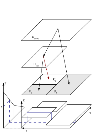
Figure 1: A sketch of the algorithm for an evolution variable $q$, one additional variable $z$, and no further parameters $\xi$. The top of the figure shows how the leaf cells (in the third plane from the top, shown here after two cell splits) are organized in a binary tree structure starting from the root cell $U_{((12)3)}$. The bottom of the figure sketches the overestimate $R$. To the left of the overestimate, the Sudakov exponent corresponding to $R$, $F(q)=-\ln\Delta_{R}(q|1)$ is shown. Here we assume that the absolute upper bound on the evolution variable is $q<1$, thus the first step to draw an event starting from a scale $Q$ is to solve $s(Q)=-\ln{\bf rnd}+F(Q)=F(q)$ for q (indicated by the dashed blue line). A $z$ value is then sampled in the cells containing the $q$ value just chosen: The cell integrals over $z$ are computed to only reflect the subtree consisting of the black arrows, and the tree structure is traversed only along the corresponding paths, selecting either of the children cells with weight given by the respective integral. Within the boundaries of a leaf cell selected by this procedure, a $z$ value is drawn flat. This corresponds to drawing a $z$ value from the distribution sketched by the solid blue line, the overestimate $R$ at fixed $q$.

The root cell of the tree spans the whole sampling volume and is the only cell present at the initial stage of the algorithm. Children cells are produced in an adaption step, iteratively building up the cell tree through splitting a cell into two children cells. This procedure aims at improving the algorithm’s efficiency along with gaining more detailed information on the target splitting kernel, i.e. a more fine-grained overestimate closer to it.

In order to achieve this, each cell always monitors its efficiency, which is defined as the ratio of the number of accepted points divided by the number of proposed points and thus gives a measure of the overall performance of the Sudakov veto algorithm. If this efficiency drops below a user-supplied threshold, the cell is considered ‘bad’. With a frequency decreasing as the efficiency of the algorithm increases, and on encounter of a bad cell, a potential splitting of the cell is determined to further increase the efficiency of the algorithm.

To obtain an optimal hyper-plane along which the cell should be split, each cell histograms projections of the average target kernel value onto each variable dimension $k$, $\langle P\rangle_{k}(x_{k})$. The dimension $k$ (which here may refer to either the evolution variable, one of the additional degrees of freedom or any of the external parameters) orthogonal to this hyperplane, and the split point $x_{k}$ (out of a number of possible split points well inside the cell’s boundaries) defined by the intersection of the hyperplane and this direction are determined to maximize a ‘gain’ measure, defined as

$$\text{gain}_{k}(x_{k})=\frac{\left|\int_{x_{k}^{-}}^{x_{k}}\langle P\rangle_{k}(x){\rm d}x-\int_{x_{k}}^{x_{k}^{+}}\langle P\rangle_{k}(x){\rm d}x\right|}{\int_{x_{k}^{-}}^{x_{k}^{+}}\langle P\rangle_{k}(x){\rm d}x}\ .$$ (4)

Here, $x_{k}^{\pm}$ denote the cell’s boundaries in the variable $x_{k}$. For reasons of performance and simplicity, the current implementation uses a two-bin histogram per dimension, and $x_{k}=(x_{k}^{-}+x_{k}^{+})/2$, leaving only the choice of dimension to maximize the gain measure: If the behaviour of $P$ is rather flat when projected on one dimension $k$, this dimension will receive a small gain measure, and projections showing more variance in $P$ are more likely to be split along. Again, a user-supplied parameter can steer the behaviour of the adaption by considering only those splits to be worth performed, if the gain exceeds some value.

Out of the two children cells the target density is being presampled in that cell which did not contain the maximum point used before to get a new estimate of the maximum. The number of presampling points per cell is another user-defined parameter. The choice of this parameter has to be carried out in view of the compensation procedure to be defined in the next section with a trade-off between the time needed for presampling and the time lost by the number of events to be vetoed by the compensation procedure. There is no general rule on how it is to be determined. Experience gained so far shows that few thousand presampling points are an acceptable compromise.

3 Compensating for New Maxima

Since the true maximum of the target kernel can never be determined with probability one from the presampling procedure, care has to be taken on what constraints need to be imposed on the sampling procedure once a point has been encountered exceeding the currently used maximum. For a sufficiently large number of presampling points one may reside on the statement that these points are rare and generated distributions will not show any effect on the erroneous overestimate. Thinking about the overall efficiency of the algorithm in performing its function of acting as a continuous source of unweighted events with the smallest possible overhead, this is certainly not a criterion to base an implementation on.

To define the method of compensation, we first introduce the notion of missing events in a given cell. As for the cell’s integral, each parent cell carries the sum of the missing events of its children cells. The number of missing events is not limited to be positive. In case it is positive, the corresponding cell needs to be oversampled, i.e. the algorithm is forced to sample events in cells with a positive number of missing events, lowering this number in the selected cell if it is larger than zero. Oversampling is imposed on the algorithm as long as there are cells with a positive count of missing events. Conversely, if the missing event count is negative, a cell needs to be undersampled. If such a cell is selected, its missing event count is increased, if it is smaller than zero and the selection is vetoed, triggering a new cell selection. The behaviour of the algorithm in a compensating state is illustrated in figure 2.

Figure 2: A sketch of the algorithm in a setup similar to figure 1, now sketching the situation upon encounter of a new overestimate. The new overestimate gave rise to different numbers of events expected in each cell (solid rectangles in the lower part), as compared to the number of events expected with the old overestimate (dotted rectangles). The difference between these determines the number of missing events per cell (see text for more details). In the sketch given here, the cells $U_{2}$ and $U_{3}$ would receive a positive number of missing events (forcing sampling in these cells as indicated by the black arrows), whereas cell $U_{1}$ would contain a negative count of missing events, triggering vetoes of attempts to sample points in this cell (indicated by the red arrow).

Upon encounter of a new maximum $w_{c}^{\prime}>w_{c}$, the number of missing events associated to this change is calculated for each cell as

$$N^{\text{miss}}_{c}=N_{c}\left(\frac{p^{\prime}_{c}}{p_{c}}-1\right)\ .$$ (5)

Here, $N_{c}$ is the number of proposal events already generated in the cell, and $p_{c}$ ($p^{\prime}_{c}$) denotes the probability to select cell $c$ using the old (new) overestimate value for events above the infrared cutoff. $p_{c}$ is calculated from the knowledge of projections of the overestimate kernel in dependence on the additional parameter point $\xi$ and the hard scale $Q$ as

$$p_{c}=\frac{\int_{c}R(q;z;\xi)\Delta_{R}(q|Q;\xi){\rm d}^{n}z\ {\rm d}q}{1-\Delta_{R}(\mu|Q;\xi)}\ .$$ (6)

$N^{\text{miss}}_{c}$ is then added to each cell’s current missing event count. Note that undersampling, $N^{\text{miss}}_{c}<0$ appears in the cells not containing the newly encountered maximum owing to the change in normalization of the overestimate density for events above the infrared cutoff. Eq. 5 ensures that within the currently accumulated statistics proposal events are always distributed according to the last encountered maximum, provided the algorithm has been stopped in a state where it is not anymore forced to perform over- or undersamplings. This is evident by rewriting eq. 5 as

$$N^{\text{miss}}_{c}=\frac{N_{c}}{\langle N\rangle_{c}}\left(\langle N^{\prime}\rangle_{c}-\langle N\rangle_{c}\right)$$ (7)

where $\langle N\rangle_{c}=Np_{c}$ ($\langle N^{\prime}\rangle_{c}=Np^{\prime}_{c}$) is the number of expected events in cell $c$ for the total number of generated events, $N$. The difference in brackets is the number of missing events in the absence of fluctuations due to a finite number of generated events, and the factor in front of it takes into account the currently accumulated statistics, i.e. how much the population of the cell differs from its expected population.

4 The Cell Selection Algorithm

In this section the complete algorithm to generate events as implemented in ExSample is defined. We here skip those parts connected to monitoring the efficiency of and splitting a cell. Proposal events according to ${\rm d}S_{R}(q|Q;z;\xi)$ as required by the Sudakov veto algorithm are generated by first deciding, if there has been an event at the infrared cutoff or otherwise selecting a proposal cell according to algorithm 1.

  calculate sub tree hash $h(Q;\xi)$ and collect projections

  loop

     solve rnd$=\Delta_{R}(q|Q;\xi)\theta(q-\mu)$ for $q$

     if $q=\mu$ then

        return  event at infrared cutoff

     end if

     collect cell integrals and missing event counters

     cell $\leftarrow$ root cell

     while cell is not a leaf do

        if $N^{\text{miss}}_{\text{firstChild(cell)}}>0\wedge N^{\text{miss}}_{\text{secondChild(cell)}}\leq 0$ then

           cell $\leftarrow$ firstChild(cell)

        else if $N^{\text{miss}}_{\text{firstChild(cell)}}\leq 0\wedge N^{\text{miss}}_{\text{secondChild(cell)}}>0$ then

           cell $\leftarrow$ secondChild(cell)

        else

           if $\mathbf{rnd}<I_{\text{firstChild(cell)}}/I_{\text{cell}}$ then

              cell $\leftarrow$ firstChild(cell)

           else

              cell $\leftarrow$ secondChild(cell)

           end if

        end if

     end while

     if $N^{\text{miss}}_{\text{cell}}=0$ then

        return  cell

     else if $N^{\text{miss}}_{\text{cell}}>0$ then

        $N^{\text{miss}}_{\text{cell}}\leftarrow N^{\text{miss}}_{\text{cell}}-1$

        return  cell

     else if $N^{\text{miss}}_{\text{cell}}<0$ then

        $N^{\text{miss}}_{\text{cell}}\leftarrow N^{\text{miss}}_{\text{cell}}+1$

     end if

  end loop

Algorithm 1 The cell selection algorithm.

Once a proposal cell has been selected, a proposal event is drawn by sampling the remaining degrees of freedom $z$ in the selected cell with uniform distribution. Except for the compensating cell selection algorithm outlined above, the Sudakov veto algorithm proceeds without modification.

5 Examples and Validation

ExSample has been validated for various ‘toy’ splitting kernels and within the realistic application of a parton shower and POWHEG matching implementation. In this section we present simple examples of distributions obtained by using ExSample, mainly to illustrate the basic functionality.

Figure 3 shows the results obtained by the adaptive Sudakov veto algorithm, using a kernel density showing the generic behaviour of a QCD splitting function with running $\alpha_{s}$. Perfect agreement with a numerical integration is found. In addition, figure 4 shows the functionality of the compensation procedure by comparing results for the same distribution but different numbers of presampling points used in the algorithm, which are all consistent with each other.

Figure 3: A Sudakov-type distribution with a QCD splitting function type kernel density as sampled by ExSample using the adaptive Sudakov veto algorithm. The vertical axis corresponds to the evolution variable $q$, the horizontal to a variable similar to a momentum fraction. Shown are few sampled events, projections of the generated distribution versus the result from a numerical integration, and the the cell grid produced.

Figure 4: The same distribution as shown in the upper left panel of figure 3, now sampled with a different number of presampling points proving functionality of the compensation procedure.

In figure 5 the results of sampling a Sudakov-type distribution in the presence of additional parameters are shown. In this example, a quark splitting function multiplied by a power law in $x/z$ has been used, where $x$ is the additional parameter and $z$ is the momentum fraction variable to be sampled. The sampled distributions in various bins of the additional parameter $x$ have been compared to a numerical integration. Full agreement has been found here. The presence of adaption splits in the parameter dimension has explicitly been checked for this example.

Figure 5: Distributions for a Sudakov-type distribution using a quark splitting function, multiplied by a power law in $x/z$. Shown are the sampled distribution for the evolution variable $q$ and momentum fraction $z$ in various bins of the additional parameter $x$. The distributions are compared to a numerical integration, proving full functionality of the sampling in presence of additional parameters.

We also use this example, which closely resembles initial state backward evolution of a parton shower at small values of the momentum fraction $x$, to asses the improvements obtained by the adaptive sampling algorithm. Particularly, we count the number of vetoed points encountered when requiring the same number of events while limiting the allowed number of cell splits. This way, a direct comparison of very coarse to increasingly finer overestimates is performed. The results are presented in figure 6, showing an exponential improvement with the number of splits performed.

Figure 6: Performance of the algorithm measured as a ratio of the number of vetoed points to the number of events requested as a function of the number of cell splits allowed. An exponential improvement is seen as more and more splits are considered. In this example, requesting $500000$ events, a maximum of $27$ splits occured. The very efficient region from $18$ splits onward with below three vetoes per generated event has been reached after about $40000$ generated events.

6 Conclusions

The sampling of Sudakov-type distributions is at the heart of all current parton shower and POWHEG NLO matching implementations. In this paper we have introduced the C++ library ExSample, which targets at adaptive sampling of these distributions as defined from a splitting kernel, which – in general – may only be known through a function call.

Additional parameters, such as typically encountered dependencies on incoming parton momentum fractions or the full dependence on a phase space point governing a hard scattering process, can be dealt with in full generality. ExSample has been validated in ‘toy’ as well as realistic setups, showing full functionality of the implementation.

Appendix A Availability and Installation

ExSample is available from

http://www.desy.de/~platzer/software/
        exsample-1.0.tar.gz

It is a complete header based library, depending additionally only on the presence of boost headers boost . An installation procedure is thus not required except for making the ExSample headers available to the client code during compilation by including the header file exsample.h. ExSample is published under the GNU General Public License version 2 gpl2 and can thus be freely used and redistributed.

The distribution contains extensive documentation, several examples of usage, as well as an implementation for standard sampling and adaptive Monte Carlo integration, of which ExSample is capable as well.

References

- (1) M. Bähr et al., Eur. Phys. J. C58, 639 (2008), 0803.0883.
- (2) T. Sjöstrand, S. Mrenna, and P. Skands, Comput. Phys. Commun. 178, 852 (2008), 0710.3820.
- (3) T. Gleisberg et al., JHEP 02, 007 (2009), 0811.4622.
- (4) M. H. Seymour, Comp. Phys. Commun. 90, 95 (1995), hep-ph/9410414.
- (5) M. Bengtsson and T. Sjostrand, Phys. Lett. B185, 435 (1987).
- (6) M. Bengtsson and T. Sjostrand, Nucl. Phys. B289, 810 (1987).
- (7) E. Norrbin and T. Sjöstrand, Nucl. Phys. B603, 297 (2001), hep-ph/0010012.
- (8) G. Miu and T. Sjostrand, Phys. Lett. B449, 313 (1999), hep-ph/9812455.
- (9) P. Nason, JHEP 11, 040 (2004), hep-ph/0409146.
- (10) G. Corcella et al., (2002), hep-ph/0210213.
- (11) T. Sjöstrand, S. Mrenna, and P. Skands, JHEP 05, 026 (2006), hep-ph/0603175.
- (12) A. Buckley et al., Phys. Rept. 504, 145 (2011), 1101.2599.
- (13) S. Platzer and M. Sjodahl, Eur.Phys.J.Plus 127, 26 (2012), 1108.6180.
- (14) L. Lönnblad, ACDC – The Auto Compensating Divide-and-Conquer Phase Space Generator.
- (15) S. Jadach, Comput. Phys. Commun. 152, 55 (2003), physics/0203033.
- (16) http://www.boost.org.
- (17) http://www.gnu.org/licenses/.