Density functional for ternary non-additive hard sphere mixtures

Abstract

Based on fundamental measure theory, a Helmholtz free energy density functional for three-component mixtures of hard spheres with general, non-additive interaction distances is constructed. The functional constitutes a generalization of the previously given theory for binary non-additive mixtures. The diagrammatic structure of the spatial integrals in both functionals is of star-like (or tree-like) topology. The ternary diagrams possess a higher degree of complexity than the binary diagrams. Results for partial pair correlation functions, obtained via the Ornstein-Zernike route from the second functional derivatives of the excess free energy functional, agree well with Monte Carlo simulation data.

I Introduction

Rosenfeld’s fundamental measures theory (FMT) for additive hard sphere mixtures rosenfeld89 ; kierlik90 has become a cornerstone of classical density functional theory (DFT) evans79 . FMT features in numerous applications to a wide variety of interesting phenomena in liquids roth10review ; tarazona08review ; lutsko10review . In additive hard sphere mixtures the interaction distance between unlike components is taken to be the arithmetic mean of the (like-species) diameters. Additive mixtures are often considered as prototypical in the description of liquid mixtures. Nevertheless, non-additivity is a generic feature kahl90 that arises very naturally in effective interactions, e.g. due to the depletion effect louis01depl , or when integrating out solvent degrees of freedom in electrolytes kalcher10 ; kalcher10jcp . A generalization of FMT to binary non-additive hard sphere (NAHS) mixtures schmidt04nahs was based on the scalar version of the additive hard sphere functional kierlik90 , and has been used successfully in the investigation of bulk hopkins10nahs ; ayadim10 ; hopkins11natpl and of interfacial hopkins11nawe phenomena that occur in NAHS mixtures.

Recently significant progress has been made in the formalization of the mathematical structure of FMT. This includes i) insights into the geometry of the non-local aspects of the theory, i.e. the algebraic group structure and symmetry properties of the convolution kernel matrix ${\sf K}(R,r)$ schmidt04nahs ; schmidt07nage ; schmidt11nagl , which controls the range of non-locality in the functional. Here $R$ is a fixed lengthscale and $r$ is the radial distance in three-dimensional space. Formally, ${\sf K}(R,r)$ is a $4\times 4$-matrix that is indexed by powers of lengthscale. Its remarkable algebraic properties schmidt07nage allow to view it as an object that is suitable to add or remove a layer of thickness $R$ from a given sphere. Furthermore, ii) the FMT for additive hard sphere mixtures was obtained from a tensorial-diagrammatic series in density leithall11hys . The diagrams possess star-like topology, which is an approximation of the combinatorial complexity of the exact virial expansion. Apart from a central space integral, all field points are integrations over the density field(s), as they are in the exact virial expansion. The bonds, however, are weight functions rather than Mayer functions, and possess only half the range of the (hard sphere) Mayer function. In one dimension, the result from the series is equal to Percus’ exact functional percus76 . In three dimensions it gives the Kierlik-Rosinberg form kierlik90 of FMT. The five-dimensional hard hypersphere version is investigated in detail in Ref. leithall11hys . Comparison to data from the literature for bulk structure and thermodynamics demonstrates the capability of this theory for study bulk and inhomogeneous hypersphere mixtures.

In the present work we generalize the tensorial-diagrammatic series to non-additive hard sphere interactions. We use the kernel matrix ${\sf K}(R,r)$ as a further type of bond. This enables us to represent the binary NAHS functional of Ref. schmidt04nahs as a series of diagrams that are formed by two stars, one for each species. Here the center of one star is connected to the center of the second star by a ${\sf K}$-bond. Formulating an FMT for general ternary non-additive hard sphere mixtures requires to modify this topology. Treating special cases of ternary mixtures that have a suitably high degree of additivity amounts to straightforward generalizations of Ref. schmidt04nahs . This is the case when the cross interaction between (say) species 1 and 2 is additive, and the non-additivities between 13 and 23 are coupled in a certain way (see the discussion below (1)), and hence cannot be chosen independently from each other. The general case, however requires the introduction of diagrams with different topology. Here three stars, one for each species, are connected to a central three-arm star. As laid out in detail below, all (four) inner junctions are bare space integrals, without multiplication by a one-body density. Only the outer ends carry multiplication by a (bare) density variable. We show that the theory predicts the bulk structure of ternary mixtures, via the Ornstein-Zernike route, with good quality as compared to Monte Carlo simulation data.

II Non-additive hard sphere interactions

Non-additive hard sphere mixtures possess pair potentials $v_{ij}(r)$ between species $i$ and $j$ as a function of the center-center distance $r$ of the two particles, that are given as $v_{ij}(r)=\infty$ if $r<\sigma_{ij}$, and zero otherwise. In the general case all $\sigma_{ij}$ are independent of each other, except for the trivial symmetry $\sigma_{ij}=\sigma_{ji}$. Non-additivity parameters are conventionally defined as $\Delta_{ij}=2\sigma_{ij}/(\sigma_{ii}+\sigma_{jj})-1$ for $i\neq j$, where $\Delta_{ij}\geq-1$. For additive mixtures all $\Delta_{ij}=0$. For positive non-additivity, $\Delta_{ij}>0$, the unlike components interact at a larger distance than the arithmetic mean of their diameters. For negative non-additivity, $\Delta_{ij}<0$, the interaction distance is smaller than the mean of the diameters. While a binary NAHS mixture is characterized by either positive or negative non-additivity, in ternary systems mixed cases are possible, where not all of the $\Delta_{ij}$ have the same sign. In ternary NAHS mixtures the equation of state santos05 was considered and phase stability was investigated using integral equation theory gazzillo96 . Phase equilibrium was also considered in polydisperse non-additive hard sphere systems dickinson79 ; paricaud08 .

III Density functional theory

III.1 Overview and choice of lengthscales

In order to construct an FMT for ternary NAHS mixtures, we first identify suitable lengthscales. Consistent with Rosenfeld’s additive case rosenfeld89 , we use the particle radii $R_{i}=\sigma_{ii}/2$ of each species $i=1,2,3$. For the binary mixture schmidt04nahs , the cross diameter between species 1 and 2 was decomposed as $\sigma_{12}=R_{1}+R_{12}+R_{2}$, where the lengthscale $R_{12}=\sigma_{12}-(\sigma_{11}+\sigma_{22})/2$ accounts for the non-additivity. For the ternary system, we generalize this to a decomposition of the cross diameters into sums of four contributions,

$$\sigma_{ij} =R_{i}+d_{i}+d_{j}+R_{j},$$ (1)

where $ij=12,13,23$, and the three lengthscales $d_{i}$, $i=1,2,3$, control the degrees of non-additivity. Inverting Eq. (1) is possible for ternary mixtures and yields $d_{j}=(\sigma_{ij}+\sigma_{jk}-\sigma_{ik}-\sigma_{jj})/2$; here $ijk=123$ or any permutation thereof. As a simple check, a counting exercise assures us that the number of parameters $R_{i}$ (three) and $d_{i}$ (also three) is enough to represent the six independent components of $\sigma_{ij}$. The binary case above is recovered if we set $R_{12}=d_{1}+d_{2}$. Here the relative splitting of $R_{12}$ into $d_{1}$ and $d_{2}$ is arbitrary. If we keep three species, and set $d_{1}=d_{2}=0$, then only $d_{3}\neq 0$ remains in order to control the non-additivities between 13 and between 23. For mixtures with such restricted degree of non-additivity, as mentioned above, the binary NAHS functional can be generalized easily. Figure 1 illustrates the different types of decomposition of the $\sigma_{ij}$ in binary additive (a), binary non-additive (b, c), and ternary non-additive (d) mixtures. Note that the $d_{i}$ can be negative, but that $R_{i}+d_{i}+d_{j}+R_{j}\geq 0$ must hold due to (1). Furthermore certainly $R_{i}\geq 0$.

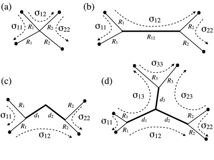
Figure 1: Illustration of the decomposition (1) of the hard sphere interaction distances $\sigma_{ij}$ into like-species particle radii $R_{i}$ and non-additivity distances $d_{i}$. Thin solid lines represent distances between a space point (dots) and a junction; thick solid lines represent the distance between two junctions. The dashed arrows indicate paths that possess length $\sigma_{ij}$ (as indicated); the sense of direction is only a guide to the eye. Decompositions are shown for the binary additive mixture (a), the binary non-additive mixture with the cross diameter being divided into three (b) and four (c) contributions, and the ternary non-additive mixture (d). The two binary cases (b) and (c) are equivalent when $R_{12}=d_{1}+d_{2}$.

As a means to control the different lengthscales in the density functional, we use the kernel matrix ${\sf K}(R,r)$ of Refs. schmidt04nahs ; schmidt07nage ; schmidt11nagl . Two of its properties render this a suitable object for the construction of the density functional: i) the four scalar Kierlik-Rosinberg weight functions (where $R$ is identified with the particle radius) feature as components and ii) matrices can be chained, ${\sf K}(R+R^{\prime},r)={\sf K}(R,r)\ast{\sf K}(R^{\prime},r)$, where the asterisk denotes the three-dimensional spatial convolution and matrix multiplication is implied on the right hand side. The three-dimensional Fourier transform of ${\sf K}(R,r)$ can be expressed as $\tilde{\sf K}(R,q)=\exp(R{\sf G})$, where $q$ is the radial distance in reciprocal space, and the (generator) matrix ${\sf G}$ depends on $q$ and is defined by its components $G_{1}^{\;\;0}=1,G_{2}^{\;\;1}=8\pi,G_{3}^{\;\;2}=1,G_{1}^{\;\;2}=-q^{2}/(4\pi),G_{0}^{\;\;3}=-q^{4}/(8\pi)$; all other $G_{\mu}^{\;\;\nu}=0$. Here the lower index indicates the row and the upper index indicates the column; all Greek indices run from 0 to 3 here and in the following. Due to the symmetry $K_{\mu}^{\;\;\nu}(R,r)=K_{3-\mu}^{\;\;3-\nu}(R,r)$ schmidt11nagl , the matrix ${\sf K}(R,r)$ has ten independent components hopkins10nahs ; schmidt11nagl . The four scalar Kierlik-Rosinberg kierlik90 weight functions $w_{\nu}(R,r)$ are contained herein, i.e. $K_{0}^{\;\;\nu}(R,r)=w_{\nu}(R,r)$, explicitly given in real space as $w_{3}(R,r)=\Theta(R-r)$, $w_{2}(R,r)=\delta(R-r)$, $w_{1}(R,r)=\delta^{\prime}(R-r)/(8\pi)$, and $w_{0}(R,r)=-\delta^{\prime\prime}(R-r)/(8\pi)+\delta^{\prime}(R-r)/(2\pi r)$. An explicit real-space expression for all further components of ${\sf K}(R,r)$ can be found in schmidt07nage .

The Mayer $f$-bond for hard spheres equals $-1$ if the two spheres overlap and vanishes otherwise. For like species the deconvolution into scalar weight functions kierlik90 can be written as $f_{ii}(r)=-\sum_{\mu=0}^{3}w_{\mu}(R,r)\ast w_{3-\mu}(R,r)\equiv-\sum_{\mu,\nu=0}^{3}w_{\mu}(R,r)M^{\mu\nu}w_{\nu}(R,r)$. Here the spatial convolution of two functions is defined as $(f\ast g)({\bf x})=\int d{\bf r}f({\bf r})g({\bf x}-{\bf r})$, and the metric ${\sf M}$ schmidt11nagl has components $M_{\mu\nu}=M^{\mu\nu}=1$ if $\mu+\nu=3$ and is zero otherwise. The crucial property of ${\sf K}(R,r)$ that we will exploit in the following is the group structure for the combined operation of matrix multiplication and (real-space) convolution. For the interactions between particles of the same species ${\sf K}(2R_{i},r)={\sf K}(R_{i},r)\ast{\sf K}(R_{i},r)$, where the convolution product implies also matrix multiplication, and the Mayer bond is just the special case $f_{ii}(r)=-w_{3}(2R_{i},r)=-K_{0}^{\;\;3}(2R_{i},r)$. We exploit the fact that several matrices can be chained schmidt07nage , in order to model the interactions between unlike species via ${\sf K}(\sigma_{ij},r)={\sf K}(R_{i},r)\ast{\sf K}(d_{i},r)\ast{\sf K}(d_{j},r)\ast{\sf K}(R_{j},r)$, where the lengthscales on the right hand side satisfy (1). Furthermore the terms on the right hand side commute (i.e. the group is Abelian schmidt07nage ). The Mayer bond between unlike species $i$ and $j$ is $f_{ij}(r)=-K_{0}^{\;\;3}(\sigma_{ij},r)$ and can hence be written as $f_{ij}(r)=-\sum_{\mu,\mu^{\prime},\nu,\tau}^{3}M^{\mu\mu^{\prime}}w_{\mu^{\prime}}(R_{i},r)\ast K_{\mu}^{\;\;\nu}(d_{i},r)\ast K_{\nu}^{\;\;\tau}(d_{j},r)\ast w_{\tau}(R_{j},r)$. This identity, as well as that for the intra-species case above, can be verified by explicit algebra, most conveniently in Fourier space, where the convolutions become mere products and algebraic theorems for trigonometric functions can be used to simplify the expressions.

III.2 Algebraic-diagrammatic structure of the free energy functional

Using the four weight functions $w_{\mu}(R_{i},r)$, we build species-dependent weighted densities $n_{\mu}(i,{\bf r})$ in the standard way via convolution with the bare density distribution of the corresponding species,

$$n_{\mu}(i,{\bf r})=w_{\mu}(R_{i},r)\ast\rho_{i}({\bf r}).$$ (2)

We use the third-rank “junction” tensor ${\sf J}$ of Ref. leithall11hys in order to couple the $n_{\mu}(i,{\bf r})$ and hence generate terms that are non-linear in densities. Let us denote the components of ${\sf J}$ by $J^{\mu\nu\tau}$. The tensor is symmetric under exchange of indices, and is non-zero only if $\mu+\nu+\tau=6$. One can specify ${\sf J}$ completely via the elements $J^{123}=J^{033}=1$, and $J^{222}=1/(4\pi)$. As a basic building block for the construction of the density functional, we use the matrix ${\sf N}(i,{\bf r})$ of weighted densities leithall11hys that is obtained by contracting the vector of weighted densities $n_{\tau}(i,{\bf r})$ with the ${\sf J}$-tensor and lowering one of the indices via contraction with the metric ${\sf M}$. Hence the components of the matrix ${\sf N}(i,{\bf r})$ are obtained as $N_{\mu}^{\;\;\nu}(i,{\bf r})=\sum_{\mu^{\prime},\tau=0}^{3}M_{\mu\mu^{\prime}}J^{\mu^{\prime}\nu\tau}n_{\tau}(i,{\bf r})$, and given explicitly by

$${\sf N}(i,{\bf r}) =\left(\begin{matrix}n_{3}(i,{\bf r})&n_{2}(i,{\bf r})&n_{1}(i,{\bf r})&n_{0}(i,{\bf r})\\ 0&n_{3}(i,{\bf r})&\frac{n_{2}(i,{\bf r})}{4\pi}&n_{1}(i,{\bf r})\\ 0&0&n_{3}(i,{\bf r})&n_{2}(i,{\bf r})\\ 0&0&0&n_{3}(i,{\bf r})\end{matrix}\right).$$ (3)

As an illustration of the power of this formalized framework, we can obtain leithall11hys the additive FMT functional as the 03-component of $\int d{\bf x}\phi_{\rm 0d}(\sum_{i}{\sf N}(i,{\bf x}))$, where the integration variable was renamed from ${\bf r}$ to ${\bf x}$, and the zero-dimensional excess free energy is

$$\phi_{\rm 0d}(\eta)\equiv(1-\eta)\ln(1-\eta)+\eta=\sum_{m=2}^{\infty}\frac{\eta^{m}}{m(m-1)},$$ (4)

with the (dummy) variable $\eta$ being the average occupation number of the zero-dimensional system. Here a function of a matrix is defined via its power series. In order to represent the mathematical structure of the integrals in the density functional, we use the diagrammatic formulation of Ref. leithall11hys , see Fig. 2 for an overview. In particular, the star topology shown in Fig. 2a constitutes the relevant type of diagram for additive hard sphere mixtures. The center of the diagram represents the integration variable ${\bf x}$, the arms represent the weight functions $w_{\mu}(r)$, and the filled symbols represent the one-body density $\rho_{i}({\bf r})$ at space point(s) ${\bf r}$. All spatial variables are integrated over. The number of arms equals the order in density. Summing up all orders and using the coefficients of the power series of $\phi_{\rm 0d}$ yields the Kierlik-Rosinberg free energy functional leithall11hys .

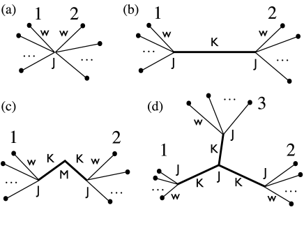
Figure 2: Illustration of the topology of the diagrams that constitute the density series of the FMT free energy functional for various hard sphere mixtures. The one-body density distribution of each species $\rho_{i}({\bf r})$ (represented by a filled symbol) is connected by weight function bonds, ${\sf w}=(w_{0},w_{1},w_{2},w_{3})$ (thin lines), to a central space integral (junction). The different topologies are for the binary additive hard spheres (a), binary non-additive hard spheres (b,c) and ternary non-additive hard sphere mixtures (d). The numbers indicate the different species. In (b,c,d) the the junctions are joined by convolution kernel bonds ${\sf K}$. The bonds that meet at a junction are multiplied by third-rank tensors ${\sf J}$. Multiplying with the metric ${\sf M}$ at the center of (c) joins the two ${\sf K}$-bonds and restores the topology of (d). All junctions and all end points are integrated over.

In the following we require only the last column of the $l$-th power of the density matrix, obtained formally as

$$\psi^{(l)}_{\nu}(i,{\bf r}) ={\sf N}^{l}(i,{\bf r})\cdot(0,0,0,1)^{\rm t},$$ (5)

where ${\sf N}^{l}(i,{\bf r})$ indicates the $l$-th (matrix) power of ${\sf N}(i,{\bf r})$, the dot represents the multiplication between a matrix and a vector and the superscript t indicates transposition. Explicitly, the four components in (5) are

$$\psi_{0}^{(l)}(i,{\bf r}) =ln_{0}n_{3}^{l-1}-l(l-1)n_{1}n_{2}n_{3}^{l-2}$$

$$\quad\quad+\frac{l(l-1)(l-2)}{24\pi}n_{2}^{3}n_{3}^{l-3}$$ (6)

$$\psi_{1}^{(l)}(i,{\bf r}) =ln_{1}n_{3}^{l-1}-\frac{l(l-1)}{8\pi}n_{2}^{2}n_{3}^{l-2}$$ (7)

$$\psi_{2}^{(l)}(i,{\bf r}) =ln_{2}n_{3}^{l-1}$$ (8)

$$\psi_{3}^{(l)}(i,{\bf r}) =n_{3}^{l},$$ (9)

where the superscripts of the weighted densities indicate (scalar) powers, the weighted densities are those of species $i$, i.e. $n_{\mu}\equiv n_{\mu}(i,{\bf r})$, and the arguments have been omitted for clarity.

For non-additive mixtures we “transport” the expressions (6)-(9) via convolution with ${\sf K}(d_{i},r)$. We hence obtain a fourvector for each species $i$, indexed by $\mu=0,1,2,3$, and given as

$$\Phi_{\mu}^{(l)}(i,{\bf r}) =\sum_{\nu=0}^{3}{\sf K}_{\mu}^{\;\;\nu}(d_{i},r)\ast\psi_{\nu}^{(l)}(i,{\bf r}).$$ (10)

These objects serve as ansatz functions for representing the free energy density; they are specific for each species (indicated by the argument $i$), are of $l$-th order in density, and carry the dimension of (length)^3-μ.

III.3 Rewriting the binary non-additive hard sphere functional

Using the above definitions, we can write the density functional for binary non-additive hard sphere mixtures schmidt04nahs as

$$F_{\rm exc}[\rho_{1},\rho_{2}] =k_{B}T\int d{\bf y}\sum_{\mu,\nu=0}^{3}M^{\mu\nu}\sum_{k,l=0}^{\infty}\frac{(k+l-2)!}{k!\,l!}$$

$$\qquad\qquad\times\Phi_{\mu}^{(k)}(1,{\bf y})\Phi_{\nu}^{(l)}(2,{\bf y}),$$ (11)

where we take the convention that the factorial vanishes for negative arguments and we have renamed the spatial integration variable from ${\bf r}$ to ${\bf y}$. The scalar coefficients inside of the double sum over $k,l$ are those in the Taylor expansion of the zero-dimensional excess free energy, which for a binary mixture is $\phi_{\rm 0d}(\eta_{1}+\eta_{2})=\sum_{k,l=1}^{\infty}\binom{k+l}{k}\eta_{1}^{k}\eta_{2}^{l}/[(k+l)(k+l-1)]$. Writing the coefficients as $\binom{k+l}{k}/[(k+l)(k+l-1)]=(k+l-2)!/(k!\,l!)$ gives the form in (11).

A closed expression for the series (11) can be obtained. This is identical to the previously given schmidt04nahs form of the binary functional

$$F_{\rm exc}[\rho_{1},\rho_{2}]=k_{B}T$$

$$\times\int d{\bf x}\int d{\bf x}^{\prime} \sum_{\mu,\nu=0}^{3}K^{\mu\nu}(d_{1}+d_{2},{\bf x}-{\bf x}^{\prime})\Phi_{\mu\nu}({\bf x},{\bf x}^{\prime}),$$ (12)

where the components of the free energy tensor are

$$\Phi_{\mu\nu}({\bf x},{\bf x}^{\prime}) =\sum_{\alpha,\beta=0}^{3}A_{\mu\alpha}(1,{\bf x})A_{\nu\beta}(2,{\bf x}^{\prime})$$

$$\qquad\times\phi_{\rm 0d}^{[\alpha+\beta]}\big{(}n_{3}(1,{\bf x})+n_{3}(2,{\bf x}^{\prime})\big{)},$$ (13)

where $\phi_{\rm 0d}^{[\alpha]}(\eta)\equiv d^{\alpha}\phi_{\rm 0d}(\eta)/d\eta^{\alpha}$ is the $\alpha$-th derivative of the $0d$ excess free energy. Explicit expressions for the coefficients in (13) are

$$A_{01}(i,{\bf x}) =n_{0}(i,{\bf x}),$$

$$A_{02}(i,{\bf x}) =n_{1}(i,{\bf x})n_{2}(i,{\bf x}),$$

$$A_{03}(i,{\bf x}) =\frac{[n_{2}(i,{\bf x})]^{3}}{24\pi},$$

$$A_{11}(i,{\bf x}) =n_{1}(i,{\bf x}),$$ (14)

$$A_{12}(i,{\bf x}) =\frac{[n_{2}(i,{\bf x})]^{2}}{8\pi},$$

$$A_{21}(i,{\bf x}) =n_{2}(i,{\bf x}),$$

$$A_{30}(i,{\bf x}) =1,$$

where $i$ labels the species [$i=1,2$ for (13)]. In the above we have exploited the convolution property

$$K^{\mu\nu}(d_{1}+d_{2},{\bf x}-{\bf x}^{\prime})=$$

$$\sum_{\tau,\tau^{\prime}=0}^{3}M_{\tau\tau^{\prime}}\int d{\bf y} K^{\mu\tau}(d_{1},{\bf x}-{\bf y})K^{\tau^{\prime}\nu}(d_{2},{\bf x}^{\prime}-{\bf y}).$$ (15)

Due to the group structure of the convolution kernels schmidt07nage ; schmidt11nagl , the identity $K_{\mu}^{\;\;\nu}(d_{i}+d_{j},r)=\sum_{\tau=0}^{3}K_{\mu}^{\;\;\tau}(d_{i},r)\ast K_{\tau}^{\;\;\nu}(d_{j},r)$ holds, such that the lengthscale $R_{12}\equiv\sigma_{12}-(\sigma_{11}+\sigma_{22})/2$ of the binary functional schmidt04nahs is recovered as $R_{12}=d_{1}+d_{2}$. The structure of the diagrams corresponding to (12) is shown in Fig. 2b and that corresponding to (11) is shown in Fig. 2c.

III.4 Constructing a ternary non-additive hard sphere functional

The benefit of re-writing the binary functional in the form (11) is that this allows for straightforward generalization to three-component mixtures as

$$F_{\rm exc}[\rho_{1},\rho_{2},\rho_{3}]=k_{B}T\int d{\bf x}\sum_{\mu,\nu,\tau=0}^{3}J^{\mu\nu\tau}$$

$$\times\sum_{k,l,m=0}^{\infty}\frac{(k+l+m-2)!}{k!\,l!\,m!}\Phi_{\mu}^{(k)}(1,{\bf x})\Phi_{\nu}^{(l)}(2,{\bf x})\Phi_{\tau}^{(m)}(3,{\bf x}),$$ (16)

where $(k+l+m-2)!/(k!\,l!\,m!)$ is the coefficient of order $\eta_{1}^{k}\eta_{2}^{l}\eta_{3}^{m}$ in the Taylor expansion of $\phi_{\rm 0d}(\eta_{1}+\eta_{2}+\eta_{3})$. Again a closed expression can be obtained, which is in the form

$$F_{\rm exc}[\rho_{1},\rho_{2},\rho_{3}]= k_{B}T\int d{\bf y}\int d{\bf x}\int d{\bf x}^{\prime}\int d{\bf x}^{\prime\prime}\sum_{\mu,\nu,\tau=0}^{3}J^{\mu\nu\tau}\sum_{\mu^{\prime},\nu^{\prime},\tau^{\prime}=0}^{3}K_{\mu}^{\;\;\mu^{\prime}}(d_{1},{\bf x}-{\bf y})$$

$$\quad\quad\times K_{\nu}^{\;\;\nu^{\prime}}(d_{2},{\bf x}^{\prime}-{\bf y})K_{\tau}^{\;\;\tau^{\prime}}(d_{3},{\bf x}^{\prime\prime}-{\bf y})\Phi_{\mu^{\prime}\nu^{\prime}\tau^{\prime}}({\bf x},{\bf x}^{\prime},{\bf x}^{\prime\prime}),$$ (17)

where

$$\Phi_{\mu\nu\tau}({\bf x},{\bf x}^{\prime},{\bf x}^{\prime\prime})=$$

$$\sum_{\alpha,\beta,\gamma=0}^{3}A_{\mu\alpha}(1,{\bf x})A_{\nu\beta}(2,{\bf x}^{\prime})A_{\tau\gamma}(3,{\bf x}^{\prime\prime})$$

$$\quad\times\phi_{\rm 0d}^{[\alpha+\beta+\gamma]}\big{(}n_{3}(1,{\bf x})+n_{3}(2,{\bf x}^{\prime})+n_{3}(3,{\bf x}^{\prime\prime})\big{)}.$$ (18)

Eqs. (18) and (17) together with Eq. (14) (where $i=1,2,3$) prescribe the DFT for the general ternary hard sphere mixture. It is straightforward to verify that this functional reduces, in the corresponding limits, to the FMT for additive ternary hard sphere mixtures rosenfeld89 ; kierlik90 , and for binary NAHS mixtures schmidt04nahs . The diagrammatical structure of (17) is shown in Fig. 2d.

IV Results for bulk fluid structure

We test the theory by calculating the partial two-body direct correlation functions for bulk fluids from $c_{ij}(|{\bf r}-{\bf r}^{\prime}|)=-(k_{B}T)^{-1}\left.\delta^{2}F_{\rm exc}/\delta\rho_{i}({\bf r})\delta\rho_{j}({\bf r}^{\prime})\right|_{\rho_{k}=\mathrm{const}}$. Analytic expressions for the corresponding expressions $\tilde{c}_{ij}(q)$ in Fourier space can be obtained. Inserting these into the Ornstein-Zernike equation for ternary mixtures and Fourier transforming numerically yields partial pair correlation functions $g_{ij}(r)$. Such results are shown in Fig. 3 for symmetric mixtures, $\sigma_{11}=\sigma_{22}=\sigma_{33}\equiv\sigma$, with varying degree of non-additivity $\Delta_{12}=\Delta_{23}=\Delta_{23}\equiv\Delta$, and at equal (and constant) bulk densities, $\rho_{1}=\rho_{2}=\rho_{3}$. We choose the overall packing fraction as $\eta=\sum_{i}\pi\rho_{i}\sigma_{ii}^{3}/6=0.2$ and compare to benchmark Monte Carlo simulation results for 1023 particles, obtained with $10^{6}$ attempted moves per particle of which the initial $10^{5}$ moves were used for equilibration. Except for (numerically) small core violation, the OZ results reproduce the simulation data very well. This is also the case for the slightly higher total packing fraction, $\eta=0.25$, where again MC and DFT data are compared in Fig. 4.

Figure 3: Partial pair correlation function $g_{ij}(r)$ for symmetric ternary non-additive hard sphere mixtures with $\sigma_{11}=\sigma_{22}=\sigma_{33}\equiv\sigma$ for varying degree of non-additivity $\Delta_{12}=\Delta_{23}=\Delta_{13}\equiv\Delta=-0.1,0,0.1$ as a function of the scaled distance $r/\sigma$. Symbols denote Monte Carlo data; lines represent DFT results. Shown are the like correlation function $g_{11}(r)$ (solid lines and crosses) and the unlike correlation function $g_{12}(r)$ (dashed lines and pluses). The results for $\Delta=0$ (0.1) are shifted upwards by two (four) units.

Figure 4: Same as Fig. 3, but for total packing fraction $\eta=0.25$.

In order to consider a fully asymmetric case, we have chosen the $\sigma_{ij}$ in order to mimick the correlations that were obtained in Molecular Dynamics simulations of an aqeuous binary salt solution kalcher10jcp . Here the solvent is at large packing fraction and both types of ions are at vanishing concentration. In this case the model parameters can be tuned to mimick the simulation data (not shown). This constitutes a step towards possible applications of the current theory to electrolyte solutions. However, for mixtures with very asymmetric size ratios one would expect to find similar shortcomings as are present in the additive FMT herring06prl and indeed Percus-Yevick theory.

V Conclusions

In conclusion, we have presented a fundamental measure functional for ternary NAHS mixtures. The mathematical structure of the functional is based on a diagrammatic expansion in density with star-like (tree-like) topology of the diagrams. We have shown that pair correlation functions obtained from the density functional via the Ornstein-Zernike route agree well with computer simulation data. Possible applications of the current theory include its use as a reference system in modeling electrolytes in bulk and in inhomogeneous situations. Furthermore, considering one-dimensional cases, see Ref. santos08oned for the exact solution of bulk properties of binary mixtures, could be interesting.

It is worthwhile to discuss possible generalization to mixtures with more than three components. The general ternary case presented here rests crucially on the decomposition of the interaction distances $\sigma_{ij}$ into suitable length scales $R_{i}$ and $d_{i}$, cf. (1). This allowed to use suitable diagrams with tree-like structure, cf. Fig. 2d. However, (1) does not have a general solution (for $R_{i}$ and $d_{i}$ once the $\sigma_{ij}$ are prescribed) for $M\geq 4$ components. That this is true can be gleaned from the fact that the $\sigma_{ij}$ are $M(M+1)/2$ independent constants, whereas the $R_{i}$ and $d_{i}$ constitute only $2M$ free parameters. These numbers, seemingly by accident, match in the special case $M=3$. Hence we can conclude that possible extensions to four and more components requires further changes in the mathematical structure of the present FMT.

- (1) Y. Rosenfeld, Phys. Rev. Lett. 63, 980 (1989).
- (2) E. Kierlik and M. L. Rosinberg, Phys. Rev. A 42, 3382 (1990).
- (3) R. Evans, Adv. Phys. 28, 143 (1979).
- (4) R. Roth, J. Phys.: Condensed Matter 22, 063102 (2010).
- (5) P. Tarazona, J. A. Cuesta, and Y. Martinez-Raton, Lect. Notes Phys. 753, 247 (2008).
- (6) J. F. Lutsko, Adv. Chem. Phys. 144, 1 (2010).
- (7) G. Kahl, J. Chem. Phys. 93, 5105 (1990).
- (8) A. A. Louis and R. Roth, J. Phys.: Condensed Matter 13, L777 (2001).
- (9) I. Kalcher, J. C. F. Schulz, and J. Dzubiella, Phys. Rev. Lett. 104, 097802 (2010).
- (10) I. Kalcher, J. C. F. Schulz, and J. Dzubiella, J. Chem. Phys. 133, 164511 (2010).
- (11) M. Schmidt, J. Phys.: Condensed Matter 16, L351 (2004).
- (12) P. Hopkins and M. Schmidt, J. Phys.: Condensed Matter 22, 325108 (2010).
- (13) A. Ayadim and S. Amokrane, J. Phys.: Condensed Matter 22, 035103 (2010).
- (14) P. Hopkins and M. Schmidt, J. Phys.: Condensed Matter 23, 325104 (2011).
- (15) P. Hopkins and M. Schmidt, Phys. Rev. E 83, 050602(R) (2011).
- (16) M. Schmidt and M. R. Jeffrey, J. Math. Phys. 48, 123507 (2007).
- (17) M. Schmidt, Mol. Phys. 109, 1253 (2011).
- (18) G. Leithall and M. Schmidt, Phys. Rev. E 83, 021201 (2011).
- (19) J. K. Percus, J. Stat. Phys. 15, 505 (1976).
- (20) A. Santos, M. L. de Haro, and S. B. Yuste, J. Chem. Phys. 122, 024514 (2005).
- (21) D. Gazzillo, Mol. Phys. 84, 303 (1996).
- (22) E. Dickinson, Chem. Phys. Lett. 66, 500 (1979).
- (23) P. Paricaud, Phys. Rev. E 78, 021202 (2008).
- (24) A. R. Herring and J. R. Henderson, Phys. Rev. Lett. 97, 148302 (2006).
- (25) A. Santos, Phys. Rev. E 76, 062201 (2007).