Self-assembly of bi-functional patchy particles with anisotropic shape into polymers chains: theory and simulations

Abstract

Concentrated solutions of short blunt-ended DNA duplexes, down to 6 base pairs, are known to order into the nematic liquid crystal phase. This self-assembly is due to the stacking interactions between the duplex terminals that promotes their aggregation into poly-disperse chains with a significant persistence length. Experiments show that liquid crystals phases form above a critical volume fraction depending on the duplex length. We introduce and investigate via numerical simulations, a coarse-grained model of DNA double-helical duplexes. Each duplex is represented as an hard quasi-cylinder whose bases are decorated with two identical reactive sites. The stacking interaction between terminal sites is modeled via a short-range square-well potential. We compare the numerical results with predictions based on a free energy functional and find satisfactory quantitative matching of the isotropic-nematic phase boundary and of the system structure. Comparison of numerical and theoretical results with experimental findings confirm that the DNA duplexes self-assembly can be properly modeled via equilibrium polymerization of cylindrical particles and enables us to estimate the stacking energy.

I Introduction

Self-assembly is the spontaneous organization of matter into reversibly-bound aggregates. In contrast to chemical synthesis where molecular complexity is achieved through covalent bonds, in self-assembled structures the molecules or supramolecular aggregates spontaneously form following the minimization of their free energy. Self-assembly is ubiquitous in nature and can involve the structuring of elementary building blocks of various sizes, ranging from simple molecules (e.g. surfactants) to the mesoscopic units (e.g. colloidal particles), thus being of topical interest in several fields, including soft matter and biophysics Hamley (2007); Glotzer (2004); Whitesides and Boncheva (2002). Understanding and thus controlling the processes of self-assembly is important in material science and technology for devicing new materials whose physical properties are controlled by tuning the interactions of the assembled components Workum and Douglas (2006); Mirkin et al. (1996); Manoharan et al. (2003); Cho et al. (2005); Yi et al. (2004); Cho et al. (2005); Starr et al. (2003); Starr and Sciortino (2006); Stupp et al. (1993); Doye et al. (2007).

A particular but very interesting case of self-assembly occurs when the anisotropy of attractive interactions between the monomers favors the formation of linear or filamentous aggregates, i.e. linear semi-flexible, flexible or rigid chains. A longstanding example is provided by the formation of worm-like micelles of amphiphilic molecules in water or microemulsions of water and oil which are stabilized by amphiphilic molecules . If supramolecular aggregates possess a sufficient rigidity the system may exhibit liquid crystal (LC) ordering even if the self-assembling components do not have the required shape anisotropy to guarantee the formation of nematic phases. An intense experimental activity has been dedicated to the study of nematic transitions in micellar systems Khan (1996); van der Schoot and Cates (1994a); Kuntz and Walker (2008). Another prominent case is that of formation of fibers and fibrils of peptides and proteins Jung and Mezzenga (2010); Lee (2009); Ciferri (2007); Aggeli et al. (2003). Over last $50$ years LC phases have been also observed in solutions of long duplex B-form DNA composed of $10^{2}$ to $10^{6}$ base pairs Robinson (1961); Livolant et al. (1989); Merchant and Rill (1997); Tombolato and Ferrarini (2005) and in the analogous case of filamentous viruses Tombolato et al. (2006); Barry et al. (2009); Grelet and Fraden (2003); Tomar et al. (2007); Minsky et al. (2002). More recently, a series of experimentsNakata et al. (2007); Zanchetta et al. (2008a); Zanchetta et al. (2010),have provided evidence that also a solution of short DNA duplexes (DNAD), 6 to 20 base pairs in length can form liquid crystal ordering above a critical concentration, giving rise to nematic and columnar LC phasesNakata et al. (2007).

This behavior was found when the terminals of the duplexes interact attractively. This condition is verified either when duplexes terminate bluntly, as in the case of fully complementary strands shown in Fig. 1a, or when the strands arrange in shifted double-helices whose overhangs are mutually interacting. This behavior is not restricted to B-form DNA oligomers, as it has also been observed in solutions of blunt-ended A-form RNA oligomeric duplexes Zanchetta et al. (2008b). As terminals are modified to disrupt attraction, the LC long range ordering is lost. Overall, the whole body of experimental evidence supports the notion that LC formation is due to the formation of reversible linear aggregates of duplexes, in turn promoting the onset of long-ranged LC orientational ordering. According to this picture, the LC ordering of oligomeric DNA is analogous to the LC ordering of chromonic liquid crystals Lydon (2010). Both in chromonics and in blunt-ended DNA duplexes, the aggregation takes place because of stacking interaction, generally understood as hydrophobic forces acting between the flat hydrocarbon surfaces provided by the core of chromonic molecules and by the paired nucleobases at the duplex terminals Guckian et al. (2000); Bellini et al. (2011).

The LC ordering of nucleic acids is relevant for various reasons. Firstly, it provides a new model of reversible aggregation leading to macroscopic ordering in which the strength of the inter-monomer attraction can be modified by changing the duplex terminals (bunt-end stacking or pairing of overhangs). Second, it provides a new access to the DNA-DNA interactions, and in particular to stacking interactions, whose nature is still investigated and debated Guckian et al. (2000); Bellini et al. (2011). In this vein, self-assembly acts as an amplifier of the inter-monomeric interactions, enabling studying the effects of minor molecular modification (e.g. oligomer terminations) on the base stacking. Finally, stacking and self-assembly are often invoked as the prebiotic route to explain the gap between the random synthesis of elementary carbon-based molecules and the first complex molecules, possibly RNA oligomers, capable of catalyze their own synthesis Budin and Szostak (2010). To proceed in any of these directions, it is necessary to rely on models enabling to quantitatively connect the collective behavior of nucleic acids oligomers to the molecular properties, and in particular to the duplex size and to the strength and range of the interduplex attractions.

While the nematization transition in rigid and semiflexible polymers has been investigated in details in the past and rather accurate thermodynamic descriptions have been proposedVroege and Lekkerkerker (1992); Dijkstra and Frenkel (1995); Khokhlov and Semenov (1981, 1982); Wessels and Mulder (2006); Dennison et al. (2011); Wang et al. (2003); Chen (1993); Odijk (1986), much less is known for the case in which the nematic transition takes place in equilibrium polymer systems, i.e. when the average length of the chains depends on the state point explored. Recent theoretical and numerical works T. et al. (2010); Lü and Kindt (2004) has renewed the interest in this topicvan der Schoot and Cates (1994b). Ref. Lü and Kindt (2004) investigate the self-assembly and nematization of spheres, while Ref. T. et al. (2010) focuses on polymerization of interacting cylinders. In this article we propose a coarse-grained model similar to the one introduced in T. et al. (2010) and devised to capture the essential physical features of equilibrium polymerization of DNA duplexes and study it numerically via Monte Carlo simulations in the constant temperature and pressure ensembles, applying special biasing techniqueChen and Siepmann (2000, 2001) to speed up the equilibration process. We then develop a free-energy functional, building on Wertheim Wertheim (1984a, b, 1986) and Onsager Onsager (1949) theories which provides, a satisfactory description of the system in the isotropic and nematic phases. A comparison of the calculated phase boundaries for different aspect ratio and different interaction strength with the experimental results allow us to confirm that the DNAD aggregation and LC ordering processes can be properly modeled via equilibrium polymerization of cylindrical particles and to provide an estimate of the stacking energy.

In Section II we introduce the coarse-grained model of DNADs and we provide some details of the computer simulations we performed. Section III gives a summary of the analytic theory which we developed in order to describe the system in the isotropic and nematic phases. A comparison of our analytical approach with numerical results is presented in Section V, while in Section VI comparing our theoretical results with experimental data we provide an estimate of the stacking energy. In Section VII we draw the conclusions of our work.

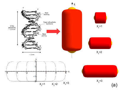
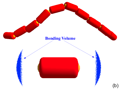
Figure 1: Coarse-grained model of DNA duplexes. (a) DNA duplex and a 3D graphical representation of its corresponding coarse-grained model comprising a SQ, symmetric around the $x$ axis, decorated with two sticky spots located on its bases. The figure also show SQs of different aspect ratios ($X_{0}=1,2,3$) and the projection of their surfaces onto the $xy$-plane. Note that the base roundness increases on increasing $X_{0}$. (b) A random chain of $10$ monomers and a representation (blue clouds) of the points where the center of mass of a different monomer can be located in a bonding configuration. This set of points defines the bonding volume.

II Model and Numerical Details

In this section we introduce a coarse-grained model devised to capture the essential physical features of end-to-end stacking (equilibrium polymerization) of DNA duplexes and well suited to being investigated both theoretically and numerically. In the model, particles (DNADs) are assimilated to superquadrics (SQ) with a quasi-cylindrical shape decorated with two reactive sites on their bases determining their interactions. SQs are a straightforward generalization of hard ellipsoids (HE), their surface is in fact defined as follows:

$$f(x,y,z)=\left|\frac{x}{a}\right|^{p}+\left|\frac{y}{b}\right|^{m}+\left|\frac{z}{c}\right|^{n}-1=0$$ (1)

where the parameters $p,m,n$ are real numbers and $a$, $b$, $c$ are the SQ semi-axes. In our case we set $m=n=2$, $p=16$ and $b=c$, so that the SQ resembles a cylinder with rounded edges (see Fig. 1). Such SQs can be fully characterized by the elongation $X_{0}=a/b$ and by the parameter $p$, that determines the sharpness of the edges (see Fig. 1). SQs of elongation $X_{0}<1$ are called “oblate”, while SQs of elongation $X_{0}>1$ are called “prolate”, as for the HEs. As unit of length in our simulations we use the length of short semi-axes $b$. In the present study we investigated only prolate SQs with elongations $X_{0}=1,2$ and $3$. We chose such elongations because DNADs used in experiments Nakata et al. (2007) have a diameter $D=2nm$ and are composed of $6$ to $20$ base pairs (BP) each $0.3$ nm long, hence their elongation $X_{0}$ ranges from $1$ to $3$.

Each particle is decorated with two attractive sites, located along the symmetry axis ($x$-axis in Fig. 1) at a distance $d/b=X_{0}-0.46$ from the DNAD center of mass, in order to model hydrophobic (stacking) forces between DNADs. Sites belonging to distinct particles interact via the following square-well (SW) potential:

$$\beta u_{\rm SW}\,=\,\begin{cases}-\beta\Delta E_{S}&r<\delta\\ 0&r>\delta\end{cases}\>,$$ (2)

where $r$ is the distance between the interacting sites, $\delta/b=1.22$ is the range of interaction (i.e. the diameter of the attractive sites), $\beta=1/k_{B}T$ and $k_{B}$ is the Boltzmann constant. Therefore in the present model the anisotropic hard-core interaction is complemented with an anisotropic attractive potential in a fashion similar to what has been done in the past for other systems, like water De Michele et al. (2006a), silica De Michele et al. (2006b) and stepwise polymerization of bifunctional diglycidyl ether of bisphenol A with pentafunctional diethylenetriamine Corezzi et al. (2008, 2009).

The location and diameter of the attractive sites have been chosen to best mimic the stacking interactions between blunt-ended DNAD and in particular they ensure that:

1. the maximum interaction range between two DNADs bases is of the order of typical range for hydrophobic interactions (i.e. $2\AA$ see Lee et al. (1984)), i.e. of the order of water molecule dimensions

2. the extent of the attractive surface of the DNADs bases is compatible with the surface of aromatic groups present in DNADs and which are responsible for hydrophobic interactions

We note that in the present model each DNAD is symmetric around the $x-$axis (see Fig. 1), hence we are neglecting rotations around it.

We performed Monte Carlo (MC) simulations in the canonical and isobaric ensembles. We implemented the aggregation biased MC technique (AVBMC) developed by Chen and Siepmann Chen and Siepmann (2000, 2001) in order to speedup the formation of linear aggregates. To detect the overlap of two DNADs we calculated the distance using the algorithm described in Ref. De Michele (2010). In all simulations we adopted periodic boundary conditions in a cubic simulation box. We studied a system of $N=1000$ particles in a wide range of volume fractions $\phi$ and pressure $P$ respectively. Initially we prepared configurations at high temperature with all DNADs not bonded, then we quenched the system to the final temperature (i.e. to the final value of $\beta\Delta E_{S}$) letting the system equilibrate. We checked equilibration by inspecting the behavior of the potential energy and the nematic order parameter (see Sec. V.2) in the system.

III Theory

Following the work of van der Schoot and Cates van der Schoot and Cates (1994a, b) and its extension to higher volume fractions with the use of Parsons-Lee approximation Parsons (1979); Lee (1987) as suggested by Kuriabova et al. T. et al. (2010), we assume the following expression for the free energy of our system:

$$\frac{\beta F}{V} = \sum_{l=1}^{\infty}\nu(l)\left\{\ln\left[v_{d}\nu(l)\right]-1\right\}+$$ (3)

$$+ \frac{\eta(\phi)}{2}\sum_{l=1\atop l^{\prime}=1}^{\infty}\nu(l)\nu(l^{\prime})v_{excl}(l,l^{\prime})$$

$$- (\beta\Delta E_{S}+\sigma_{b})\sum_{l=1}^{\infty}(l-1)\nu(l)+\sum_{l=1}^{\infty}\nu(l)\sigma_{o}(l)$$

where $\nu(l)$ is the number density of chain of length $l$, normalized such that $\sum_{l=1}^{\infty}l\,\nu(l)=\rho$, $v_{d}$ is the volume of a monomer, $\beta\Delta E_{S}$ is the (positive) stacking energy, $v_{excl}(l,l^{\prime})$ is the excluded volume of two chains of length $l$ and $l^{\prime}$ and $\sigma_{b}$ is the entropic free energy penalty for bonding (i.e. is the contribution to free energy due to the entropy which is lost by forming a single bond) and $\eta(\phi)$ is the Parsons-Lee factorParsons (1979)

$$\eta(\phi)=\frac{1}{4}\frac{4-3\phi}{(1-\phi)^{2}}$$ (4)

and $\sigma_{o}$Odijk (1986) accounts for the orientational entropy that a chain of length $l$ loses in the nematic phase (including possible contribution due to its flexibility). Differently from Ref. van der Schoot and Cates (1994b); T. et al. (2010), but as in Ref. Lü and Kindt (2004), we explicitly account for the polydispersity inherent in the equilibrium polymerization using a discrete chain length distribution. We explicitly separate the bonding free energy in an energetic ($\beta\Delta E_{S}$) and entropic ($\sigma_{b}$) contribution. Differently from Ref. van der Schoot and Cates (1994b); Lü and Kindt (2004), but as in Ref. T. et al. (2010) we include the Parson-Lee factor. Indeed, the Parson decoupling approximation satisfactory models the phase diagram of uniaxial hard ellipsoids Camp et al. (1996), hard cylinders Wensink and Lekkerkerker (2009), linear fused hard spheres chains Varga and Szalai (2000), mixtures of hard platelets Wensink et al. (2001a), hard sphero-cylinders Gámez et al. (2010); Cinacchi et al. (2004); McGrother et al. (1996), rod-plate mixtures Wensink et al. (2001b), mixtures of rod-like particlesSzabolcs et al. (2003); Galindo et al. (2003) and mixtures of hard rods and hard spheresCuetos et al. (2007). On the other hand, Ref. Williamson and Jackson (1998) finds that the Parsons theory is not satisfactory in the case of rigid linear chains of spheres.

A justification of the use of Parsons-Lee factor in Eq. (3) for the present case of aggregating cylinders is provided in Appendix A.Here we only note that the present system, in the limit of high $T$ where polymerization is not effective, reduces to a fluid of hard quasi-cylinders, where the use of Parsons-Lee factor is justifiableWensink and Lekkerkerker (2009); Cinacchi et al. (2004); McGrother et al. (1996). Moreover, in the dilute limit ($\eta(\phi)\rightarrow 1$) the excluded volume term in Eq. 3 reduces to the excluded volume of a polydisperse set of cluster with length distribution $\nu(l)$, which is conform to Onsager original theory Onsager (1949). In other words the form chosen in Eq. 3 for the excluded volume contribution to the free energy reduces to the correct expressions in the limit of high temperatures and in that of low volume fractions.

Following Van der Schoot and Cates van der Schoot and Cates (1994a, b) a generic form for $v_{excl}(l,l^{\prime})$ can be assumed as a second order polynomial in $l$ and $l^{\prime}$, with

$$v_{excl}[l,l^{\prime};f({\bf u})]=2\int f({\bf u})f({\bf u}^{\prime})D^{3}\left[\Psi_{1}(\gamma,X_{0})+\right.$$ (5)

$$+ \frac{l+l^{\prime}}{2}\Psi_{2}(\gamma,X_{0})X_{0}+\left.\Psi_{3}(\gamma,X_{0})X_{0}^{2}\;l\,l^{\prime}\right]d{\bf\Omega}\,d{\bf\Omega}^{\prime}$$

where $f({\bf u})$ is the probability for a given monomer of having orientation ${\bf u}$ within the solid ${\bf\Omega}$ and ${\bf\Omega}+d{\bf\Omega}$ and $\Psi_{\alpha}$ describe the angular dependence of the excluded volume. The orientational probability $f({\bf u})$ are normalized as

$$\int f({\bf u})d\Omega=1$$ (6)

In particular for two rigid chains of length $l$ and $l^{\prime}$ which are composed of hard cylinders (HC) of diameter $D$ and length $X_{0}D$ $v_{excl}(l,l^{\prime})$ has been calculated by Onsager in 1949

$$v_{excl}(l,l^{\prime}) = \int f({\bf u})f({\bf u}^{\prime})D^{3}\left[\,\frac{\pi}{2}\sin\gamma+\frac{\pi}{2}X_{0}(1+|\cos\gamma|+\right.$$ (7)

$$+ \left.\frac{4}{\pi}E(\sin\gamma))\frac{l+l^{\prime}}{2}+2X_{0}^{2}\sin\gamma\;\;l\,l^{\prime}\,\right]d{\bf\Omega}\,d{\bf\Omega}^{\prime}$$

where $\cos\gamma={\bf u}\cdot{\bf u}^{\prime}$ and $E(\sin\gamma)$ is the complete elliptical integral

$$E(\sin\gamma)=\frac{1}{4}\int_{0}^{2\pi}(1-\sin^{2}\gamma\sin^{2}\psi)^{1/2}d\psi$$ (8)

On passing we observe that the integrals in Eq. (7) can be calculated exactly in the isotropic phase while in the nematic phase the calculation can be done analytically only with suitable choices of the angular distribution $f({\bf u})$. Comparing Eqs. (7) and (5) for HC one has:

$$\Psi_{1}(\gamma,X_{0}) = \frac{\pi}{2}\sin\gamma$$

$$\Psi_{2}(\gamma,X_{0}) = \frac{\pi}{2}(1+|\cos\gamma|+\frac{4}{\pi}E(\sin\gamma))$$

$$\Psi_{3}(\gamma,X_{0}) = 2\sin\gamma$$ (9)

In view of Eqs. (9) we notice that for HCs the functions $\Psi_{1}(\gamma)$, $\Psi_{2}(\gamma)$ and $\Psi_{3}(\gamma)$ accounts for the orientational dependence of the excluded volume of two monomers having orientations ${\bf u}$ and ${\bf u}^{\prime}$ with ${\bf u}\cdot{\bf u}^{\prime}=\cos\gamma$. It is also worth observing that the first term of the integrand in Eq. (7) is independent of $l$ and hence accounts for the excluded volume interaction between two HCs end caps, the second term is linear in $l$ and $l^{\prime}$ and accounts for the excluded volume between the two end caps of a chain and all midsections of the other one and the third one proportional to $ll^{\prime}$ models the interaction between all $ll^{\prime}$ pairs of midsections of the two chainsvan der Schoot and Cates (1994a, b). In summary, Eq. (5) is exact for two rigid chains of HCs but according to van der Schoot and Cates (1994a); Khokhlov and Semenov (1981) to lowest order of approximation it is justifiable to use such equation also for two semi-flexible chains. We then assume that $v_{excl}$ remains additive with respect to end-end, end-midsection and midsection-midsection excluded volume contributions even if the chain is semi-flexible. Finally our further ansatz is that Eq. (5) is also a good functional form for the excluded volume of two superquadrics having quasi-cylindrical shape: we will check the validity of this hypothesis using our simulations data.

An exact expression for $\sigma_{o}$ is not available. The two following limits have been calculated by Khokhlov and Semenov Khokhlov and Semenov (1982); Odijk (1986); Vroege and Lekkerkerker (1992):

$$\begin{array}[]{llr}\displaystyle\sigma_{o}(l)&\displaystyle=\frac{l}{8l_{p}}\int\left(\frac{df}{d\theta}\right)^{2}f^{-1}d{\bf\Omega}\;+&\\[14.22636pt] &-2\ln\left[\int f^{1/2}d{\bf\Omega}\right]+\ln(4\pi)&\hskip 28.45274pt(l_{p}\ll l)\\[14.22636pt] \displaystyle\sigma_{o}(l)&\displaystyle=\int f\ln(4\pi f)d{\bf\Omega}\;+&\\[14.22636pt] &+\frac{l}{12l_{p}}\int\left(\frac{df}{d\theta}\right)^{2}f^{-1}d{\bf\Omega}&\hskip 28.45274pt(l_{p}\gg l)\end{array}$$ (10)

Finally, we notice that in the limit of rigid rods with $f_{l}({\bf u})=f({\bf u})\nu(l)$, (the same limit selected in Ref. T. et al. (2010)), the free energy in Eq. (3) reduces to:

$$\frac{\beta F}{V} = \frac{2}{3l_{p}}\sum_{l=1}^{\infty}l\int\left[f_{l}({\bf u})\right]^{1/2}\nabla^{2}\left[f_{l}({\bf u})\right]^{1/2}d{\bf\Omega}$$ (11)

$$+ \sum_{l=1}^{\infty}\int f_{l}({\bf u})\left\{\ln\left[4\pi v_{d}f_{l}({\bf u})\right]-1\right\}+$$

$$+ \frac{\eta(\phi)}{2}\sum_{l=1,l^{\prime}=1}^{\infty}\int f_{l}({\bf u})f_{l^{\prime}}({\bf u^{\prime}})v_{excl}d{\bf\Omega}d{\bf\Omega}^{\prime}+$$

$$- (\beta\Delta E_{S}+\sigma_{b})\sum_{l=1}^{\infty}\int(l-1)f_{l}({\bf u})d{\bf\Omega}$$

which is analogous to the free energy expression used by Glaser et al. T. et al. (2010).

III.1 Isotropic phase

In the isotropic phase all orientations are equiprobable, hence:

$$f({\bf u})=\frac{1}{4\pi}$$ (12)

Plugging Eq. (12) into Eq. (3) and calculating the integrals one obtains:

$$\frac{\beta F}{V} = \sum_{l=1}^{\infty}\nu(l)\left\{\ln\left[v_{d}\nu(l)\right]-1\right\}+$$ (13)

$$+ \frac{\eta(\phi)}{2}\sum_{l=1,l^{\prime}=1}^{\infty}\nu(l)\nu(l^{\prime})v_{excl}(l,l^{\prime})+$$

$$- (\beta\Delta E_{S}+\sigma_{b})\sum_{l=1}^{\infty}(l-1)\nu(l)$$

For hard cylinders the excluded volume can be calculated explicitly and it turns out to be:

$$v_{excl}(l,l^{\prime}) = \frac{\pi^{2}}{8}D^{3}+\left(\frac{3\pi}{8}+\frac{\pi^{2}}{8}\right)[l+l^{\prime}]X_{0}D^{3}+$$ (14)

$$+ \frac{\pi}{2}l\,l^{\prime}X_{0}^{2}D^{3}$$

Building on Eq. (14), the generic expression for the excluded volume $v_{excl}(l,l^{\prime})$ reported in Eq. (5) in the isotropic phase takes the form:

$$v_{excl}(l,l^{\prime}) = 2\left[A_{I}(X_{0})+k_{I}(X_{0})v_{d}\frac{l+l^{\prime}}{2}+\right.$$ (15)

$$\left.\phantom{\frac{l+l^{\prime}}{2}}B_{I}(X_{0})X_{0}^{2}ll^{\prime}\right]$$

We assume that the chain length distribution $\nu(l)$ is exponential with a average chain length $M$

$$\nu(l)=\rho M^{-(l+1)}(M-1)^{l-1}$$ (16)

where

$$M=\frac{\sum_{1}^{\infty}l\,\nu(l)}{\sum_{1}^{\infty}\nu(l)}.$$ (17)

With this choice for $\nu(l)$ the free energy in Eq. (13) becomes:

$$\frac{\beta F}{V} = -\rho(\beta\Delta E_{S}+\sigma_{b})(1-M^{-1})+$$ (18)

$$+ \eta(\phi)\left[B_{I}X_{0}^{2}+\frac{v_{d}k_{I}}{M}+\frac{A_{I}}{M^{2}}\right]\rho^{2}+$$

$$+ \frac{\rho}{M}\left[\ln\left(\frac{v_{d}\rho}{M}\right)-1\right]+$$

$$+ \rho\frac{M-1}{M}\ln(M-1)-\rho\ln M.$$

Note that in general $k_{I}$, $B_{I}$ and $A_{I}$ depend on $X_{0}$.

The minimum of the free energy with respect to $M$ (i.e. the equation ${\partial(\beta F/V)}/{\partial M}=0$ provides the searched equilibrium value for $M$. Dropping terms in $O(1/M^{2})$ one obtains

$$M=\frac{1}{2}\left(1+\sqrt{1+4\omega\phi e^{k_{I}\phi\eta(\phi)+\beta\Delta E_{S}}}\right)$$ (19)

where $\omega\equiv 4e^{\sigma_{b}}$. This formula for $M$ differs from the one reported by Kindt Lü and Kindt (2004) by the presence of the Parsons-Lee factor, which will play a role at high volume fractions.

The expression for $M$ in Eq. (19) coincides with the parameter-free expression for average chain length $M_{w}$ obtained within Wertheim’s theory (e.g. see Refs. Wertheim (1984a, b, 1986); Sciortino et al. (2007); Jackson et al. (1988)), when $\phi$ is small and $e^{k_{I}\phi\eta(\phi)}\approx 1$. Indeed, in Wertheim theory

$$M_{W}=\frac{1}{2}+\frac{1}{2}\sqrt{1+8\frac{\phi}{v_{d}}\Delta}$$ (20)

where $\Delta=V_{b}(e^{\beta\Delta E_{S}}-1)$ and $V_{b}$ is the bonding volumeSciortino et al. (2007). In the limit $e^{\beta\Delta E_{S}}\gg 1$, always valid in the $T$-region where chaining takes place,

$$M_{W}=\frac{1}{2}+\frac{1}{2}\sqrt{1+8\frac{V_{b}}{v_{d}}\phi e^{\beta\Delta E_{S}}}$$ (21)

The equivalence between the two expressions provide an exact definition of $\omega$ as

$$\omega=2\frac{V_{b}}{v_{d}}$$ (22)

Although Eq. (19) has been derived ignoring $O(1/M^{2})$ terms in the free energy, the average chain length $M$ can be always calculated, and this is what we do in this work, finding numerically the zero of ${\partial(\beta F/V)}/{\partial M}=0$.

III.2 Nematic Phase

In the nematic phase the function $f({\bf u})$ depends explicitly on the angle between a given particle direction and the nematic axis, i.e. on the axis $\bf u$. The function $f({\bf u})$ is also called the “trial function” and it generally depends on a set of parameters that have to be obtain through the minimization of the free energy. Also in the nematic phase we assume an exponential distribution for $\nu(l)$. In view of the analytical expression for the excluded volume $v_{excl}$ for cylinders, we assume the following form for the $v_{excl}$ of two DNADs averaged over the solid angle using a one parameter ($\alpha$) dependent trial function

$$v_{excl}(l,l^{\prime},\alpha) = 2\left[A_{N}(\alpha)+v_{d}k_{N}(\alpha)\frac{l+l^{\prime}}{2}+\right.$$ (23)

$$\left.\phantom{\frac{l+l^{\prime}}{2}}+B_{N}(\alpha)X_{0}^{2}l\,l^{\prime}\;\right]\hskip 14.22636pt$$

If we insert Eqs. (57), (23) and (16) into Eq. (3) we obtain after some algebra:

$$\frac{\beta F}{V} = \hat{\sigma}_{o}-\rho(\beta\Delta E_{S}+\sigma_{b})(1-M^{-1})+$$ (24)

$$+ \eta(\phi)\left[B_{N}(\alpha)X_{0}^{2}+\frac{k_{N}(\alpha)}{M}v_{d}+\frac{A_{N}(\alpha)}{M^{2}}\right]\rho^{2}+$$

$$+ \frac{\rho}{M}\left(\log\left[\frac{v_{d}\rho}{M}\right]-1\right)-\rho\log M+$$

$$+ \rho\log(M-1)\frac{M-1}{M}$$

where $\hat{\sigma}_{o}\equiv\sum_{l}\sigma_{o}(l)\nu(l)$

III.3 Phase Coexistence

Using the free energy functionals in Eqs. (18) and (24) the phase boundaries, i.e. $\phi_{N}=v_{d}\rho_{N}$ and $\phi_{I}=v_{d}\rho_{I}$, of isotropic-nematic transition can straightforwardly calculated by minimizing the free energy with respect to average chain lengths in the isotropic and nematic phases, i.e. $M_{I}$ and $M_{N}$, and $\alpha$. We also require that the isotropic and nematic phases have the same pressure, i.e. $P_{I}=P_{N}$ and the same chemical potential $\mu_{I}=\mu_{N}$. These conditions require numerically solving the following set of equations:

$$\frac{\partial}{\partial M_{I}}F_{iso}(\rho_{I},M_{I}) = 0$$

$$\frac{\partial}{\partial M_{N}}F_{nem}(\rho_{N},M_{N},\alpha) = 0$$

$$\frac{\partial}{\partial\alpha}F_{iso}(\rho_{I},M_{I},\alpha) = 0$$

$$P_{I}(\rho_{I},M_{I}) = P_{N}(\rho_{N},M_{N},\alpha)$$

$$\mu_{I}(\rho_{I},M_{I}) = \mu_{N}(\rho_{N},M_{N},\alpha)$$ (25)

IV Calculation of free energy parameters

The theory illustrated in the previous section requires the calculation of several parameters, $V_{b}$, $k_{I}$, $A_{I}$, $B_{I}$, $k_{N}$, $A_{N}$, $B_{N}$, $l_{p}$. Since for super-quadrics an explicit calculation of these parameters is very unlikely in the following we describe simple methods to calculate them numerically. For example the calculation of the excluded volume between clusters and the calculation of the bonding volume require the evaluation of complicated integrals, which can be estimated with a Monte Carlo method. The general idea indeed behind Monte Carlo is that such complicated integrals can be calculated by generating a suitable distribution of points in the domain of integration.

IV.1 Excluded volume in the isotropic phase

In the isotropic phase, $v_{excl}(l,l^{\prime})$ can be written as reported in Eq. (15). If $l=l^{\prime}$,

$$v_{excl}(l,l)=2A_{I}+2k_{I}v_{d}\,l+2B_{I}X_{0}^{2}\,l^{2}$$ (26)

Hence, from a numerical evaluation of $v_{excl}(l,l)$ for several $l$ values (whose detailed procedure is described in Appendix X) it is possible to estimate $A_{I}$, $k_{I}$ and $B_{I}$. Fig. 2 shows $v_{excl}(l,l)/l$ vs $l$. A straight line describe properly the data for all $X_{0}$ values, suggesting that $A_{I}\approx 0$. From a linear fit one obtain $2B_{I}X_{0}^{2}$ (slope) and $2k_{I}v_{d}$ (intercept).

Figure 2: (a) Excluded volume of two chains of length $l$ calculated numerically as a function of $l$ for $X_{0}=1,2,3$. Dashed lines are fits to Eq. (26). (b) Bonding volume as a function of elongation $X_{0}$.

IV.2 Calculation of the Bonding Volume

The bonding volume $V_{b}$ can be calculated numerically performing a Monte Carlo calculation of

$$V_{b} = \int\theta\left(-\Delta E_{S}-u_{SW}-V_{HC}\right)\,d{\bf r}\,d{\bf\Omega}_{1}\,{\bf\Omega}_{2}$$ (27)

where $V_{HC}=V_{HC}({\bf r},{\bf\Omega}_{1},{\bf\Omega}_{2})$ is the hard core part of the interaction potential and $\theta(x)$ is the Heaviside step function, i.e. $\theta(x)=1$ if $x\geq 0$ or $0$ otherwise. The detail of the numerical integration are reported in Appendix X. The resulting values of $V_{b}$ for different $X_{0}$ are shown in Fig. 2(b). $V_{b}$ grows with $X_{0}$, an effect introduced by the different rounding of the SQ surface close to the bases. Indeed, how is it shown in Fig. 1, on increasing $X_{0}$ the base surface is more rounded and such different rounding offers a different angular width over which bonds can form, an effect which will also reflect in the $X_{0}$ dependence of the the persistence length of the self-assembled chains, as it will be discussed in details in Sec. IV.5. The dependence of the bonding angle on $X_{0}$ is not present for HCs and in that case the bonding volume would be constant.

IV.3 Nematic phase

In what follows we assume that the angular distribution of the particle orientation can be well described by the one parameter Onsager trial functionOnsager (1949), i.e.:

$$f({\bf u})=f_{O}({\bf u})=\frac{\alpha}{4\pi\sinh\alpha}\cosh(\alpha\cos\theta)$$ (28)

where $\theta$ is the angle between the particle and the nematic axis and the system is supposed to have azimuthal symmetry around such axis. The excluded volume $v_{excl}(l,l,\alpha)$ between two clusters of equal length $l$ can be calculated using the procedure illustrated previously for the isotropic case with the only difference that now monomers are inserted with an orientation extracted from the Onsager angular distribution defined in Eq. (28).

To estimate numerically $A_{N}(\alpha)$, $k_{N}(\alpha)$ and $B_{N}(\alpha)$ we specialize Eq. (23) to the case of $l=l^{\prime}=2$, $l=l^{\prime}=3$, $l=l^{\prime}=4$, evaluating numerically for several values of $\alpha$ $v_{excl}(2,2,\alpha)$, $v_{excl}(3,3,\alpha)$ and $v_{excl}(4,4,\alpha)$. Inverting Eq. (23) allows us to express $A_{N}(\alpha)$, $k_{N}(\alpha)$ and $B_{N}(\alpha)$ as a function of $v_{excl}(2,2,\alpha)$, $v_{excl}(3,3,\alpha)$ and $v_{excl}(4,4,\alpha)$ as explained in detail in Appendix C.

IV.4 Estimate of the orientational entropy in the nematic phase

We propose to model the orientational entropy in the nematic phase using the following expression proposed by Odijk Odijk (1986) (other possibilities can be found in Refs. DuPré and jun Yang (1991) and Hentschke (1990))

$$\hat{\sigma}_{o}^{od} = \sum_{l=1}^{l=\infty}\nu(l)\left\{\ln\alpha+\frac{(\alpha-1)\,l}{6\,l_{p}}\right.$$ (29)

$$+ \left.\frac{5}{12}\ln\left[\cosh\left(\frac{(\alpha-1)\,l}{5\,l_{p}}\right)\right]-\frac{19}{12}\ln 2\right\}$$

This expression, in the limit of “rigid chains” (RC) and “flexible chains” (FC) reduces approximately to the exact limits Khokhlov and Semenov (1981)

$$\begin{array}[]{llr}\displaystyle\sigma_{o}^{RC}(l)&\displaystyle=\log(\alpha)-1+\frac{\alpha-1}{6l_{p}}l&\hskip 28.45274pt\alpha l\ll l_{p}\\ \displaystyle\sigma_{o}^{FC}(l)&\displaystyle=\log(\alpha/4)+\frac{\alpha-1}{4l_{p}}l&\hskip 28.45274pt\alpha l\gg l_{p}\\ \end{array}$$ (30)

Latter formulas can be also obtained plugging the Onsager trial function $f_{O}({\bf u})$ in Eqs. (10).

Unfortunately, Eq. (29) is hardly tractable in the minimization procedure requested to evaluated the equilibrium free energy and hence the two approximations in Eq. (30) are often preferred. While in the case of fixed length polymers, the knowledge of the persistence length selects one of the two expressions, in the case of equilibrium polymers, different chain length will contribute differently to the orientational entropy. In particular, when the chain length distribution is rather wide, it is difficult to assess if the $RC$ (chosen in Ref. T. et al. (2010)) or the $FC$ (chosen in Ref. Lü and Kindt (2004)) limits should be used. To overcome the numerical problem, still retaining both the $RC$ and the $FC$ behaviors, we use the following expression for $\hat{\sigma}_{o}$:

$$\hat{\sigma}_{o} = \sum_{l=1}^{l=l_{0}-1}\nu(l)\left\{\left[\log(\alpha)-1\right]+\phantom{\frac{\alpha-1}{6l_{p}}}\right.$$ (31)

$$+ \left.\frac{\alpha-1}{6l_{p}}\,l\right\}+\sum_{l=l_{0}}^{l=\infty}\nu(l)\left\{\log(\alpha/4)+\frac{\alpha-1}{4l_{p}}\,l\right\}$$

in which the contribution of chains of size $l_{0}$ is treated with the $RC$ while the contribution of longer chains enters with the $FC$ expression. We pick $l_{0}$ by requesting maximum likeihood between Eq. (31) and Eq. (29) in the relevant $M$-$\alpha$ domain. We found that the value $l_{0}\approx 9$ is appropriate for most studied cases.

IV.5 Estimate of persistence length

In order to estimate the persistence length, entering in Eq. (31), we randomly build chains according to the procedure described in Appendix B.We estimate the “chain persistence length” $l_{p}$ by evaluating following spatial correlation function:

$$C_{O}(\left|i-j\right|)\equiv\sum_{i,j}\langle\hat{\mathbb{x}}(i)\cdot\hat{\mathbb{x}}(j)\rangle$$ (32)

where $i,j$ label two monomers along the chain ($i=0$ is the first monomer at chain end) and $\hat{\mathbb{x}}(i)$ is a unit versor directed along $x$-axis of the monomer (i.e. their axis of symmetry, see Fig. 1), that coincides with the direction along which the two attractive sites lie. $\langle\ldots\rangle$ denotes an average over the whole set of independent chains which has been generated.

In Figure 3 we plot $C_{O}(\left|i-j\right|)$ for all elongations studied. All correlations decay following an exponential law, whose characteristic scale is identified as the persistence length (in unit of monomer). In the explored $X_{0}$ range, $10<l_{p}<25$. The more elongated monomers have a smaller persistence length. The $X_{0}$ dependence of $l_{p}$ arises from the different roundness of the bases (implicit in the use of SQ), as discussed in the context of the bonding volume and in Fig. 1.

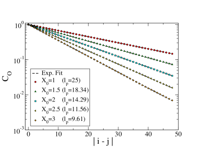
Figure 3: Spatial correlation function $C_{O}(\left|i-j\right|)$ (see text for its definition) calculated generating random chains of $50$ monomers for aspect ratios $X_{0}=1,1.5,2,2.5,3$. Dashed lines are fits to the functional form $C_{O}(\left|i-j\right|)=\exp[-\left|i-j\right|/l_{p}]$. From these fits the chain persistence length $l_{p}$ can be estimated (see legend).

V Results and Discussion

In this section we compare results from simulations with theoretical calculations based on the theory discussed in Sec. III

V.1 Isotropic phase

Fig. 4 (a)-(c) show the packing fraction dependence of $M$ for $X_{0}=1,2,3$ for all temperatures investigated. The dashed curves are calculated by minimizing with respect to $M$ the isotropic free energy in Eq. (18) using the values of $V_{b}$, $k_{I}$ and $B_{I}$ obtained in Sec. IV.1 without any fitting parameter. Up to volume fractions around $\phi\approx 0.20$ the agreement between theoretical and numerical results is quite good for all cases considered. Above such volume fraction the theoretical predictions start deviating appreciably, a discrepancy that we attribute at moderate and high $\phi$ to the inaccuracy of the Parsons decoupling approximation.

In Fig. 4 (d) we report the cluster size distribution $\nu(l)$ as obtained from both simulation and theory, the latter calculated according to Eq. (18) with $M$ obtained by minimization of the isotropic free energy. As expected, the cluster size in the isotropic phase is exponential. These results suggest that a reasonable first principle description of the isotropic phase is provided by the free energy of Eq. (18), when the parameter of the model are properly evaluated.

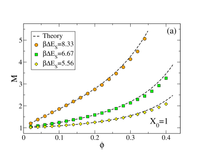
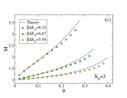
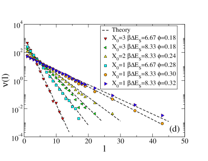
Figure 4: (a)-(c) Average chain length $M$ against $\phi$ for $X_{0}=1,2,3$ at all values of $\beta\Delta E_{S}$ studied. Dashed lines are theoretical predictions calculated by minimizing the free energy in Eq. (18) with values of $V_{b}$, $k_{I}$ and $B_{I}$ derived by the procedure described in Sec. IV. (d) Cluster size distributions (colored symbols) for several state points together with theoretical predictions (dashed lines).

V.2 Nematic phase

On increasing $\phi$ the system transform into a LC phase. We estimate the degree of nematic ordering by evaluating the largest eigenvalue $S$ of the order tensor ${\bf Q}$, whose components are:

$$Q_{\alpha\beta}=\frac{1}{N}\sum_{i}\frac{3}{2}\langle({\bf u}_{i})_{\alpha}({\bf u}_{i})_{\beta}\rangle-\frac{1}{2}\delta_{\alpha,\beta}$$ (33)

where $\alpha\beta\in\{x,y,z\}$, and the unit vector $({\bf u}_{i}(t))_{\alpha}$ is the component $\alpha$ of the orientation (i.e. the symmetry axis) of particle $i$ at time $t$. A non-zero value of $S$ signals the presence of orientational order in the system and it can be found not only in the nematic phase but also in partially ordered phases as columnar and smectic phases. Since in this article we focus only on the nematic phase, to verify that the simulated state points are not partially ordered we calculate, following Ref. T. et al. (2010), the three dimensional pair distribution function $g({\bf r})$ defined as:

$$g({\bf r})=\frac{1}{\rho N}\left\langle\sum_{i=1}^{N}\sum_{j\neq i}\delta({\bf r}-({\bf r}_{i}-{\bf r}_{j}))\right\rangle$$ (34)

where $\delta({\bf x})$ is the Dirac delta function. We calculate the $g({\bf r})$ in a reference system with the $z$-axis parallel to the nematic director. Figure 5 shows $g(x,y,0)$ and $g(0,y,z)$, which correspond respectively to the correlations in a plane perpendicular to the nematic director and in a plane containing it for a given nematic state point ( $X_{0}=2$, $\phi=0.38$, $\beta\Delta E_{S}=8.33)$). The $g(x,y,0)$ is found to be isotropic, ruling out the possibility of a columnar or crystal phase (no hexagonal symmetry is indeed present). The $g(0,y,z)$ reflects the orientational ordering along the nematic direction and rules out the possibility of a smectic phase (no aligned sequence of peaks are presentT. et al. (2010)). Fig. 5(c) shows also a snapshot of the simulated system at the same state point.

In what follows, we have systematically calculated and inspected $g({\bf r})$ to verify that all state points having a value of $S$ large enough to be considered nematic are indeed translationally isotropic, i.e. with no translational order.

(a) (b)      (c)

Figure 5: Plot of $g(x,y,0)$ (a) and $g(0,y,z)$ (b) where the $z$-axis is chosen parallel to the nematic director for $X_{0}=2$, $\phi=0.38$ and $\beta\Delta E_{S}=8.33$. (c) Example of nematic configurations at the same state point.

Fig. 6 shows the nematic order parameter and the average chain length $M$ calculated from simulations as well as with the theoretical methodology described previously for two different elongations at $\beta\Delta E_{S}=8.33$. The theoretical value for $S$ is obtained according to:

$$S(\alpha)=\int 2\pi\frac{3\,\cos^{2}\theta-1}{2}f_{O}(\theta;\alpha)\sin\theta\;d\theta$$ (35)

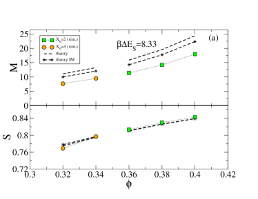
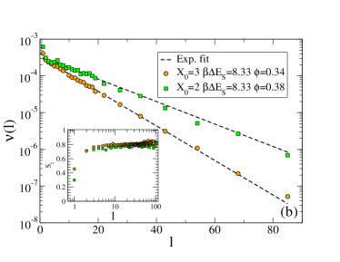
Figure 6: (a) Average chain length and nematic order parameter $S$ for several nematic state points. Dashed lines with stars (theory IM) are theoretical predictions assuming that monomers are isotropic (see text for details). (b) Cluster size distribution for two state points $(X_{0}=2,\phi=0.38,\beta\Delta E_{S}=8.33)$ and $(X_{0}=3,\phi=0.34,\beta\Delta E_{S}=8.33)$. Circles are numerical results and dashed lines are exponential fits. The inset shows the chain length dependent nematic order parameter $S_{l}$ for the same state points.

Fig. 6 (a) shows that the nematic order parameter is very well captured by the theory, while the average chain length shows a clear disagreement between theory and simulations, again suggesting that the error introduced by the Parsons decoupling approximation which was already observed in the isotropic case for large packing fractions is here enhanced by the further increase in $\phi$. Another possible source of error could arise from the hypothesis that the cluster size distribution is exponential also in the nematic phase. To test this hypothesis we show in Fig. 6 (b) the cluster size distributions in two different state points. In all cases, the distributions are not a single exponential. This phenomenon has been already observed and discussed by Lu and Kindt Lü and Kindt (2004) and described as a two exponential decay of $\nu(l)$ with the exponential decay of short chains extending up to $l\approx 50$. They took into account such bi-exponential nature of the distribution to better reproduce the isotropic-nematic phase boundaries Lü and Kindt (2006) in their theoretical approach. In the present case, only very short chains (not to say only the monomers), fall out of the single exponential decay. To test if the different decay reflects a different orientational ordering of the small clusters compared to long chains, we follow Ref. Lü and Kindt (2006) and evaluate the length-dependent nematic order parameter $S_{l}$, that is the nematic order parameter calculated for each population of clusters of size $l$. The results, reported in the inset of Fig. 6(b), show that $S_{l}$ is around $0.7-0.8$ for all clusters sizes except for $l=1$, i.e. except for monomers.

To assess how much the theoretical predictions are affected by the assumption of a single exponential decay (and of the associated identity of $S$ for all chains), we evaluate the correction of the free energy functional in Eq. (24) arising from the assumption that monomers are isotropic, while all other chains are nematic. To do so we exclude from the calculation of the orientational entropy the monomers and take into account in the calculation of the excluded volume contribution the fact that monomers are isotropic. The revised free energy can be thus written as

$$\frac{\beta F}{V} = \hat{\sigma}_{o}^{*}-\rho(\beta\Delta E_{S}+\sigma_{b})(1-M^{-1})+$$

$$+ \eta(\phi)\left[B_{N}(\alpha)X_{0}^{2}+\frac{k_{N}(\alpha)}{M}v_{d}+\frac{A_{N}(\alpha)}{M^{2}}\right]\rho^{2}+$$

$$- \beta\Delta f_{N}+\frac{\rho}{M}\left(\log\left[\frac{v_{d}\rho}{M}\right]-1\right)-\rho\log M+$$

$$+ \rho\log(M-1)\frac{M-1}{M}$$

where

$$\sigma_{o}^{*} = \sum_{l=2}^{l=l_{0}-1}\nu(l)\left\{\left[\log(\alpha)-1\right]+\frac{\alpha-1}{6l_{p}}\,l\right\}+$$ (37)

$$+ \sum_{l=l_{0}}^{l=\infty}\nu(l)\left\{\log(\alpha/4)+\frac{\alpha-1}{4l_{p}}\,l\right\}$$

and

$$\beta\Delta f_{N} = \eta(\phi)\left\{v_{d}[k_{N}(\alpha)-k_{I}]\left(\frac{1}{M^{2}}+\frac{1}{M^{3}}\right)+\right.$$ (38)

$$+ \left.2X_{0}^{2}[B_{N}(\alpha)-B_{I}]\frac{1}{M^{2}}+2\frac{A_{N}(\alpha)}{M^{3}}\right\}\rho^{2}$$

Minimizing such expression we calculate the resulting improved estimate for the average chain length and nematic order parameter and the results are also shown in Fig. 6. The new estimates slightly improve over the previous ones, suggesting once more that the leading source of error in the present approach, as well in all previous, has to be found in the difficulty of properly handling the term successive to the second in the virial expansion.

V.3 Phase Coexistence

NPT-MC simulations provide a rough estimate of the location of phase boundaries, being affected by the hysteresis associated to the metastability of the coexisting phases. It is possible thus only to bracket the region of coexistence, by selecting the first isotropic state point on expansion runs which started from a nematic configuration and the first nematic state point on compression runs started from an isotropic configuration. We performed NPT-MC simulations for $X_{0}=2$ and $\beta\Delta E_{S}=6.67$ in a wide range of pressures $P$ for a system of $1000$ SQs. The resulting equation of state is shown in Fig. 7(a). As expected a clear hysteresis is observed, which allows us to detect some overestimated boundaries for the isotropic-nematic transition. The same figure also reports the theoretical estimates of the transition. The theoretical critical pressure is smaller than the numerical one, resulting into a extended region of coexistence then numerically observed. Comparing the values of the pressure predicted by the theory with the simulation values, we notice that the main error arises from the pressure of the nematic phase which is underestimated. Finally, Fig. 7 (b)-(d) show the predicted phase diagram for several values of $\beta\Delta E_{S}$ as a function of the elongation. On increasing $\beta\Delta E_{S}$ (i.e. decreasing $T$ or increasing the stacking energy) there is a small decrease of $\phi_{I}$ and a significant decrease of $\phi_{N}$, resulting in an overall decrease of the $I-N$ coexistence region. Such trend can be understood in term of increase of the average chain length resulting from the increase of $\beta\Delta E_{S}$. As expected, both $\phi_{I}$ and $\phi_{N}$ decrease on increasing $X_{0}$.

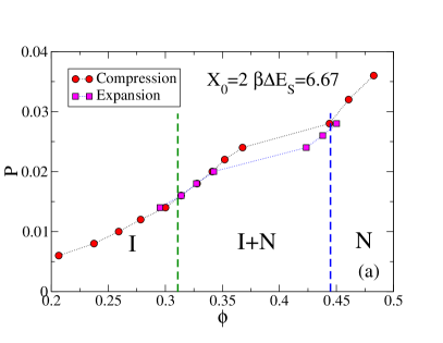
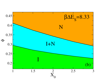
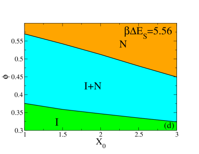
Figure 7: (a) Equation of state ($P$ vs $\phi$) calculated compressing an isotropic initial configuration (squares) or expanding an initial nematic configurations (circles). Vertical dashed lines show the theoretical predictions for the phase boundaries. (b)-(d) Coexistence regions predicted from theoretical calculations for the $3$ stacking energies values $\beta\Delta E_{S}$ investigated.

Finally we recall that in our model the persistence length $l_{p}$ depends on the elongation as discussed in Section IV.5, anyway the dependence on $l_{p}$ of the theoretical phase diagrams showed in Fig. 7 (b)-(d) is negligible at the present level of accuracy of our theoretical calculations.

VI Comparison with experiments

Refs. Nakata et al. (2007) and Zanchetta et al. (2010) report the critical concentrations ($c$), in $mg/ml$, for the $I-N$ transition of blunt-ended DNAD. These experimental data can be transformed into volume fractions once the relevant properties of DNAD are known (DNAD molecular weight $m_{D}=660\,N_{b}$, diameter $D\approx$ $2\;nm$, length $L=N_{b}/3\;nm$, where $N_{b}$ is the number of bases in the sequence). The number density $\rho$ of DNADs is related to the mass concentration

$$\rho=\frac{c}{Nm_{D}}$$ (39)

Since $v_{d}=LD^{2}\pi/4$ is the volume of a DNAD, the volume fraction can be expressed as:

$$\phi=\rho v_{d}=\frac{cLD^{2}\pi}{4Nm_{D}}$$ (40)

Data in Refs. Nakata et al. (2007) and Zanchetta et al. (2010) put in evidence that blunt-end duplexes of equal length but different sequences may have different transition concentrations. As discussed in Ref. Zanchetta et al. (2010) this phenomenon can be attributed to the slight differences in B-DNA helical conformation resulting from the difference in sequences. These differences induce some curvature in the DNAD aggregates, in turn enhancing the transition concentration. Indeed, sequences that are known to form straight double helices order into the $N$ phase at lower concentrations. Therefore, for each oligomer length in the range $8$-$16$ bases, we selected the lowest transition concentration among the ones experimentally determined, since these would be relative to duplexes closest to the symmetric monomers considered in the model. Such values have been reported in Figure 8 as a function of base number $N_{b}$ (top axis) and as a function of $X_{0}$ (bottom axis). Apart for $N_{b}=12$, of which a large number of sequences have been studied, the transition concentrations for the other $N_{b}$ values would probably be corrected to lower values if a larger number of sequences were experimentally explored. We would expect this to be particularly true for the shortest sequences, in which the effect of bent helices could be more relevant.

In the experiments, DNADs are in a water solution with counter-ions resulting from the dissociation of the ionic groups of the phosphate-sugar chain. Given the high DNA concentration necessary for the formation of the $N$ phase, corresponding to concentration of nucleobases in the $1M$ range, the ionic strength simply provided by the natural counter-ions is large enough to effectively screen electrostatic interactions between DNADs. This becomes less true for the longest studied sequences, for which the transition concentration is lower. We hence decided to perform a small number of test experiments on the $N_{b}=20$ oligomers with a double purpose: (i) determine more accurately the transition concentration value for this compound and (ii) test the effect of varying the ionic strength predicted by the model here described. With respect to a fully screened DNAD where electrostatic repulsion can be neglected, a partly screened DNAD has a larger effective volume, thus filling a larger volume fraction of the solution, and a smaller axial ratio $X_{0}$, since electrostatic repulsion is equal in all directions. Therefore, adding salt would bring about two competing effects: the reduction in particle volume enhances the concentration needed to reach the $I-N$ phase boundary, while the grown of $X_{0}$ could favor the nematic ordering even at lower concentrations.

In particular according to Eq. (40) the following relation between the critical concentration $c_{N}$ and the critical volume fraction $\phi_{N}$ holds:

$$c_{N}=\phi_{N}(X_{0})\frac{4Nm_{D}}{LD^{2}}$$ (41)

On the basis of the phase diagrams of Figure 7 (b)-(d) $\phi_{N}(X_{0})$ depends weakly on $X_{0}=L/D$, i.e. $\phi_{N}(X_{0})\approx\phi_{N}^{0}$, where $\phi_{N}^{0}$ is a constant. Hence the theory introduced in the present paper predicts that a reduction of DNAD effective volume due to the addition of salt (i.e. a decrease of $LD^{2}$ in Eq. (41) leads to an overall increase of the concentration required for $N$ ordering.

We have measured the transition concentration of the self-complementary $20$mer $CGCGAAAATTTTCGCG$, a sequence whose $I-N$ transition at room temperature was previously measured and determined to be $c_{IN}\approx$ 200 $mg/ml$ Nakata et al. (2007). With the same method, based on the measurement of the refractive index of the solution, we determined the $I-N$ transition concentration at room temperature at three different ionic strengths. The values we obtained are $c_{IN}\approx 215\,mg/ml$ (no added salt), $c_{IN}\approx 320\,mg/ml$ ($0.8$ M NaCl), $c_{IN}\approx 380\,mg/ml$ ($1.2$ M NaCl). The data indicate that the onset of the nematic ordering in solutions of $20$mers is indeed sensitive to the ionic strength, and that the transition concentration grows upon increasing the amount of salt, as expected on the basis of our theoretical calculations for the present model. In Figure 8 we display the transition volume fraction derived by the transition concentration measured for $1.2$ M NaCl. At this ionic strength, the total concentration of Na⁺ (dissociated from the oligomers + added with the salt) is about the same as the one resulting from counterions dissociated oligomers in the more concentrated solutions of shorter ($8$-$12$ mers) oligomers.

Figure 8 compares the experimentally determined transition volume fractions with the values calculated from the model for $\beta\Delta E_{S}=6.67$ and $\beta\Delta E_{S}=5.56$. Although experimental data are noisy, they fall in the range $\Delta E_{S}\approx 5-7$ (in units of $k_{B}T$). Despite all the simplifying assumptions and despite the experimental uncertainty, results in Figure 8 provide a reasonable description of the $X_{0}$ dependence of $\phi_{N}$.

In comparing the model with the experimental results, it is necessary to take note of the fact that the stacking energy between nucleobases, and thus the interaction energy $\Delta E_{S}$ between DNAD, is temperature dependent, i.e. its entropic component is relevant Bellini et al. (2011). This is a general property of solvation energies and thus it is in line with the notion that stacking forces are mainly of hydrophobic nature. Therefore, the range of values for $\Delta E_{S}$ determined in Figure 8 should be compared to the values of $\Delta G$ for the stacking interactions at the temperature at which the experiments were performed. Overall, the estimate of $\Delta E_{S}$ here obtained appears as in reasonable agreement with the free energies involved in the thermodynamic stability of the DNA double helices and confirms the rough estimate that was given before (see the supporting online material associated to Ref. Nakata et al. (2007)).

Figure 8: Critical volume fractions $\Phi_{N}$ as a function of elongation $X_{0}$ (or equivalently $N_{b}$) from theoretical calculations (for $\beta\Delta E_{S}=6.67$ and $\beta\Delta E_{S}=5.56$) and experimentsNakata et al. (2007) (circles).

.

VII Conclusions

In this study we have developed a free energy functional in order to calculate the phase diagram of bi-functional quasi-cylindrical monomers, aggregating into equilibrium chains, with respect to isotropic-nematic transition. The model has been inspired by experiments on the aggregation of short DNA which exhibit at sufficiently high concentration nematic phases and the comparison between the theoretical predictions and the experimental results allows us to provide an estimate of the stacking energy, consistent with previous propositions.

Our approach is quite general, parameter free and not restricted to particular shapes. We provide techniques to evaluate the bonding volume and the excluded volume, which enters into our formalism via the Parson-Lee decoupling approximation. We build on previous work, retaining the discrete cluster size description of Ref. Lü and Kindt (2004) and the Parson-Lee factor for the excluded volume contribution proposed in Ref. T. et al. (2010). With respect to previous approaches we (i) explicitly account for the entropic and energetic contributions associated to bond formation; (ii) we do not retain any adjustable fit parameter.

The resulting description of the isotropic phase is rather satisfactory and quantitative up to $\phi\approx 0.2$. The description of the nematic phase partially suffers from some of the approximations made in deriving the free energy functional. More specifically, several signatures point toward the failure of the Parsons decoupling approximation in the $\phi$ range typical of the nematic phase. While there is a sufficient understanding of the quality of such approximation for monodisperse object Wensink and Lekkerkerker (2009); Cinacchi et al. (2004); McGrother et al. (1996); Wensink et al. (2001a); Camp et al. (1996); Cuetos et al. (2007), work need to be done to assess the origin of the failure of this approximation in the equilibrium polymer case and to propose improvements.

We finally remind that the model here introduced does not consider the azimuthal rotations of each monomer around its axis. This neglect is adequate when the aggregation does not entail constraints in the azimuthal freedom of the monomers. This is the case of base stacking, in which the angular dependence of the stacking energy is arguably rather small. However, this is not the case of DNAD interacting through the pairing of overhangs and of the LC ordering of RNA duplexes. Because of its A-DNA-type structure, the terminal paired bases of RNA duplexes are significantly tilted with respect to the duplex axis, thus establishing even in the case of blunt-ended duplexes a link between the azimuthal angle of the aggregating duplexes and the straightness of the aggregate. However, with minor modifications the model here introduced could become suitable to include these additional situations. The limiting factor in developing such extension is the lack of knowledge to quantify the azimuthal constraints implied by these interactions. This situation, as well as the effects of off-axis components of the end-to-end interduplex interactions, will be explored in a future work.

VIII Acknowledgments

CDM and FS acknowledge support from ERC (226207-PATCHYCOLLOIDS).

IX Appendix A

Here we provide a justification for the use of Parsons decoupling approximation in the case of linear chains poly-disperse in length (with distribution $\nu(l)$), based on the extension of Onsager’s second-virial theory to mixtures of non-spherical hard bodies proposed in Ref. Malijevskí et al. (2008). The contribution $F_{excl}$ to the free energy due to excluded volume interactions between chains can be written if we neglect intrachain interactions Honnell et al. (1987); Malijevskí et al. (2008):

$$\frac{\beta F_{excl}}{V} = \frac{\rho}{6}\int_{0}^{\rho}d\rho^{\prime}\int d{\bf r}\int d{\bf\Omega}_{1}d{\bf\Omega}_{2}\sum_{ll^{\prime}}\frac{\nu(l)\nu(l^{\prime})}{{\rho}^{2}}$$ (42)

$$g_{ll^{\prime}}({\bf r},{\bf\Omega}_{1},{\bf\Omega}_{2})f({\bf\Omega}_{1})f({\bf\Omega}_{2})\,{\bf r}\cdot\nabla_{\bf r}V_{HC}({\bf r},{\bf\Omega}_{1},{\bf\Omega}_{2})$$

where ${\bf r}$ is the distance between the centers of mass of the two chains $1$ and $2$, ${\bf\Omega}_{1}=\{{\bf u}_{1}^{1},\ldots{\bf u}_{l}^{1}\}$ and ${\bf\Omega}_{2}=\{{\bf u}_{1}^{2},\ldots{\bf u}_{l^{\prime}}^{2}\}$ are the orientations of the two chains, where ${\bf u}_{i}^{\alpha}$ is the orientation of monomer $i$ belonging to chain $\alpha=1,2$, $g_{ll^{\prime}}({\bf r},{\bf\Omega}_{1},{\bf\Omega}_{2})$ is the molecular radial distribution function of the mixture, which represents the correlations between two chains of length $l$ and $l^{\prime}$, whose relative distance is ${\bf r}$ and which have orientations ${\bf\Omega}_{1}$ and ${\bf\Omega}_{2}$ respectively, $V_{HC}({\bf r},{\bf\Omega}_{1},{\bf\Omega}_{2})$ is the hard-core part of the interaction potential and $f({\bf\Omega}_{\alpha})$ is the angular distribution function of chain $\alpha$. We note that in Eq. (42) the integration in $\rho^{\prime}$ is performed keeping fixed all the parameters related to $f({\bf\Omega}_{\alpha})$. Neglecting intra-chain interactions is equivalent to ignore self-overlaps of chains, an assumption which is appropriate if chain length is not much greater than its persistence length and the chains can be considered non-extensible.

Parsons decoupling approximations in this case accounts to putting:

$$g_{ll^{\prime}}({\bf r},{\bf\Omega}_{1},{\bf\Omega}_{2})=g^{HS}_{ll^{\prime}}[r/\sigma_{ll^{\prime}}(\hat{r},{\bf\Omega}_{1},{\bf\Omega}_{2})]$$ (43)

where $g^{HS}_{ll^{\prime}}$ is the radial distribution function of a mixture of hard spheres and $\sigma_{ll^{\prime}}(\hat{r},{\bf\Omega}_{1},{\bf\Omega}_{2})$ is an angle-dependent range parameter which depends on chain lengths $l$ and $l^{\prime}$. If the pair interaction is of the special form

$$V_{HC}({\bf r},{\bf\Omega}_{1},{\bf\Omega}_{2})=V_{HC}[r/\sigma_{ll^{\prime}}(\hat{r},{\bf\Omega}_{1},{\bf\Omega}_{2})]$$ (44)

noting that ${\bf r}\cdot\nabla_{\bf r}=r\frac{\partial}{\partial r}$, Eq. (42) becomes:

$$\frac{\beta F_{excl}}{V} = \frac{\rho}{6}\int_{0}^{\rho}d\rho^{\prime}\int d\hat{r}\,d{\bf\Omega}_{1}\,d{\bf\Omega}_{2}\sum_{ll^{\prime}}\frac{\nu(l)\nu(l^{\prime})}{{\rho^{\prime}}^{2}}$$ (45)

$$\int dr\;r^{3}g^{HS}_{ll^{\prime}}(r/\sigma_{ll^{\prime}})f({\bf\Omega}_{1})f({\bf\Omega}_{2})\,\frac{\partial\,V_{HC}(r/\sigma_{ll^{\prime}})}{\partial r}$$

With the substitution $y=r/\sigma_{ll^{\prime}}$ from Eq. (45) one obtains:

$$\frac{\beta F_{excl}}{V} = \frac{\rho}{2}\sum_{ll^{\prime}}\frac{1}{3}\frac{\nu(l)\nu(l^{\prime})}{{\rho}^{2}}\int_{0}^{\rho}d\rho^{\prime}\int d\hat{r}\,d{\bf\Omega}_{1}\,d{\bf\Omega}_{2}$$ (46)

$$\int dy\;y^{3}\frac{\partial V_{HC}(y)}{\partial y}g^{HS}_{ll^{\prime}}(y)f({\bf\Omega}_{1})f({\bf\Omega}_{2})\sigma_{ll^{\prime}}^{3}$$

The derivative of $V_{HC}$ is a delta function hence we need only to evaluate the value of $g^{HS}_{ll^{\prime}}(y)$ at contact (i.e. $y=1^{+}$) and Eq. (46) becomes:

$$\frac{\beta F_{excl}}{V} = \frac{\rho}{2}\sum_{ll^{\prime}}\frac{\nu(l)\nu(l^{\prime})}{{\rho}^{2}}\int d\rho^{\prime}g_{ll^{\prime}}^{HS}(1^{+})\int d\hat{r}\,d{\bf\Omega}_{1}\,d{\bf\Omega}_{2}f({\bf\Omega}_{1})f({\bf\Omega}_{2})\frac{\sigma_{ll^{\prime}}^{3}}{3}$$

This expression tends to Parson’s expression when the system is monodisperse ($\nu(l)=\rho\delta_{l,1}$). In the specific case of spherical particles $\sigma_{ll^{\prime}}(\hat{r},{\bf\Omega}_{1},{\bf\Omega}_{2})=\sigma(\hat{r},{\bf\Omega}_{1},{\bf\Omega}_{2})=\sigma$ and

$$\sum_{ll^{\prime}}\nu(l)\nu(l^{\prime})f({\bf\Omega}_{1})f({\bf\Omega}_{2})\int d\hat{r}\,d{\bf\Omega}_{1}\,d{\bf\Omega}_{2}\frac{1}{3}\sigma(\hat{r},{\bf\Omega}_{1},{\bf\Omega}_{2})=\frac{4\pi}{3}\sigma^{3}$$ (47)

i.e. the excluded volume of two spheres of diameter $\sigma$. Hence we are allowed to make the identification:

$$v_{excl}(l,l^{\prime}) = \int d\hat{r}\,d{\bf\Omega}_{1}\,d{\bf\Omega}_{2}\frac{1}{3}f({\bf\Omega}_{1})f({\bf\Omega}_{2})\sigma_{ll^{\prime}}^{3}(\hat{r},{\bf\Omega}_{1},{\bf\Omega}_{2})$$ (48)

and write:

$$\frac{\beta F_{excl}}{V}=\frac{\rho}{2}\sum_{ll^{\prime}}\frac{\nu(l)\nu(l^{\prime})}{{\rho}^{2}}\left[\int d\rho^{\prime}g_{ll^{\prime}}^{HS}(1^{+})\right]v_{excl}(l,l^{\prime})$$ (49)

We note that the identification made in Eq. (48) can be also further justified using the same reasonings given in Sec. III. As discussed in Ref. Malijevskí et al. (2008) a possible expression for $g_{ll^{\prime}}^{HS}$ is the one derived by Boublík Boublík (1970), which generalizes the Carnahan–Starling relation Carnahan and Starling (1969) for pure hard spheres to the case of mixtures, i.e.

$$g^{HS}_{ll^{\prime}}(1^{+})=\frac{1}{1-\zeta_{3}}+\frac{3\,\zeta_{2}}{(1-\zeta_{3})^{2}}\frac{\hat{\sigma}_{ll}\hat{\sigma}_{l^{\prime}l^{\prime}}}{\hat{\sigma}_{ll}+\hat{\sigma}_{l^{\prime}l^{\prime}}}+\frac{2\,\zeta_{2}^{2}}{(1-\zeta_{3})^{3}}\frac{\left(\hat{\sigma}_{ll}\hat{\sigma}_{l^{\prime}l^{\prime}}\right)^{2}}{(\hat{\sigma}_{ll}+\hat{\sigma}_{l^{\prime}l^{\prime}})^{2}}$$ (50)

where $\hat{\sigma}_{ll}$ is the diameter of an hard sphere corresponding to a chain of length $l$ and $\zeta_{n}=(\pi/6)\sum_{l}\nu(l)\hat{\sigma}_{ll}^{n}$. To map the system of polydisperse chains onto the equivalent mixture of hard spheres we need an expression for $\hat{\sigma}_{ll}$. According to Ref. Malijevskí et al. (2008), the simplest choice is to consider spheres having the same volume of the corresponding linear chain of length $l$, i.e.

$$v_{d}=\frac{\pi}{6\,l}\hat{\sigma}_{ll}^{3}$$ (51)

where we recall that $v_{d}$ is the volume of a monomer. Although in principle we could use Eq. (49) together with Eqs. (50) and (51) to calculate the free energy contribution due to the excluded volume between particles, if we make the further assumption that

$$g_{ll^{\prime}}^{HS}(1^{+})\approx g^{HS}(1^{+})$$ (52)

i.e. if we approximate the radial distribution function of the hard spheres mixture at contact with that of a monodisperse system of hard spheres having the same total volume fraction (i.e. setting in Eq. (50) $\hat{\sigma}_{ll^{\prime}}=\hat{\sigma}$ with $Mv_{d}=(\pi/6)\sigma^{3}$), we finally obtain

$$\frac{\beta F_{excl}}{V}=\frac{\eta(\phi)}{2}\sum_{ll^{\prime}}\nu(l)\nu(l^{\prime})v_{excl}(l,l^{\prime})$$ (53)

where we used the Carnahan-Starling expression for $g^{HS}(1^{+};\rho^{\prime})$ and we performed the integration in $\rho^{\prime}$. Eq. (53) is exactly the expression for the contribution to the free energy due to steric repulsion which we used in Section III. In summary according to the above derivation we argue that Eq. (53) can be not accurate at high volume fractions due to the approximations made in Eqs. (43) (i.e. the Parsons decoupling approximation) and (52). Within the present treatment Eq. (53) is also not appropriate for chains with $l\gg l_{p}$ because, as already noted, chain self-overlaps can be significant and the hard body pair potential $V_{HC}$ does not have the special form assumed in Eq. (44).

We finally note that the approximation made in Eq. (52) can be avoided if one resorts to Eq. (49) instead of Eq. (53), although the required free energy calculations would become much more complicated. Anyway we verified for the isotropic phase that employing Eq. (49) instead of Eq. (52) does not provide any appreciable improvement in the present case.

X Appendix B

The procedure to calculate the excluded volume $v_{excl}$ in the isotropic phase consists in performing $N_{att}$ attempts of inserting two chains of length $l$ in a box of volume $V$ as described in the following:

1. Set the counter $N_{ov}=0$

2. Build first chain of length $l$ randomly, according to the following procedure:

   1. Insert a first randomly oriented monomer.

   2. Insert a monomer $\cal M$ bonded to a free site $\cal S$ on chain ends ($\cal S$ can be chosen randomly among the two free sites of the partial chain). The orientation of $M$ will be random and its position will be chosen randomly within the available bonding volume between $\cal M$ and $\cal S$. The bonding volume between $\cal M$ and $\cal S$ is defined as the volume corresponding to all possible center of mass positions of $\cal M$ with $\cal M$ bonded to $\cal S$.

   3. If the number of monomer inserted is $l$ terminate otherwise go to 1).

   where the first monomer inserted is placed in the center of the box and it is oriented with its attractive sites parallel to the $x$-axis.

3. Build a second chain of length $l$, where the first monomer inserted is placed randomly within the simulation box with a random orientation.

4. Increase $N_{ov}$ by $1$ if two monomers belonging to different chains overlap and the two chains are either not self-overlapping or forming a closed loop.

5. if the number of attempts is less than $N_{att}$ go to 2) otherwise terminate.

Then $v_{excl}$ can be calculated as follows:

$$v_{excl}=\frac{N_{ov}}{N_{att}}V$$ (54)

A reasonable choice for the total number of attempts is $N_{att}=10^{6}$. In a similar fashion one can also calculate the bonding volume Sciortino et al. (2007) between two monomers. In this case one monomer is kept fixed in the center of the simulation box and the other one is inserted with random position and orientation for a total of $N_{att}$ attempts. The bonding volume will be:

$$V_{b}=\frac{N_{bond}}{4N_{att}}V$$ (55)

where the factor $4$ accounts for the fact that two particles can form $4$ different possible bonds and $N_{bond}$ is the number of times that the two monomers were bonded after a random insertion. Finally with the same procedure used to calculate the excluded volume in the isotropic phase we can evaluate the excluded volume in the nematic phase. The only difference is that now monomers have to be inserted with an orientation extracted from the Onsager angular distribution defined in Eq. (28), so that the excluded volume depends also on the parameter $\alpha$. Again if $N_{ov}$ is the number of times that two monomers belonging to different clusters overlap and $N_{att}$ is the total number of attempts then we have:

$$v_{excl}(l,l,\alpha)=\frac{N_{ov}}{N_{att}}V$$ (56)

XI Appendix C

In this Appendix we explain how to calculate the parameters $A_{N}(\alpha)$, $k_{N}(\alpha)$ and $B_{N}(\alpha)$ of the nematic free energy functional. As a preliminary step we check that $v_{excl}(l,l^{\prime},\alpha)$ for a fixed value of $\alpha$ is a second order polynomial of $l$ and $l^{\prime}$ as assumed in Eq. (5). In Fig. 9 (a) we plot $v_{excl}(l,l,\alpha)$ as a function of $l$ for different values of $\alpha$ and $X_{0}$, $v_{excl}(l,l,\alpha)$ can be well represented by a parabolic function, in agreement with Eq. (5).

We start by observing that the $\alpha$ dependence of $A_{N}(\alpha)$, $k_{N}(\alpha)$ and $B_{N}(\alpha)$ in the case of hard cylinders following the Onsager distribution can be expanded in powers of $\alpha^{-1/2}$ as

$$A_{N}(\alpha) = c_{00}+\frac{c_{01}}{\alpha^{1/2}}+\frac{c_{02}}{\alpha}+\frac{c_{03}}{\alpha^{3/2}}+\frac{c_{04}}{\alpha^{2}}$$

$$k_{N}(\alpha) = c_{10}+\frac{c_{11}}{\alpha^{1/2}}+\frac{c_{12}}{\alpha}+\frac{c_{13}}{\alpha^{3/2}}+\frac{c_{14}}{\alpha^{2}}$$

$$B_{N}(\alpha) = c_{20}+\frac{c_{21}}{\alpha^{1/2}}+\frac{c_{22}}{\alpha}+\frac{c_{23}}{\alpha^{3/2}}+\frac{c_{24}}{\alpha^{2}}$$ (57)

where $c_{ij}$ are the elements of the $3\times 4$ matrix $\bf C$. In the case of cylinders, some of the $c_{ij}$ vanishesOdijk (1986). We assume here that the same $\alpha$ dependence holds for SQ.

In view of this result the co-volume as function of $l$ and $\alpha$ can be expressed as

$$v_{excl}^{(fit)}(\alpha;X_{0},l)=d_{l0}+\frac{d_{l1}}{\alpha^{1/2}}+\frac{d_{l2}}{\alpha}+\frac{d_{l3}}{\alpha^{3/2}}+\frac{d_{l4}}{\alpha^{2}}$$ (58)

where $d_{l,p}$, for $p=0,4$ are fitting parameters. Fig.9 (b)-(d) shows the numerical calculation of the covolume varying $\alpha$ for three particular elongations ($X_{0}=1,2,3$), together with fits to the functional form of Eq. (58).

The good quality of the fits (reduced $\chi^{2}$ is always much less than $1$ for all fits) suggests that retaining terms up to $O(1/\alpha^{2})$ is to the present level of accuracy of our calculations absolutely appropriate.

From these fits we can estimate the matrix $\bf C$ needed to evaluate the free energy in the nematic phase for each $X_{0}$. If we define in fact the following matrix $\bf P$ and the vectors ${\bf q}_{p}$, with $p=0\ldots 4$ as follows:

$${\bf P}=\left(\begin{matrix}1&l_{a}&l_{a}^{2}\\ 1&l_{b}&l_{b}^{2}\\ 1&l_{c}&l_{c}^{2}\end{matrix}\right)\;\;{\bf q}_{p}=\left(\begin{matrix}d_{l_{a}p}\\ d_{l_{b}p}\\ d_{l_{c}p}\end{matrix}\right)$$ (59)

where $l_{a}$, $l_{b}$ and $l_{c}$ are three different chain lengths for which we calculated the $v_{excl}$ as a function of $\alpha$, then we can calculate the matrix elements of $\bf C$ in the following way:

$$2\left(\begin{matrix}c_{0p}\\ v_{d}c_{1p}\\ X_{0}^{2}c_{2p}\end{matrix}\right)={\bf P}^{-1}{\bf q}_{p}.$$ (60)

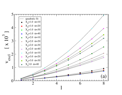
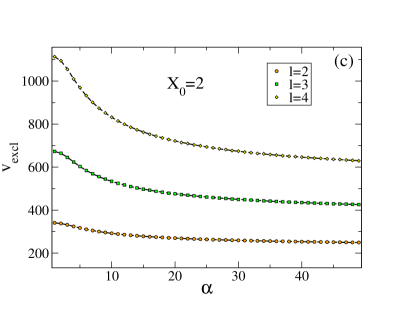
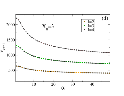
Figure 9: (a) Excluded volume of two chains of length $l$ as a function of chain length for the nematic cases $\alpha=10,20,30,40$ and three different elongations $X_{0}=1,2,3$. (b)-(d) Excluded volume in the nematic phase calculated numerically as a function of $\alpha$ for two chains of equal length $l$, where $l=2,3,4$, composed of monomers with $X_{0}=1,2,3$.

References

- Hamley (2007) I. Hamley, Introduction to Soft Matter (Wiley & Sons, 2007).
- Glotzer (2004) S. C. Glotzer, Science 306, 419 (2004).
- Whitesides and Boncheva (2002) G. M. Whitesides and M. Boncheva, Proceedings of the National Academy of Sciences 99, 4769 (2002).
- Workum and Douglas (2006) V. Workum and J. Douglas, Phys. Rev. E 73, 031502 (2006).
- Mirkin et al. (1996) C. Mirkin, R. Letsinger, R. Mucic, and J. Storhoff., Nature 382, 607 (1996).
- Manoharan et al. (2003) V. N. Manoharan, M. T. Elsesser, and D. J. Pine, Science 301, 483 (2003).
- Cho et al. (2005) Y.-S. Cho, G.-R.Yi, J.-M. Lim, S.-H. Kim, V. N. Manoharan, D. J. Pine, and S.-M. Yang, J. Am. Chem. Soc. 127, 15968 (2005).
- Yi et al. (2004) G. Yi, V. N. Manoharan, E. Michel, M. T. Elsesser, S. Yang, and D. J. Pine, Adv. Mater. 16, 1204 (2004).
- Starr et al. (2003) F. W. Starr, J. F. Douglas, and S. C. Glotzer, J. Chem. Phys. 119, 1777 (2003).
- Starr and Sciortino (2006) F. W. Starr and F. Sciortino, J. Phys.: Condens. Matter 18, L347 (2006).
- Stupp et al. (1993) S. I. Stupp, S. Son, H. C. Lin, and L. S. Li, Science 259, 59 (1993).
- Doye et al. (2007) J. P. K. Doye, A. A. Louis, I.-C. Lin, L. R. Allen, E. G. Noya, A. W. Wilber, H. C. Kok, and R. Lyus, Controlling crystallization and its absence: Proteins, colloids and patchy models (2007).
- Khan (1996) A. Khan, Current Opinion in Colloid & Interface Science 1, 614 (1996).
- van der Schoot and Cates (1994a) P. van der Schoot and M. Cates, Langmuir 10, 670 (1994a).
- Kuntz and Walker (2008) D. M. Kuntz and L. M. Walker, Soft Matter 4, 286 (2008).
- Jung and Mezzenga (2010) J.-M. Jung and R. Mezzenga, Langmuir 26, 504 (2010).
- Lee (2009) C. F. Lee, Phys. Rev. E 80, 031902 (2009).
- Ciferri (2007) A. Ciferri, Liquid Crystals 34, 693 (2007).
- Aggeli et al. (2003) A. Aggeli, M. Bell, L. M. Carrick, C. W. G. Fishwick, R. Harding, P. J. Mawer, S. E. Radford, A. E. Strong, and N. Boden, Journal of the American Chemical Society 125, 9619 (2003).
- Robinson (1961) C. Robinson, Tetrahedron 13, 219 (1961).
- Livolant et al. (1989) F. Livolant, A. M. Levelut, J. Doucet, and J. P. Benoit, Nature 339, 724 (1989).
- Merchant and Rill (1997) K. Merchant and R. L. Rill, Biophysical journal 73, 3154 (1997).
- Tombolato and Ferrarini (2005) F. Tombolato and A. Ferrarini, J. Chem. Phys. 122, 054908 (2005).
- Tombolato et al. (2006) F. Tombolato, A. Ferrarini, and E. Grelet, Phys. Rev. Lett. 96, 258302 (2006).
- Barry et al. (2009) E. Barry, D. Beller, and Z. Dogic, Soft Matter 5, 2563 (2009).
- Grelet and Fraden (2003) E. Grelet and S. Fraden, Phys. Rev. Lett. 90, 198302 (2003).
- Tomar et al. (2007) S. Tomar, M. M. Green, and L. A. Day, Journal of the American Chemical Society 129, 3367 (2007).
- Minsky et al. (2002) A. Minsky, E. Shimoni, and D. Frenkiel-Krispin, Nat Rev Mol Cell Biol 3, 50 (2002).
- Nakata et al. (2007) M. Nakata, G. Zanchetta, B. D. Chapman, C. D. Jones, J. O. Cross, R. Pindak, T. Bellini, and N. A. Clark, Science 318, 1276 (2007).
- Zanchetta et al. (2008a) G. Zanchetta, M. Nakata, M. Buscaglia, N. A. Clark, and T. Bellini, Journal of Physics: Condensed Matter 20, 494214 (2008a).
- Zanchetta et al. (2010) G. Zanchetta, F. Giavazzi, M. Nakata, M. Buscaglia, R. Cerbino, N. A. Clark, and T. Bellini, Proceedings of the National Academy of Sciences 107, 17497 (2010).
- Zanchetta et al. (2008b) G. Zanchetta, T. Bellini, M. Nakata, and N. A. Clark, Journal of the American Chemical Society 130, 12864 (2008b).
- Lydon (2010) J. Lydon, J. Mater. Chem. 20, 10071 (2010).
- Guckian et al. (2000) K. M. Guckian, B. A. Schweitzer, R. X.-F. Ren, C. J. Sheils, D. C. Tahmassebi, and E. T. Kool, Journal of the American Chemical Society 122, 2213 (2000).
- Bellini et al. (2011) T. Bellini, R. Cerbino, and G. Zanchetta (Springer Berlin / Heidelberg, 2011), Topics in Current Chemistry, pp. 1–55, to appear, URL http://dx.doi.org/10.1007/128_2011_230.
- Budin and Szostak (2010) I. Budin and J. W. Szostak, Annual Review of Biophysics 39, 245 (2010).
- Vroege and Lekkerkerker (1992) G. J. Vroege and H. N. W. Lekkerkerker, Rep. Prog. Phys. 55, 1241 (1992).
- Dijkstra and Frenkel (1995) M. Dijkstra and D. Frenkel, Phys. Rev. E 51, 5891 (1995).
- Khokhlov and Semenov (1981) A. Khokhlov and A. Semenov, Physica 108A, 546 (1981).
- Khokhlov and Semenov (1982) A. Khokhlov and A. Semenov, Physica 112A, 605 (1982).
- Wessels and Mulder (2006) P. P. F. Wessels and B. M. Mulder, Journal of Physics: Condensed Matter 18, 9335 (2006).
- Dennison et al. (2011) M. Dennison, M. Dijkstra, and R. van Roij, Phys. Rev. Lett. 106, 208302 (2011).
- Wang et al. (2003) Z. Wang, D. Kuckling, and D. Johannsmann, Soft Materials 1, 353 (2003).
- Chen (1993) Z. Y. Chen, Macromolecules 26, 3419 (1993).
- Odijk (1986) T. Odijk, Macromolecules 19, 2313 (1986).
- T. et al. (2010) T. K. T., M. Betterton, and M. Glaser, J. Mat. Chem. 20, 10366 (2010).
- Lü and Kindt (2004) X. Lü and J. Kindt, J. Chem. Phys. 120, 10328 (2004).
- van der Schoot and Cates (1994b) P. van der Schoot and M. Cates, Europhys. Lett. 25, 515 (1994b).
- Chen and Siepmann (2000) B. Chen and J. Siepmann, J. Phys. Chem. B 104, 8725 (2000).
- Chen and Siepmann (2001) B. Chen and J. Siepmann, J. Phys. Chem. B 105, 11275 (2001).
- Wertheim (1984a) M. Wertheim, J. Stat. Phys. 35, 19 (1984a).
- Wertheim (1984b) M. Wertheim, J. Stat. Phys. 35, 35 (1984b).
- Wertheim (1986) M. Wertheim, J. Stat. Phys. 42, 459 (1986).
- Onsager (1949) L. Onsager, Ann. N. Y. Acad. Sci. p. 627 (1949).
- De Michele et al. (2006a) C. De Michele, S. Gabrielli, P. Tartaglia, and F. Sciortino, J. Phys. Chem. B 110, 8064 (2006a).
- De Michele et al. (2006b) C. De Michele, P. Tartaglia, and F. Sciortino, J. Chem. Phys. 125, 204710 (2006b).
- Corezzi et al. (2008) S. Corezzi, C. De Michele, E. Zaccarelli, D. Fioretto, and F. Sciortino, Soft Matter 4, 1173 (2008).
- Corezzi et al. (2009) S. Corezzi, C. De Michele, E. Zaccarelli, P. Tartaglia, and F. Sciortino, The Journal of Physical Chemistry B 113, 1233 (2009).
- Lee et al. (1984) C. Lee, J. M. Cammon, and P. Rossky, J. Chem. Phys. 80, 4448 (1984).
- De Michele (2010) C. De Michele, Journal of Computational Physics 229, 3276 (2010).
- Parsons (1979) J. Parsons, Phys. Rev. A 19, 1225 (1979).
- Lee (1987) S. Lee, J. Chem. Phys. 87, 4972 (1987).
- Camp et al. (1996) P. J. Camp, C. P. Mason, M. P. Allen, A. A. Khare, and D. A. Kofke, J. Chem. Phys. 105, 2837 (1996).
- Wensink and Lekkerkerker (2009) H. Wensink and H. Lekkerkerker, Mol. Phys. 107, 2111 (2009).
- Varga and Szalai (2000) S. Varga and I. Szalai, Molecular Physics 98, 693 (2000).
- Wensink et al. (2001a) H. Wensink, G. Vroege, and H. Lekkerkerker, J. Phys. Chem. B 105, 10610 (2001a).
- Gámez et al. (2010) F. Gámez, P. Merkling, and S. Lago, Chemical Physics Letters 494, 45 (2010).
- Cinacchi et al. (2004) G. Cinacchi, L. Mederos, and E. Velasco, J. Chem. Phys. 121, 3854 (2004).
- McGrother et al. (1996) S. C. McGrother, D. C. Williamson, and G. Jackson, J. Chem. Phys. 104, 6755 (1996).
- Wensink et al. (2001b) H. H. Wensink, G. J. Vroege, and H. N. W. Lekkerkerker, J. Chem. Phys. 115, 7319 (2001b).
- Szabolcs et al. (2003) V. Szabolcs, A. Galindo, and G. Jackson, Molecular Physics 101, 817 (2003).
- Galindo et al. (2003) A. Galindo, A. J. Haslam, S. Varga, G. Jackson, A. G. Vanakaras, D. J. Photinos, and D. A. Dunmur, J. Chem. Phys. 119, 5216 (2003).
- Cuetos et al. (2007) A. Cuetos, B. Martínez-Haya, S. Lago, and L. Rull, Phys. Rev. E 75, 061701 (2007).
- Williamson and Jackson (1998) D. Williamson and G. Jackson, J. Chem. Phys. 108, 10294 (1998).
- Sciortino et al. (2007) F. Sciortino, E. Bianchi, J. F. Douglas, and P. Tartaglia, J. Chem. Phys. 126, 194903 (2007).
- Jackson et al. (1988) G. Jackson, W. G. Chapman, and K. E. Gubbins, Mol. Phys. 65, 1 (1988).
- DuPré and jun Yang (1991) D. B. DuPré and S. jun Yang, J. Chem. Phys. 94, 7466 (1991).
- Hentschke (1990) R. Hentschke, Macromolecules 23, 1192 (1990).
- Lü and Kindt (2006) X. Lü and J. Kindt, J. Chem. Phys 125, 054909 (2006).
- Malijevskí et al. (2008) A. Malijevskí, G. Jackson, and S. Varga, J. Chem. Phys. 129, 144504 (2008).
- Honnell et al. (1987) K. G. Honnell, C. K. Hall, and R. Dickman, J. Chem. Phys. 87, 664 (1987).
- Boublík (1970) T. Boublík, J. Chem. Phys. 53, 471 (1970).
- Carnahan and Starling (1969) N. F. Carnahan and K. E. Starling, J. Chem. Phys. 51, 635 (1969).