A constant limiting mass scale for flat early-type galaxies from z=1 to z=0: density evolves but shapes do not.

Abstract

We measure the evolution in the intrinsic shape distribution of early-type galaxies from $z\sim 1$ to $z\sim 0$ by analyzing their projected axis-ratio distributions. We extract a low-redshift sample ($0.04<z<0.08$) of early-type galaxies with very low star-formation rates from the SDSS, based on a color-color selection scheme and verified through the absence of emission lines in the spectra. The inferred intrinsic shape distribution of these early-type galaxies is strongly mass dependent: the typical short-to-long intrinsic axis-ratio of high-mass early-type galaxies ($>10^{11}\ M_{\sun}$) is 2:3, where as at masses below $10^{11}\ M_{\sun}$ this ratio narrows to 1:3, or more flattened galaxies. In an entirely analogous manner we select a high-redshift sample ($0.6<z<0.8$) from two deep-field surveys with multi-wavelength and HST/ACS imaging: GEMS and COSMOS. We find a seemingly universal mass of $\sim 10^{11}\ M_{\sun}$ for highly flatted early-type systems at all redshifts. This implies that the process that grows an early-type galaxy above this ceiling mass, irrespective of cosmic epoch, involves forming round systems. Using both parametric and non-parametric tests, we find no evolution in the projected axis-ratio distribution for galaxies with masses $>3\times 10^{10}\ M_{\sun}$ with redshift. At the same time, our samples imply an increase of 2-3$\times$ in co-moving number density for early-type galaxies at masses $>3\times 10^{10}\ M_{\sun}$, in agreement with previous studies. Given the direct connection between the axis-ratio distribution and the underlying bulge-to-disk ratio distribution, our findings imply that the number density evolution of early-type galaxies is not exclusively driven by the emergence of either bulge- or disk-dominated galaxies, but rather by a balanced mix that depends only on the stellar mass of the galaxy. The challenge for galaxy formation models is to reproduce this overall non-evolving ratio of flattened to round early-type galaxies in the context of a continually growing population.

1. Introduction

At low redshifts, by number the dominant early-type galaxy is a disky system, commonly classified as S0 galaxies (Dressler, 1980; Marinoni et al., 1999) or disky elliptical galaxies (see Kormendy & Djorgovski, 1989, for a summary). These galaxies are smooth, but have significant rotational support (Krajnovic et al., 2008; Emsellem et al., 2011). In addition, these galaxies have bulges, which can often contain 50% of the light (e.g. Laurikainen et al., 2010), but the presence of disk sets these galaxies apart from the more massive elliptical galaxies. In contrast, the most massive galaxies are generally much rounder systems that are triaxial (e.g., Franx et al., 1991; Jørgensen & Franx, 1994; Vincent & Ryden, 2005; van der Wel et al., 2009; Bernardi et al., 2010; Emsellem et al., 2011). The formation process of the early-type population must not only stop star-formation, but must form galaxies with a variety of apparent shapes.

Recently, van der Wel et al. (2009, vdW09) found that there is a threshold mass for the formation of early-type disk galaxies, a result which has been indicated in earlier work (Jørgensen & Franx, 1994). For galaxies with stellar masses below $\sim 10^{11}\ M_{\sun}$, there is a broad distribution of projected axis-ratios. This implies that intrinsically flat systems, such disks or flattened ellipticals, populate these masses. Above that mass, however, galaxies become distinctly rounder. Bernardi et al. (2010) find that this threshold mass is apparent in not just the projected axis-ratio, but in properties of the stellar population such as the color and color-gradients. The implication is that the most massive passively evolving galaxies are the result of a different formation process than the galaxies below this mass threshold. If one assumes that round galaxies are a result of mergers, than the apparent ceiling in the mass distribution of disk galaxies reflects the limit in mass for disky systems. The process of galaxy formation, therefore, sets a mass scale above which multiple mergers are the apparently only method of mass assembly.

There is significant evidence for evolution of number density of passively evolving $L^{\star}$ galaxies in field surveys (Wolf et al., 2003; Bell et al., 2004; Borch et al., 2006; Brown et al., 2007; Faber et al., 2007; Cirasuolo et al., 2007; Ilbert et al., 2010; Brammer et al., 2011). This evolution can occur via two paths, namely the process of merging building up red-sequence or of star-forming spiral galaxies being transformed into red-sequence galaxies with the cessation of star-formation (see Faber et al., 2007, for a more thorough discussion). By examining the evolution of the threshold mass as found by vdW09, we can trace out the relative importance of these different formation channels over time. We have investigated this question by compiling mass-limited samples of passively evolving galaxies from $z=0$ to $z=1$ in a variety of environments. We will use the projected axis-ratio measurements, which have been robustly tested in previous work (Holden et al., 2007, 2009, hereafter H09), to determine the evolution in the distribution of disky and apparently round galaxies with redshift.

Throughout this paper, we assume $\Omega_{m}=0.27$, $\Omega_{\Lambda}=0.73$ and $H_{o}=71\ {\rm km\ s^{-1}\ Mpc^{-1}}$. All stellar mass estimates are done using a Chabrier initial mass function (IMF, Chabrier, 2003).

2. Data

2.1. Parent Sample Selection

We construct stellar-mass limited samples of early-type or quiescent field galaxies with HST imaging at redshifts $z\sim 0.7$ from GEMS (Rix et al., 2004), COSMOS (Scoville et al., 2007), and complement this with a sample of low-redshift counterparts from the SDSS (York et al., 2000). Before we estimate stellar masses and select quiescent galaxies, we construct parent samples from existing catalogs. From the SDSS DR7 (Abazajian et al., 2009) we select all galaxies in the redshift range $0.04<z<0.08$.

For GEMS, which overlaps largely with the extended Chandra Deep Field-South (E-CDFS), we take the public catalog with photometry and derived quantities such as photometric redshifts from Cardamone et al. (2010). As a pre-selection we require that galaxies are in the photometric redshift range $0.6<z<0.8$, have 2$\sigma$ K-band detections, which removes those objects in noisy parts of the image, lie within the B, V, and R images, and have good photometric redshifts. ($\chi^{2}<250$, which removes objects with deviating spectral energy distributions such as AGN).

For COSMOS, we use the public photometric redshift catalog by Ilbert et al. (2009). Again, as a pre-selection we require galaxies to lie within the photometric redshift range $0.6<z<0.8$, have errors on the r, i, z, J, and K magnitudes less than 0.3 mag, and errors on the g magnitude less than 0.5 mag.

2.2. Rest-frame Magnitudes

For each galaxy, we need to convert the observed photometry into the equivalent photometry as if the galaxy were observed at a redshift of $z=0$. We will refer to these magnitudes and colors with subscript 0, such as $(u-r)_{0}$. To compute these values, we build on the approach we have used in the past, see for example Blakeslee et al. (2006), or Holden et al. (2010). To compute the conversion, we use Bruzual & Charlot (2003) stellar populations with a variety of $\tau$ models and a range of metallicities. At each redshift of interest, we compute the relation between a pair of observed magnitudes and a rest-frame magnitude of the following form $m_{0}=m_{obs_{1}}+A(m_{obs_{1}}-m_{obs_{2}})+B$ where $m_{0}$ is the magnitude of interest at $z=0$ and $m_{obs_{1}}$ is the observed magnitude that is closest to covering the same portion of the galaxy spectral energy distribution at a given redshift $z$. We then fit the distribution of coefficients, $A$ and $B$, as splines as a function of redshift $z$ and observed color $m_{obs_{1}}-m_{obs_{2}}$ . By fitting a spline to the coefficients, we can calculate a unique conversion for each galaxy based on its observed redshift and colors. Then, we add $2.5\log_{10}(1+z)$ to each magnitude.

2.3. Color-Color Selection of Quiescent Galaxies

To select galaxies that have very little or no star-formation activity, we follow the now commonly adopted approach to define a region in color-color space that effectively separates such galaxies from star-forming galaxies (Wuyts et al., 2007; Williams et al., 2009; Wolf et al., 2009; Whitaker et al., 2010; Patel et al., 2010). In Figure 1 we show the rest-frame $(u-r)_{0}$ and $(r-z)_{0}$ color distribution of the full SDSS spectroscopic galaxy sample at $0.04<z<0.08$, computed as described above from the SDSS model magnitudes. Quiescent galaxies populate a small region of color-color space as indicated by the pronounced dark area in the figure. Star-forming galaxies populate a much more extended, yet fairly narrow sequence. Patel et al. (2011) has shown that the galaxies in the quiescent region are morphologically like early-type or elliptical and S0 galaxies in the redshift range of $0.6<z<0.8$. Therefore, for the rest of this paper, we will refer to galaxies in that region as early-type systems.

2.3.1 Determining the Color-color Selection Criteria

In order to define the optimal color-color selection criteria and establish the reliability of using these criteria to select quiescent galaxies, we compare the color-color distribution with the H$\alpha$ detection rate. In Figure 1 we show the color-color distribution of galaxies that are detected in H$\alpha$ (at the 2.5$\sigma$ level: $EW(H\alpha)>2.5\sigma_{EW(H\alpha)}$) with blue contours and those that are below that detection threshold in red.

We define a polygon to photometrically select quiescent galaxies as shown in the figure, with the location of the three segments – but not the slope of the tilted segment, which is chosen to run parallel to the star-forming sequence – as free parameters. We then calculate the fraction of H$\alpha$ emitters contained within the polygon (the contaminating fraction $f_{c}$) and the fraction of H$\alpha$-less galaxies outside the polygon (the missing fraction $f_{m}$) for a each set of polygon parameters. The optimal parameter values found by minimizing $f_{c}+f_{m}+abs(f_{c}-f_{m})$, which ensures that $f_{c}$ and $f_{m}$ are essentially equal while their sum is minimized.

For the full spectroscopic sample, the optimal color-color selection criteria are described by the polygon $(u-r)_{0}>2.26$, $(r-z)_{0}<0.75$, $(u-r)_{0}>0.76+2.5(r-z)_{0}$, with contaminating and missing fractions of $f_{c}\sim f_{m}\sim 0.18$. The color-color distribution peaks at $(u-r)_{0}=2.55$ and $(r-z)_{0}=0.67$, which is computed by finding the maximum in density of the color-color distribution after integrating over a circle with radius 0.03 mag, the approximate relative error in the colors. If we pre-select galaxies with a certain minimum stellar mass (see below), the polygon does not change by more than 0.02 mag up until the minimum mass reaches very large values ($\sim 10^{11}~{}M_{\sun}$). The contaminating and missing fractions have a mild dependence, and increase from $\sim 0.18$ to $\sim 0.20$ if the minimum mass increases from $2\times 10^{10}~{}M_{\sun}$ to $10^{11}~{}M_{\sun}$.

A simple red-sequence selection has a much higher contamination rate. If we use only the $u-r$ selection, our sample has a higher success rate, we miss only 0.03 of the early-type sample, but at a cost of a contamination fraction of 0.37. Such a high fraction of star-forming galaxies in red-sequence selections has been seen before (e.g., Maller et al., 2009).

2.3.2 The Color-color selection for $0.6<z<0.8$ Sample

We use the above results for the SDSS sample to define the appropriate color-color selection criteria for the GEMS and COSMOS surveys. For consistency with the SDSS, we derive rest-frame $(u-r)_{0}$ and $(r-z)_{0}$ color (as well as stellar masses, see below) using the public photometric redshift estimates for both the GEMS and COSMOS surveys. The color-color distributions for the GEMS and COSMOS samples are shown in Figure 2, where a similar peaked distribution in color-color space indicates the presence of a quiescent population of galaxies. Of course, we do not have the luxury to compare color-color selection criteria with H$\alpha$ line strengths at $z\sim 0.7$. Instead we shift the polygon defined above in both $(u-r)_{0}$ and $(r-z)_{0}$ by the difference in the location of the density peaks in the color-color distribution between high-$z$ samples and the SDSS sample. For GEMS, the color-color distribution peaks at $(u-r)_{0}=2.24$ and $(r-z)_{0}=0.61$, and for COSMOS at $(u-r)_{0}=2.28$ and $(r-z)_{0}=0.70$. As with the SDSS, we determine these centroids by integrating over a circle with radius 0.03 mag. These numbers do not change by more than 0.01-0.02 mag in case errors in the color of 0.05 ma are assumed.

There is an unfortunate difference in the locations of the quiescent galaxies in color-color space between the GEMS and COSMOS samples. This difference should be attributed to systematic effects in the photometry, which would be of the level of $\sim 10\%$. However, our method to define the color-color selection criteria for quiescent galaxies ensures that these systematic effects do not affect our sample selection and analysis.

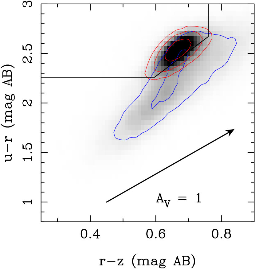
Figure 1.— The $u-r$ versus $r-z$ relation for galaxies in the $0.04<z<0.08$ from our SDSS sample in grey scale. Contours show the density of galaxies with $<2.5EW(H\alpha)/\sigma(EW(H\alpha))$ (red) and without $<2.5EW(H\alpha)/\sigma(EW(H\alpha))$ (blue). The contours are at 100, 300, and 1000 galaxies per color bin. The black lines have been chosen to minimize the difference between the number of galaxies with $<2.5EW(H\alpha)/\sigma(EW(H\alpha))$ within the box and the number of galaxies without $<2.5EW(H\alpha)/\sigma(EW(H\alpha))$ outside the box. This ensures robust separation of star-forming, late-type galaxies and quiescent, early-type galaxies even when spectroscopic information is not available, for example at higher redshifts.

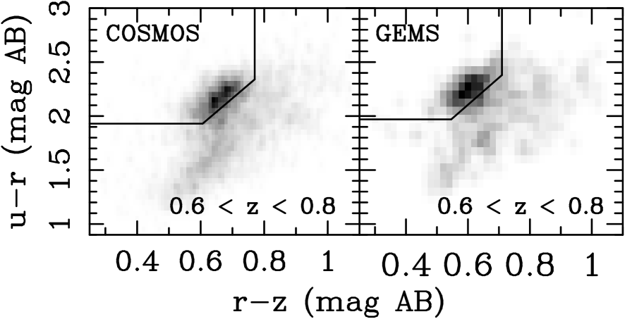
Figure 2.— The color-color relation for galaxies in the $0.6<z<0.8$ for COSMOS (left) and GEMS (right). The black lines show our color selection based on the lines from Fig. 1, shifted by the median colors of the quiescent population. As with Figure 1, the data have been lightly smoothed with a 1.5 pixel FWHM Gaussian before we plot the grey scales.

2.4. Stellar Mass Estimates

The DR7 catalog of Brinchmann et al. (2004) provides stellar mass estimates for the galaxies in our SDSS sample. These estimates use a new methodology for DR7, namely the spectral energy distributions are fit to the broad band photometry similar to the implementation of Salim et al. (2007) instead of using only the spectra as was done in the past. These differences are documented at http://www.mpa-garching.mpg.de/SDSS/DR7/. The model fit to the photometric data yields a distribution. We select the median mass value as the best estimate with the 16 and 84 percentile confidence limits as estimates of the errors.

In Figure 3 can be seen that quiescent galaxies obey a tight relation between color and stellar mass-to-light ratio – this is obviously inherent to the method. We derive a linear relation by computing the biweight mean in narrow color bins (0.02 mag wide) over the range $0.64<(g-r)_{0}<0.82$, where the sequence is well populated. A fit that minimizes the scatter in the biweight yields: $\log_{10}(M/L_{g})=-1.024+1.966(g-r)_{0}$. The scatter decreases from $\sigma=0.10$ to $\sigma=0.04$ in $\log_{10}(M/L_{g})$ over the probed color range.

For our high redshift samples, we would like to estimate stellar masses consistently. However, we cannot directly use the above relation because quiescent galaxies at $z\sim 0.7$ have had different star formation histories than their present-day counterparts, because, if nothing else, the universe was younger. We use independent constraints on the evolution of $(g-r)_{0}$ and $M/L_{g}$ to convert the above relation between color and $M/L$ for $z\sim 0.06$ galaxies to one appropriate for $z\sim 0.7$ galaxies. We take the evolution in $M/L_{g}$ from the recently derived fundamental plane evolution by Holden et al. (2010): $d\log_{10}M/L_{g}=(-0.60\pm 0.04)z$. We infer the $(g-r)_{0}$ color evolution by computing the biweight mean of the photometrically selected SDSS, GEMS, and COSMOS samples, for which find, respectively, $(g-r)_{0}=0.75$, 0.61, and 0.60. Thus, we shift the relation between $(g-r)_{0}$ and $M/L_{g}$ shown in Figure 3 to the left by 0.14 (COSMOS) or 0.15 (GEMS) mag, and down by 0.38 dex, resulting in stellar mass estimates that are $\sim 0.1$ dex lower at $z\sim 0.7$ than those for $z\sim 0.06$ at the same $(g-r)_{0}$ color.

To estimate errors on the stellar masses for the high redshift samples, we use the scatter in the $M/L_{g}$ versus $g-r$ relation at a the color of a given galaxy. This scatter is done in the relation after it is shifted by the mean $g-r$ color and $M/L$ evolution. We then add in quadrature the uncertainties in the zero point of the $M/L$ evolution. Thus the error in the high redshift stellar masses range from 0.06 to 0.11 dex depending on the color of the galaxy.

If use the $M/L$ evolution from the field sample of van der Wel et al. (2005), we would estimate smaller masses at $z=0.7$ by 0.02 dex, a small systematic shift. This difference is in good agreement with the statistical errors of the van der Wel et al. (2005) and Holden et al. (2010) samples.

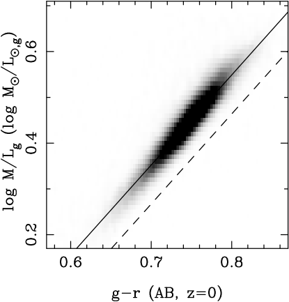
Figure 3.— The $g-r$-$M/L_{g}$ relation for early-type galaxies in SDSS ($M>1.25\times 10^{10}\ M_{\sun}$; $0.04<z<0.08$) selected by their $u-r$ and $r-z$ colors (see Figure 1). The solid line is the best-fitting relation. To estimate masses for our $z\sim 0.7$ masses from COSMOS and GEMS in a consistent manner we use the dashed line which has the same slope but a different zero point to compensate for evolution in the color and the mass-to-light ratio as explained in the text.

2.5. Projected Axis-Ratio Measurements

Our projected axis-ratio measurements, $q_{proj}$, come from two approaches. For the GEMS and COSMOS samples, these values are the result of fitting Sérsic models (Sérsic, 1968) to the two-dimensional images using the software GALFIT (Peng et al., 2002). For the SDSS catalog, we use the estimates from fitting a de Vaucouleurs model as part of the SDSS DR7 photometric pipeline (Abazajian et al., 2009).

The GEMS fits are contained in the catalog of Häussler et al. (2007). These are done using GALFIT as part of larger package known as GALAPAGOS. GALAPAGOS has the advantage of automating the catalog construction and model fitting process. The software automatically fits neighboring objects and incorporates its own sky subtraction algorithm in order to ensure robust parameter measurements. A more thorough discussion can be found in Häussler et al. (2007).

Griffith & Stern (2010) used GALAPAGOS to produce publicly available catalogs for both COSMOS and GEMS. We will use the catalog of Griffith & Stern (2010) for COSMOS and the catalog of Häussler et al. (2007) for GEMS, though,as we show below, there is no measurable difference between the Griffith & Stern (2010) and the Häussler et al. (2007) catalogs.

2.5.1 Consistency and Reliability of Projected Axis-Ratio Measurements

Our analysis hinges on the consistent measurement of the axis-ratios of galaxies at very different redshifts and from very different imaging data sets. In Holden et al. (2009), we tested our our axis-ratio measurements from GALFIT with simulations of observations of high redshift galaxies using real low redshift galaxies as templates. We found these measurements to be robust, with a negligible shift in the axis-ratio from $z=0$ to $z=1$ of $\delta q_{proj}\simeq-0.01$ with a scatter of $\sigma_{q}\simeq 0.01-0.03$ depending on galaxy magnitude.

In addition to data-related differences, the fitting algorithms also differ between the low- and high-redshift galaxy samples. We use the adaption of GALAPAGOS for SDSS imaging from Guo et al. (2009) to measure the axis-ratios of a sub-sample of our SDSS galaxies in a manner that is fully consistent with the treatment of the high-redshift galaxies. For small axis-ratios, systematic differences are expected to be largest. Therefore, we select 412 SDSS galaxies from our sample with axis-ratios $0.3<q_{proj}<0.305$ as determined by the SDSS pipeline. These represent the extreme end of the distribution, where systematic differences in fitting procedures or the point spread function should be the most manifest. The axis-ratio measurements from GALAPAGOS are fully consistent with the SDSS pipeline measurements: $\delta q_{proj}=q_{GALAPAGOS}-q_{SDSS}=0.01\pm 0.03$, where 0.03 is the root mean-squared scatter.

GALAPAGOS includes many free parameters that affect source detection, sky subtraction and treatment of neighbors. However, regardless of the different set ups that Häussler et al. (2007) and Griffith & Stern (2010) used for the GEMS data set, there is no systematic difference between the two catalogs for the objects in our sample ($\delta q_{proj}=0.02\pm 0.03$).

A final test of the robustness of our measurements is a comparison between axis-ratio measurements from those galaxies in the GEMS that lie within the much deeper ACS images from GOODS (Giavalisco et al., 2004). The difference is $\delta q_{proj}=-0.01$ with a scatter of $\sigma_{q}=0.05$. The negligible systematic difference is encouraging.

Summarizing, all tests and simulations stress that our axis-ratio measurements across the different data sets at different redshifts and performed with different algorithms, are internally fully consistent.

2.6. Completeness

We would like to measure evolution of the axis-ratio as a function of stellar mass. In order to probe as far down the mass function as possible, we need to limit our sample to above the mass limit where the initial survey photometry is complete.

For the SDSS, we find that our sample will have no bias as a function of redshift for early-type galaxies with a mass of $3\times 10^{10}\ M_{\sun}$ for the whole redshift range of $0.04<z<0.08$. This means that galaxies above that mass range have an equal probability of being included regardless of redshift. For the mass of $1.25\times 10^{10}\ M_{\sun}$, this is correct for only the redshift range of $0.04<z<0.06$. For the rest of this paper, we will include the whole sample to first mass limit, $3\times 10^{10}\ M_{\sun}$. For the mass range $1.25\times 10^{10}\ M_{\sun}<M<3\times 10^{10}\ M_{\sun}$ we limit the redshift range to $0.04<z<0.06$.

At higher redshifts, we have two different samples with two different selections. The GEMS sample was selected using a $R$ limiting magnitude. In contrast, the catalog from COSMOS we use was based on a combination of $I$ and 3.6 $\mu$m imaging. Combining the completeness computations from Ilbert et al. (2010) with the 3.6 $\mu$m magnitude distribution of galaxies with masses $10^{10}<M/M_{\sun}<1.5\times 10^{10}$, we infer that our sample is complete in this mass range. We adopt $1.25\times 10^{10}\ M_{\sun}$ as our mass limit. From a similar estimate for the GEMS sample we infer a completeness limit of $3\times 10^{10}\ M_{\sun}$. For the rest of this paper, when we compare samples with masses $>3\times 10^{10}\ M_{\sun}$, we will be comparing the whole SDSS sample with the combined GEMS and COSMOS sample. For masses below that limit, we are only comparing a subset of the SDSS sample with $0.04<z<0.06$ with the COSMOS sample.

2.7. Axis-Ratio Dependence of the Observations

In star-forming disk galaxies, dust is often concentrated in the mid-plane. This causes a strong color-dependence in the axis-ratio. For example, Maller et al. (2009) finds a slope of $\sim$-0.5 in the $u-r$ color with $q_{proj}$.

For our sample of early-type SDSS galaxies, we find that the slopes of the $u-r$ axis-ratio relation are small, -0.07 to -0.09 magnitudes, depending on galaxy mass. Thus, rounder galaxies are mildly bluer than thinner galaxies. These shallow slopes for our early-type population has two implications. First, the completeness our sample is not drastically impacted by the apparent axis-ratio of the galaxy. Second, that our sample of early-type galaxies are optically thin. This second criteria implies that the selection in color-color space removes galaxies with significant amounts of gas and dust, which is typical for passively-evolving systems.

Though the slopes of the $u-r$ color with axis-ratio are small in our SDSS DR7 sample, they still could be the result of our color-color selection. Therefore, we measured the relation of the $u-r$ color with axis-ratio for the sample of galaxies with $<2.5EW(H\alpha)/\sigma(EW(H\alpha))$ for comparison. We found statistically indistinguishable slopes in the $u-r$ versus $q_{proj}$ relation.

3. Intrinsic Shapes of $0.04<z<0.08$ Early-Type Galaxies

We plot the axis-ratio distribution as a function of stellar mass for the 33086 galaxies in our final SDSS DR7 sample in Figure 4. In that figure, we also plot the axis-ratio distributions in three broad mass bins. There are two obvious features in Figure 4. At high stellar mass, there is a clear absence of elongated objects, implying the absence of high-mass, disk-dominated, passively-evolving galaxies at both $z=0.6-0.8$ and at $z\sim 0$, as was seen in vdW09. Second, below a threshold mass of $\sim 10^{11}\ M_{\sun}$, we find a much broader distribution of galaxy axis-ratios, implying a significant population of disk-dominated galaxies (van der Wel et al., 2010, vdW10).

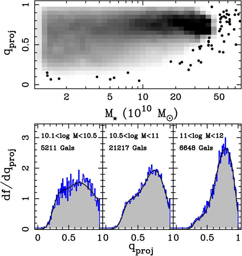
Figure 4.— The distribution of axis-ratios as a function of stellar mass for quiescent galaxies in the SDSS (top). When drawing the grey scale we normalize by the number of data points in each mass bin. Individual points represent galaxies where the number per bin would be less than three. The sample is complete to $3\times 10^{10}\ M_{\sun}$ for $0.04<z<0.08$, and to $1.25\times 10^{10}\ M_{\sun}$ for $0.04<z<0.06$. The narrowing of the distribution shows the threshold for early-type, disky galaxies, as seen by vdW09 and Bernardi et al. (2010). In the bottom panels, we plot the differential distribution of axis-ratios in three mass bins (marked by the vertical lines in the top panel with the log of the range in solar mass given). The number of early-type galaxies in each bin is given below the mass range. We over plot, in black, parametric models of the data described in Sec. 3.1.

3.1. A Parametric Description of the Data

We model the observed, projected axis-ratio distribution to infer the intrinsic axis-ratio distribution, assuming two types of toy models: triaxial systems and oblate spheroids. We use triaxial models because they are well motivated by other results which include galaxy kinematics (see, for example Franx et al., 1991; van den Bosch et al., 2008). We use the triaxial model of Franx et al. (1991) which has two components, a triaxiality, $T=\frac{a^{2}-b^{2}}{a^{2}-c^{2}}$, and an ellipticity $\epsilon=1-c/a$ where $a$, $b$, and $c$ are the three different axis making up the triaxial system, with $a$ being the largest and $c$ being the smallest. We assume that both of these quantities are distribution as Gaussian and so fit $\bar{T}$, $\bar{\epsilon}$, along with $\sigma_{T}$ and $\sigma_{\epsilon}$.

Our second model is a subset of the triaxial model, namely the oblate spheroid model is defined by fewer parameters. We use the formalism of Sandage et al. (1970) to describe the oblate spheroid component of the distribution. The free values are the minimum apparent axis ratio, $b$, corresponding to thickness of the spheroid. Once again, we assume a Gaussian distribution around $\bar{b}$ of size $\sigma_{b}$. The oblate spheroid model can be reproduced by a triaxial model with $T=0$ and $\sigma_{T}=0$.

3.1.1 The Fitting Process

We fit a number of models to the data simultaneously, ranging from one to three. If we fit more than one, we add additional fractions, $f$ which is simply the fraction of overall model distribution that is represented by a given component. To determine the best fitting model, we maximize the log likelihood assuming a Poisson distribution. Because the triaxial models are computationally intensive, we pre-compute the apparent axis-ratio distribution for a grid of values of $T$ and $\epsilon$. To compare our data with models, we must then bin the data to same binning as our precomputed triaxial models, or bins of $\delta q_{proj}=0.01$. For a given set of model parameters $M=M(\bar{T_{1}},\sigma_{T},1,\bar{\epsilon_{1}},\sigma_{\epsilon,1},\bar{T_{2}},....)$, we compute the relative probability for each bin in $q_{proj}$. We adjust the normalization such that the model has the same number of galaxies as the input sample, and can now compute the Poisson log likelihood $\log L_{i}=n_{i}\log(m_{i})-m_{i}-\log(n_{i}!)$ for each bin $i$ where $n_{i}$ is the number of galaxies in that bin and $m_{i}$ is the number predicted by the model with parameters $M$. We use a Monte Carlo Markov Chain to fit the distribution of axis-ratio values.

3.1.2 Fitting the $z\sim 0.06$ Galaxy Sample

We begin the fitting process with a single model, namely a triaxial distribution. In general, when fitting triaxial models to only the axis-ratio distribution, the triaxiality is not well constrained. This is a simple consequence of the fact the data are a single, projected value while our model contains two different axes. For galaxies with $M<10^{11}\ M_{\sun}$, we find that a single component is not an adequate description of the data, with the model producing a deficit of galaxies at larger $q_{proj}$ values and an overabundance of galaxies at small $q_{proj}$’s. Above that mass threshold, a single triaxial model appears to match the data well, however.

The addition of a second, oblate spheroid model matches the data much more closely. We plot these model fits, along with the SDSS data in blue, in Figure 4. Comparing the log likelihood values of the single model and two component model shows that the two component model is a better description of the data at a statistically significant level ($>3\sigma$).

Finally, we add a third triaxial component. In general, whether we fit three independent triaxial components or an oblate disk with two independent triaxial components, the fitting process de-weights the third component. The resulting model is dominated by only two components, which make up $>$90% of the model. For the rest of the paper, we will use the two component model with one constrained to be an oblate spheroid for simplicity.

3.2. Model Results for $z\sim 0.06$

For the highest mass bin, we find a low oblate spheroid fraction, 13 $\pm$ 4 %. The best fitting model has $T\simeq 0.4$, near a triaxial model in the formalism of Franx et al. (1991). This is close to the results found in that paper, and what we expected for large, dispersion supported systems.

Below $10^{11}\ M_{\sun}$, we can see the long, flat distribution to small axis-ratios well described by an oblate spheroid. In the middle mass bin, the fraction of oblate spheroids is 54 $\pm$ 6% and it grows to 70 $\pm$ 8% in the lowest mass bin. Interestingly, for the middle mass bin, the triaxial component has a very similar shape distribution as the triaxial component at higher masses.

One of the more robust parameters for even the triaxial models are the minor to major axis-ratios. In Figure 5, we plot the inferred distribution from the Monte Carlo Markov Chain of $c$, or the minor to major axis-ratios. The two different components to our model are readily apparent, along with their relative weight.

Most striking, in even the high mass bin, there are no really round galaxies. The modal value for $c$ is inferred to be $c\simeq 0.65$ or a ratio of $1.5$ to 1. Such an apparently small minor axis-ratio is actually in good agreement with the data. The intermediate axis, assuming a $T=0.4$ or so, will be $b=0.9$ and so such systems will often appear to close to but not perfectly round, exactly as we see in Figure 4.

The second result is that, in all mass bins, there are no very thin galaxies. Among the star-forming galaxy population, disks can can thin $c\simeq 0.2$ , especially at lower masses and even in red pass-bands (Ryden, 2006; Padilla & Strauss, 2008). Our modal value for the lowest mass bin in Figure 5 is 0.25 and the median value for the whole of the distribution is 0.29. Thus, the low-mass, passively evolving population is $\sim$50% thicker than similar mass active star-forming galaxies which have values more like $0.2$.

Figure 5.— The intrinsic axis-ratio distribution ($dn/dc$), where $c$ denotes the smallest-to-largest axis-ratio, in three mass bins for early-type galaxies in the SDSS. These plots represent our inferred results weighted by the likelihood distribution combined with our Gaussian model parameters. The model used to infer these distributions consist of an oblate component (where $c=b$) and a triaxial component (where $c=1-\epsilon$) – see Sec. 3.1 for a detailed description of this model and how the results are represented here. While details depend on the modeling assumptions, high-mass early-type galaxies typically have intrinsic short-to-long axis-ratios of 2:3, while $M^{\star}$ early-type galaxies typically have 1:3.

4. Shape Evolution of Early-type Galaxies

The final $0.6<z<0.8$ samples contain 1332 galaxies in total (171 from GEMS; 1161 from COSMOS) with masses greater than $1.25\times 10^{10}\ M_{\sun}$, though see Sec. 2.6 for details on the completeness with mass. We will now use these samples to measure the evolution of the axis-ratio distributions for samples in a fixed mass range.

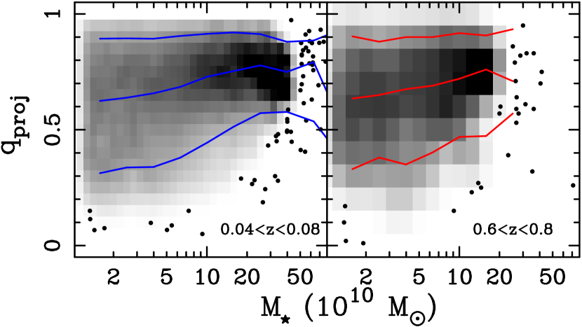
Figure 6.— The distribution of axis-ratios as a function of stellar mass for quiescent galaxies for the SDSS (left) and our combined COSMOS and GEMS $0.6<z<0.8$ sample (right). The SDSS data are the same as shown in Figure 4. In each, we over-plot the 10th percentile, median and 90th percentile axis-ratios as a function of mass for both the SDSS (blue) and the $0.6<z<0.8$ sample (red). At masses of $>3\times 10^{10}\ M_{\sun}$, the patterns appear indistinguishable in the two samples, with a steady tapering above $2\times 10^{11}\ M_{\sun}$ yielding an effective ceiling mass for high elongated system. This implies that the threshold for early-type, disky galaxies seen at low redshift by vdW09 and Bernardi et al. (2010) does not significantly evolve out $z\simeq 0.7$. Correspondingly, below that ceiling mass, both samples show similar distributions. This implies that at $z\sim 0.7$ the $M^{\star}$ early-type galaxy is moderately “disky”, as we show in Figure 5. In contrast, the mass density of early-type galaxies grows between $z\simeq 0.7$ and $z=0$. Our result shows that the mass growth must roughly preserve the distribution of axis-ratios in each mass bin.

4.1. The Shape Distribution of $0.6<z<0.8$ Galaxies

The combined sample of GEMS and COSMOS, along with the corresponding SDSS sample, can be seen in Figure 6. We plot the axis-ratio distribution as a function of stellar mass for the $0.04<z<0.08$ and $0.6<z<0.8$ samples. In Figure 7, we plot axis-ratio distribution in three broad mass bins, showing both the differential and cumulative distributions. There are two obvious features in Figure 6. At high stellar mass, there is a clear absence of elongated objects, implying the absence of high-mass, disk-dominated, passively-evolving galaxies at both $z\sim 0.7$ and at $z\sim 0$, as was seen in vdW09. Second, below a threshold mass of $\sim 10^{11}\ M_{\sun}$, we find a much broader distribution of galaxy axis-ratios, implying a significant population of disk-dominated galaxies (van der Wel et al., 2010, vdW10).

We use the parametric models we discuss in Sec. 3.1 to fit the distribution of data in Fig. 7. Because of the much smaller sample size, we fit the data with both the same models as we did the SDSS but also freeze some subsets of the parameters. In every case, we find that, within the limits of the uncertainties from the fits, the data can be described by the same model at both redshifts.

The clear similarity between the axis-ratio distributions of our low- and high-redshift samples shows that a ceiling mass for quiescent, disk-dominated galaxies exists at least since $z\sim 1$, generalizing the low-redshift result from vdW09. It is clear that, above $10^{11}\ M_{\sun}$, we find few flat galaxies. In contrast, these galaxies make up a much larger proportion of the population at masses below $10^{11}\ M_{\sun}$. Therefore, at $z\sim 0.7$, there is the same threshold for the population of “disky” early-type galaxies, that is found at $z\sim 0$.

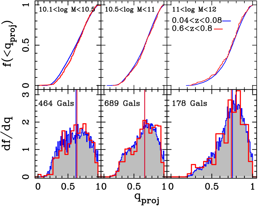
Figure 7.— The axis-ratio distribution for our early-type galaxy samples in three mass bins, with top and bottom showing the normalized cumulative and differential distributions respectively. The SDSS data are plotted with a blue line, in both, and grey shading in the bottom panels, while, we show our combined sample of early-type galaxies at $0.6<z<0.8$ in red. The total number of galaxies in the $0.6<z<0.8$ sample is given in the bottom panels, with the size of the SDSS samples for the same mass range given in Figure 4. We plot the median axis-ratio for the SDSS with a blue vertical line and the $0.6<z<0.8$ sample as a red line. The axis-ratio distribution is statistically similar in all three mass bins, with only the lowest mass bin showing a hint of evolution. Because statistically similar models as in Fig. 5 describe the $0.6<z0.8$ sample, out to z$\sim$1, massive early-types have axis-ratios of 2:3 while early-types around $M^{\star}$ show a thinner distribution closer to 1:3.

4.2. The Axis-Ratio Dependence of the Mass Function of Early-type Galaxies

Previous work has found a significant amount of evolution in the mass function of early-type galaxies (Wolf et al., 2003; Bell et al., 2004; Borch et al., 2006; Brown et al., 2007; Faber et al., 2007; Cirasuolo et al., 2007; Ilbert et al., 2010; Brammer et al., 2011). Generally, the evolution appears at the lower mass end. As we have found that the axis-ratio distribution also changes with mass, with more disk-like early-types at lower masses, we will investigate if the mass function evolution is different for different sub-populations as selected by axis-ratio.

We fit the mass distribution using a Schechter function. We use a standard maximum likelihood approach assuming a Poisson likelihood model and perform the fits over the mass range where our sample is volume complete. Each galaxy has its own error estimate for the mass measurement, so we convolve the Schechter function individually to compute the likelihood distribution. Including the errors in the fitting process has the advantage of not causing $M^{\star}$ being forced to higher values because of the occasional statistical fluctuation in a mass measurement.

4.2.1 Edge on systems with $q_{proj}<0.4$

We select all galaxies with $q_{proj}<0.4$ and masses $>3\times 10^{10}\ M_{\sun}$. This selects disk-dominated systems that are viewed close to edge-on but above the mass limit where we are complete for the whole volume of both samples. We fit the mass distribution with a Schechter function with a fixed value of $\alpha=-0.7$ (Bell et al., 2003) for both our $0.6<z<0.8$ and SDSS sample. We find the value of $\log_{10}M^{\star}/M_{\odot}=10.68\pm 0.10$ (errors come from bootstrapping the data) for quiescent galaxies with $q_{proj}<0.4$. This value lies within $1\sigma$ of our $0.04<z<0.08$ field sample of $\log_{10}M^{\star}/M_{\odot}=10.58\pm 0.01$. We confirm the lack of strong evolution by using Monte-Carlo simulations where we adjust the mass distribution of the $z\simeq 0.06$ sample and create sub-samples of the same size as our high-redshift sample with the same mass limits. From this we find that the typical mass of $q_{proj}<0.4$ galaxies above our mass completeness limit can only shift by by $\pm 0.06$ dex, $\sim$16%, in our $0.6<z<0.8$ sample. We also confirm this result using non-parametric tests, the Kolmogorov-Smirnov test and the Mann-Whitney test, which also show no significant difference in the two samples.

4.2.2 Round systems with $q_{proj}>0.6$

We also look for evolution in the apparently round galaxy population, those with $q_{proj}>0.6$. From our modeling results in Sec. 3.1, we expect that this population is a combination of those mostly triaxial systems, with intrinsic ratios of 2:3, and the more flattened, or 1:3, population that dominates at lower masses. Evolution in this population, if not mirrored in the $q_{proj}<0.4$ population, would imply evolution in the more triaxial component of the population that dominates at high masses.

When we examine the galaxies that are round, $q_{proj}>0.6$, we find significant ($>3\sigma$) though mild amount evolution in the mass function. For our SDSS sample, we find $\log_{10}M^{\star}/M_{\odot}=10.93\pm 0.01$ while in our $0.6<z<0.8$ sample we find $\log_{10}M^{\star}/M_{\odot}=10.85\pm 0.02$. As before, we confirm this result at the $>3\sigma$ with the Kolmogorov-Smirnov test and the Mann-Whitney test. We also confirm this result by drawing sub-samples of galaxies from the $q_{proj}>0.6$ and $0.04<z<0.08$ SDSS sample of the same size as the $0.6<z<0.8$ sample. We find that these sub-samples recover $\log_{10}M^{\star}/M_{\odot}=10.93$ with a scatter of $\pm 0.02$ dex. The larger question is, does this evolution represent a change in the galaxy population or is it a result of our measurements? Our $0.6<z<0.8$ stellar masses have a systematic uncertainty of $\pm 0.04$ dex. 2Thus, the shift in the mass function we find is interesting but not statistically significant. Because this an error on the zero point of stellar masses, which we derive from evolution in the fundamental plane (see Sec. 2.4), the systematic error on the stellar masses can be lowered in future work. This will confirm or refute this apparent evolution shape of the mass function of round early-type galaxies.

4.2.3 The whole of the population

As check on our mass functions, we fit for $M^{\star}$ with a fixed $\alpha=-0.7$ for whole of our $0.04<z<0.08$ sample of passively evolving galaxies and find $\log_{10}M^{\star}/M_{\sun}=10.87\pm 0.01\ M_{\sun}$, in good agreement with Bell et al. (2003) after accounting for differences in the IMF and $h$. We find $\log_{10}M^{\star}/M_{\sun}=10.85\pm 0.02\ M_{\sun}$ for our high redshift sample, similar to Borch et al. (2006). In Figure 8, we show the mass functions for three selections in axis-ratio ($q_{proj}<0.4$, $q_{proj}>0.6$ and all galaxies regardless of $q_{proj}$). We also plot our estimate of the total number density of galaxies per logarithmic density bin. It is clear that we recover the trend in the density evolution of the passive galaxy population found by Ilbert et al. (2010). We note that Ilbert et al. (2010) found evolution in $\alpha$. We find that, because of our high mass limit of $3\times 10^{10}\ M_{\sun}$, we have little statistical constraint on the best fitting value of $\alpha$. To improve our results would require implementing completeness corrections for both samples. Nonetheless, we reproduce $M^{\star}$ with the same sample. Thus, despite our different methodology for determining stellar masses and different sample definitions, we find consistent results with other measurements of the mass function.

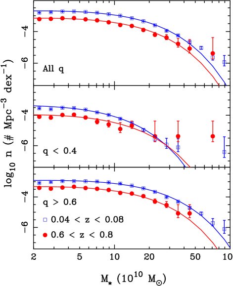
Figure 8.— Mass functions of the $0.04<z<0.08$ (red filled circles) and $0.6<z<0.8$ (blue open squares) samples, for three different axis-ratio ($q_{proj}$ )selections. We over plot with solid lines the best fitting Schechter functions, all assuming a fixed $\alpha=-0.7$. Our fitting process includes the errors on the stellar mass estimates. Reinforcing the visual impression from Figure 6, the mass function of flat galaxies has a much smaller value of $M^{\star}$ than the mass function of almost round galaxies. There is also little evolution in the shape of the mass function except for possibly the $q_{proj}>0.6$ sample, see text for further discussion. In general, the volume density of galaxies evolves by a factor of $\sim\times$2-3 at $10^{11}\ M_{\sun}$, in good agreement with the evolution seen in Bundy et al. (2010) or Ilbert et al. (2010). This evolution is the same, regardless of the axis-ratio of the population. This requires that the growth in the mass density of galaxies, in the mass range we consider, must occur in a manner that preserves the overall shape distribution.

4.3. The Bulge-to-Disk Ratio of the Population of Early-type Galaxies

The average axis-ratio of a galaxy population is directly determined by the populations average bulge-to-disk ratio (Binney & Merrifield, 1998), assuming that bulges are drawn from a different axis-ratio distribution as compared with disks (see Figure 2 of Dutton et al., 2011, which shows that this is true for all but the highest mass galaxies). Therefore, by examining the evolution of the axis-ratio of the population, we are determining whether or not the population becomes more bulge-dominated or disk-dominated as a function of time, though we cannot determine if this evolution happens for individual galaxies or because of a changing mix of bulge-to-disk ratios in the population.

In the range $3\times 10^{10}\ M_{\sun}<M<10^{11}\ M_{\sun}$, we find no difference in axis-ratio distribution between the two redshift slices. In the lowest-mass bin ($1.25\times 10^{10}\ M_{\sun}<M<3\times 10^{10}\ M_{\sun}$) we see a small but barely significant difference between the two samples, suggestive of a more disk-dominated population in the $0.04<z<0.08$ sample. Because of the low significance of the difference ($2.4\sigma$) and the fact that it occurs in the smallest mass bin where the completeness is lowest, we consider this difference an interesting but tentative result.

5. Discussion and Conclusions

5.1. A Universal Ceiling Mass for Flattened Early-type Galaxies

vdW09 observed a ceiling mass of $\sim 10^{11}\ M_{\sun}$ for disk-dominated, quiescent galaxies in the present-day universe. In accordance, Bernardi et al. (2010) found that early-type galaxies with very high masses ($\sim 2\times 10^{11}\ M_{\sun}$) differ in many ways from those with lower masses ($<10^{11}\ M_{\sun}$). In this paper we show that a similar transition mass exists at $z\sim 0.7$ and that its value has not shifted by more than 0.05 dex between $z\sim 0.7$ and the present. Thus, at all redshifts, roughly 40% of the stellar mass in early-type systems is contained in these relatively round systems. As expected from Figure 4, round systems ($q_{proj}>0.6$) have a characteristic mass of $M^{\star}\sim 9\times 10^{10}\ M_{\sun}$ while highly flattened ($q_{proj}<0.4$), passively evolving galaxies have $M^{\star}\sim 4\times 10^{10}\ M_{\sun}$. We find no significant evolution in the value for $M^{\star}$ between our two samples, only evolution in the co-moving number density.

This mass ceiling has the same mass, or, in other words, $M^{\star}$ does not evolve for more elongated or “disky” early-type galaxies despite the growth of the passively evolving population by a factor of $\sim 2-3$ in mass between $z\sim 1$ and today (see Figure 8; Wolf et al., 2003; Bell et al., 2004; Borch et al., 2006; Brown et al., 2007; Faber et al., 2007; Cirasuolo et al., 2007; Ilbert et al., 2010; Brammer et al., 2011). This has two implications. First, the progenitors of today’s population of massive early-type population were not more disk-dominated systems at $z=0.7$ that faded into the passively-evolving population. Instead, these galaxies must already be almost round, roughly 2:3 in intrinsic axis-ratio, galaxies before the truncation of star-formation (see Kocevski et al., 2010, for candidate progenitors). Second, if merging builds up the population of galaxies above $\sim 10^{11}\ M_{\sun}$, that merging most cause them to become rounder systems.

5.2. Implications for the Formation of Galaxies with $M>10^{11}\ M_{\sun}$

At the highest masses, we find that, not only is there a lack of flattened or “disky” galaxies, but that the distribution is consistent with a largely triaxial population. This can be seen by the lack of galaxies that are round in projection galaxies at high masses in Figure 4. These apparently round galaxies are seen at lower masses, so we do know that the lower fraction of high mass, round galaxies not just a systematic measurement error. Padilla & Strauss (2008) found a similar result, but the lack of evolution we find means that this triaxiality is set in the formation of these systems out to $z\sim 1$. This result, when combined with the observed evolution in the normalization of the mass function, and hints about the shape (see 4.2.2), this triaxial population is built up over the redshift range we observe, but is done so in such a way to produce similar shaped systems over that time.

Massive ellipticals are assumed to form out of multiple mergers of near equal mass systems and the merger rate is expected to be high even at redshifts of $z\sim 0.7$ (e.g. De Lucia & Blaizot, 2007). Detailed simulations with cosmological initial conditions show that additional mechanisms are required to reproduce the observed shapes and kinematic profiles of massive ellipticals (e.g. Burkert et al., 2008; Novak, 2008). Minor mergers and tidal encounters also provide a mechanism for making the most massive quiescent galaxies appear round. Vulcani et al. (2011) finds that the most massive cluster galaxies, objects too massive to be in our sample, are less round at high redshift. This points to observational evidence of the process of galaxies becoming rounder with time, possibly because of the mechanisms suggested in Burkert et al. (2008), but only for the rarest and most extreme of systems.

5.3. Evolution of the $\sim M^{\star}$ Early-type Population

At masses $<10^{11}\ M_{\sun}$, the early-type population becomes more and more “disky”. This can be seen in two ways, first, we find more round galaxies, $q_{proj}>0.9$. Second, we find more flattened systems, $q_{proj}<0.4$. This can be seen in both the minimum axis-ratio we find in Figure 4, and, the distribution of $c/a$ values we infer from our parametric modeling in Figure 5.

Quiescent galaxies with masses that dominate the cosmic stellar mass budget ($3\times 10^{10}\ M_{\sun}<M_{\star}<10^{11}\ M_{\sun}$) show a broad but non-evolving range in axis-ratios, at both $z\sim 0.7$ and $z\sim 0.06$. The broad range in axis-ratios implies that the population can form through a number of channels. Because we find so little evolution in the axis-ratios, however, means that, whatever the mechanisms that form early-type galaxies in this mass range, they must have worked at similar rates across the last 7-8 Gyrs of look-back time. This evolution cannot explained entirely by the increase in the number of bulge-dominated galaxies (say, merger products), nor can it be explained entirely by the cessation of star formation in disk-dominated galaxies without structural changes. Several evolutionary processes that cause the formation of quiescent galaxies must contribute in order to explain the unchanging fractions of bulge- and disk-dominated quiescent galaxies. Moreover, the relative importance of the various evolutionary processes has not strongly changed over the past 7-8 Gyrs. This is reminiscent of the general result that the morphological mix of galaxies of these masses does not significantly change over the same time (vdW07, H09, Bundy et al., 2010).

5.3.1 Growth in the Number Density Growth of Highly Flattened Systems

Our work finds consistent evolution in the number density of passively evolving galaxies with redshift. Most work finds significant evolution, factors of 2 or 3, in the number density of galaxies in the mass range of our sample(e.g. Ilbert et al., 2010; Bundy et al., 2010; Brammer et al., 2011). The combination of a flattened population at low masses with the increased number density of galaxies with redshift says that, at lower masses, the buildup of the mass function of passively evolving galaxies, or early-types, is the build up of passive disk-like galaxies, such as S0s or “disky” ellipticals (Bundy et al., 2010).

How can we explain the existence and continued growth of a population of quiescent, flattened galaxies? Gas stripping in group and cluster environments has long been argued to play a role (Spitzer & Baade, 1951), and was recently shown to explain the existence of the morphology-density relation (van der Wel et al., 2010). Our tentative detection of an increased fraction of “disky”, quiescent low-mass galaxies ($<3\times 10^{10}\ M_{\sun}$) at late times may indicate that this process is becoming increasingly important at late cosmic epochs.

5.3.2 Structural Properties and Merging

It is clear that all disk-dominated, quiescent galaxies cannot be the result of gas stripping, especially those outside massive groups and clusters (e.g. Dressler, 1980). While this may be feasible in the form of efficient gas stripping from satellite galaxies, even in sparser group environments (van den Bosch et al., 2008), the observed differences between disky quiescent galaxies and star-forming spiral galaxies of the same mass imply that the former are not, generally, stripped versions of the latter. Quiescent galaxies typically have fewer bars (Aguerri et al., 2009; Laurikainen et al., 2009), larger bulges (Dressler, 1980; Christlein & Zabludoff, 2004; Ryden, 2006; Laurikainen et al., 2010) and are more concentrated (Bundy et al., 2010) than star-forming galaxies, though many of these properties are mass dependent (Cheng et al., 2011). Finally, the axis-ratio distributions of star-forming galaxies are markedly different, much flatter as expected for an oblate spheroid population alone, then the distributions we observe for early-type galaxies (Ryden, 2006; Padilla & Strauss, 2008) Thus, at least at higher masses, the truncation of star formation must be intimately linked with bulge growth (e.g. Bell, 2008), even if a sizable stellar disks remains intact.

Minor merging may provide a possible path, which would provide a natural explanation for our observation that the mix of bulge- and disk-dominated quiescent galaxies remains unchanged at $z\lesssim 1$. The advantage of this mechanism is that minor merging is common, it produces most of the growth for massive early-type galaxies (for example Oser et al., 2011). Second, the amount of minor mergers grow bulges (e.g. Kauffmann et al., 1993; Baugh et al., 1996), though that depends on the gas content of the smaller system (Mihos & Hernquist, 1994; Hopkins et al., 2009).

Because of this, Bundy et al. (2010) suggests a two stage scenario. First, some feedback mechanism causes star-formation to cease. Second, because lower gas content galaxies have more rapid bulge growth from minor mergers (Hopkins et al., 2009), the resulting remnants are both passively evolving and bulge-dominated. In fact, bulge growth through minor merging may cease star formation as a result of gas exhaustion, some feedback mechanism (possibly AGN), or the stabilization of a gaseous disk against star formation (e.g. Bower et al., 2006; Croton et al., 2006). The main problem with such a process is, however, that we find no evolution in the overall axis-ratio distribution. This means this two stage process must produce as many bulge-dominated systems as new disk-dominated systems are added to the early-type galaxy population. If the rate of these two processes are not in good agreement, we would see a change in the distribution with time, the opposite of what our data show. This argues that the bulge growth and disk truncation should go hand in hand. If merging is the dominate physical process, this would imply some component of the merging

A dynamical process is required to turn the average star-forming galaxy into the typical early-type galaxy, for the reasons we list above. This process must generate a larger bulge fraction and population with an axis-ratio distribution that is markedly different from the flat population seen for star-forming systems (Ryden, 2006; Padilla & Strauss, 2008, e.g.). The most likely mechanism is merging, as merging changes the axis-ratio of galaxies with low gas masses. Some combination of major merging and minor merging, with more emphasis on the later due to its larger frequency, is the most likely culprit for structurally transforming active star-forming galaxies into the passively evolving galaxies we observe both today and at $z\sim 1$.

5.4. Future Directions

Our study uses a simple measurement (the projected axis-ratio) to come to arrive at far-reaching conclusions about the evolution of galaxy structure. The caveat is that we rely on the assumption that flattened systems have significant rotational support. It also rests on the assumption that one number to characterize the intrinsic shape is a sensible approximation, allowing us to bypass bulge-disk decompositions (MacArthur et al., 2008; Laurikainen et al., 2010; Simard et al., 2011) and spatially resolved, stellar dynamics (van der Marel & van Dokkum, 2007a, b; Krajnovic et al., 2008; van der Wel & van der Marel, 2008), which are notoriously difficult at high redshift. So far, such studies support our conclusions, most explicitly by the observation that the fraction of rotationally supported early-type galaxies is similar at $z\sim 1$ and in the present-day universe (van der Wel & van der Marel, 2008).

An interesting question is whether the absence of a significant population of very massive disk-like galaxies at $z\lesssim 1$ is a fundamental feature of galaxy formation. Perhaps under circumstances that are met at much earlier epochs than $z\sim 1$ such galaxies can and do exist, and the observations presented in this paper merely show that merging, either minor or major, is the only relevant mechanism to produce very massive galaxies at relatively recent epochs. Observations of significantly large samples of very massive galaxies at $z\sim 2$ may provide answer and do show some hints (van der Wel et al., 2011). The structural properties of galaxies at the epoch during which the star formation rate was highest will tell us whether galaxies with stellar masses $M>2\times 10^{11}\ M_{\sun}$ are always bulge dominated.

5.5. Conclusions

In this paper we analyze the projected axis-ratio distributions of early-type galaxies with stellar masses $>1.25\times 10^{10}\ M_{\sun}$ at $z\sim 0.06$ and $z\sim 0.7$. By modeling the intrinsic distribution, we find that at least since $z\sim 1$, there is a stellar mass ceiling for flattened early-type galaxies. Above $10^{11}\ M_{\sun}$ such galaxies are increasingly rare, both at the present day and at $z\sim 0.7$ (see Figures 6, 7 and 8). This suggests that at all cosmic epochs the dominant evolutionary channel for early-type galaxies with higher masses is a dynamical process that transforms systems with a 1:3 intrinsic axis-ratio into a rounder, triaxial system with a roughly 2:3 axis-ratio.

Below that mass threshold, the early-type galaxy population becomes more and more dominated by flattened or disk-like systems, with roughly an axis-ratio of 1:3. This is manifest in the number of round galaxies as well as in the larger and larger number of galaxies that appear thin in projection. This geometric picture also fits very well with the kinematic evidence that shows that most such early types are ’rapid rotators’, at least in the present-day universe. Once again, the axis-ratio distribution appears to evolve little out to $z\sim 1$. The non-evolving shape of the mass function of flat versus round galaxies we find in Figure 8 coupled with the overall growth of the normalization implies that $M^{\star}$ early-type galaxies form in a similar way over the last 7 Gyrs. The growth mechanism must roughly double to triple the number of early-type galaxies, producing a mix bulge-to-disk ratios that varies with galaxy mass, but the process must not vary with time in the mass range we study. The leading puzzle for early-type formation is a unifying model for how to explain this growth in mass density with so little change in the shapes of galaxies over the same look-back time.

The authors would like to thank Erik Bell, Dan McIntosh, Greg Rudnick, Sandra Faber and David Koo for useful discussions, comments and feedback. BPH would also like to thank the scientists and staff of the Max Planck Institute for Astronomy in Heidelberg for hosting him while working on this project.

Facilities: HST (ACS) Sloan

References

- Abazajian et al. (2009) Abazajian, K. N., et al. 2009, ApJS, 182, 543
- Aguerri et al. (2009) Aguerri, J. A. L., Méndez-Abreu, J., & Corsini, E. M. 2009, A&A, 495, 491
- Baugh et al. (1996) Baugh, C. M., Cole, S., & Frenk, C. S. 1996, MNRAS, 283, 1361
- Bell (2008) Bell, E. F. 2008, ApJ, 682, 355
- Bell et al. (2003) Bell, E. F., McIntosh, D. H., Katz, N., & Weinberg, M. D. 2003, ApJS, 149, 289
- Bell et al. (2004) Bell, E. F., et al. 2004, ApJ, 608, 752
- Bernardi et al. (2010) Bernardi, M., Roche, N., Shankar, F., & Sheth, R. K. 2010, ArXiv e-prints
- Binney & Merrifield (1998) Binney, J., & Merrifield, M. 1998, Galactic astronomy (Galactic astronomy / James Binney and Michael Merrifield. Princeton, NJ : Princeton University Press, 1998. (Princeton series in astrophysics) QB857 .B522 1998 ($35.00))
- Blakeslee et al. (2006) Blakeslee, J. P., et al. 2006, ApJ, 644, 30
- Borch et al. (2006) Borch, A., et al. 2006, A&A, 453, 869
- Bower et al. (2006) Bower, R. G., Benson, A. J., Malbon, R., Helly, J. C., Frenk, C. S., Baugh, C. M., Cole, S., & Lacey, C. G. 2006, MNRAS, 370, 645
- Brammer et al. (2011) Brammer, G. B., et al. 2011, ApJ, submitted, arXiv1104.2595
- Brinchmann et al. (2004) Brinchmann, J., Charlot, S., White, S. D. M., Tremonti, C., Kauffmann, G., Heckman, T., & Brinkmann, J. 2004, MNRAS, 351, 1151
- Brown et al. (2007) Brown, M. J. I., Dey, A., Jannuzi, B. T., Brand, K., Benson, A. J., Brodwin, M., Croton, D. J., & Eisenhardt, P. R. 2007, ApJ, 654, 858
- Bruzual & Charlot (2003) Bruzual, G., & Charlot, S. 2003, MNRAS, 344, 1000
- Bundy et al. (2010) Bundy, K., et al. 2010, ApJ, 719, 1969
- Burkert et al. (2008) Burkert, A., Naab, T., Johansson, P. H., & Jesseit, R. 2008, ApJ, 685, 897
- Cardamone et al. (2010) Cardamone, C. N., et al. 2010, ApJS, 189, 270
- Chabrier (2003) Chabrier, G. 2003, PASP, 115, 763
- Cheng et al. (2011) Cheng, J. Y., Faber, S. M., Simard, L., Graves, G. J., Lopez, E. D., Yan, R., & Cooper, M. C. 2011, MNRAS, 412, 727
- Christlein & Zabludoff (2004) Christlein, D., & Zabludoff, A. I. 2004, ApJ, 616, 192
- Cirasuolo et al. (2007) Cirasuolo, M., et al. 2007, MNRAS, 380, 585
- Croton et al. (2006) Croton, D. J., et al. 2006, MNRAS, 365, 11
- De Lucia & Blaizot (2007) De Lucia, G., & Blaizot, J. 2007, MNRAS, 375, 2
- Dressler (1980) Dressler, A. 1980, ApJ, 236, 351
- Dutton et al. (2011) Dutton, A. A., et al. 2011, MNRAS, 1045
- Emsellem et al. (2011) Emsellem, E., et al. 2011, MNRAS, 414, 888
- Faber et al. (2007) Faber, S. M., et al. 2007, ApJ, 665, 265
- Franx et al. (1991) Franx, M., Illingworth, G., & de Zeeuw, T. 1991, ApJ, 383, 112
- Giavalisco et al. (2004) Giavalisco, M., et al. 2004, ApJ, 600, L93
- Griffith & Stern (2010) Griffith, R. L., & Stern, D. 2010, AJ, 140, 533
- Guo et al. (2009) Guo, Y., et al. 2009, MNRAS, 398, 1129
- Häussler et al. (2007) Häussler, B., et al. 2007, ApJS, 172, 615
- Holden et al. (2009) Holden, B. P., et al. 2009, ApJ, 693, 617
- Holden et al. (2007) —. 2007, ApJ, 707
- Holden et al. (2010) Holden, B. P., van der Wel, A., Kelson, D. D., Franx, M., & Illingworth, G. D. 2010, ApJ, in press
- Hopkins et al. (2009) Hopkins, P. F., Hernquist, L., Cox, T. J., Keres, D., & Wuyts, S. 2009, ApJ, 691, 1424
- Ilbert et al. (2010) Ilbert, O., et al. 2010, ApJ, 709, 644
- Ilbert et al. (2009) —. 2009, ArXiv e-prints
- Jørgensen & Franx (1994) Jørgensen, I., & Franx, M. 1994, ApJ, 433, 553
- Kauffmann et al. (1993) Kauffmann, G., White, S. D. M., & Guiderdoni, B. 1993, MNRAS, 264, 201
- Kocevski et al. (2010) Kocevski, D. D., et al. 2010, ApJ, submitted
- Kormendy & Djorgovski (1989) Kormendy, J., & Djorgovski, S. 1989, ARA&A, 27, 235
- Krajnovic et al. (2008) Krajnovic, D., et al. 2008, MNRAS, 807
- Laurikainen et al. (2009) Laurikainen, E., Salo, H., Buta, R., & Knapen, J. H. 2009, ApJ, 692, L34
- Laurikainen et al. (2010) Laurikainen, E., Salo, H., Buta, R., Knapen, J. H., & Comerón, S. 2010, MNRAS, 405, 1089
- MacArthur et al. (2008) MacArthur, L. A., Ellis, R. S., Treu, T., U, V., Bundy, K., & Moran, S. 2008, ApJ, 680, 70
- Maller et al. (2009) Maller, A. H., Berlind, A. A., Blanton, M. R., & Hogg, D. W. 2009, ApJ, 691, 394
- Marinoni et al. (1999) Marinoni, C., Monaco, P., Giuricin, G., & Costantini, B. 1999, ApJ, 521, 50
- Mihos & Hernquist (1994) Mihos, J. C., & Hernquist, L. 1994, ApJ, 437, L47
- Novak (2008) Novak, G. S. 2008, PhD thesis, University of California, Santa Cruz
- Oser et al. (2011) Oser, L., Naab, T., Ostriker, J. P., & Johansson, P. H. 2011, ApJ
- Padilla & Strauss (2008) Padilla, N. D., & Strauss, M. A. 2008, MNRAS, 388, 1321
- Patel et al. (2011) Patel, S. G., Holden, B. P., Kelson, D. D., Franx, M., van der Wel, A., & Illingworth, G. D. 2011, ApJ, submitted
- Patel et al. (2010) Patel, S. G., Holden, B. P., Kelson, D. D., Illingworth, G. D., & Franx, M. 2010, ApJ, in prep.
- Peng et al. (2002) Peng, C. Y., Ho, L. C., Impey, C. D., & Rix, H. 2002, AJ, 124, 266
- Rix et al. (2004) Rix, H., et al. 2004, ApJS, 152, 163
- Ryden (2006) Ryden, B. S. 2006, ApJ, 641, 773
- Salim et al. (2007) Salim, S., et al. 2007, ApJS, 173, 267
- Sandage et al. (1970) Sandage, A., Freeman, K. C., & Stokes, N. R. 1970, ApJ, 160, 831
- Scoville et al. (2007) Scoville, N., et al. 2007, ApJS, 172, 1
- Sérsic (1968) Sérsic, J. L. 1968, Atlas de Galaxíes de Australes (Cǿrdoba, Argentina: Observatorio Astronomico, 1968)
- Simard et al. (2011) Simard, L., Mendel, J. T., Patton, D. R., Ellison, S. L., & McConnachie, A. W. 2011, ApJS, in press
- Spitzer & Baade (1951) Spitzer, L. J., & Baade, W. 1951, ApJ, 113, 413
- van den Bosch et al. (2008) van den Bosch, F. C., Aquino, D., Yang, X., Mo, H. J., Pasquali, A., McIntosh, D. H., Weinmann, S. M., & Kang, X. 2008, MNRAS, 387, 79
- van der Marel & van Dokkum (2007a) van der Marel, R. P., & van Dokkum, P. G. 2007a, ApJ, 668, 738
- van der Marel & van Dokkum (2007b) —. 2007b, ApJ, 668, 756
- van der Wel et al. (2010) van der Wel, A., Bell, E. F., Holden, B. P., Skibba, R. A., & Rix, H. 2010, ApJ, 714, 1779
- van der Wel et al. (2005) van der Wel, A., Franx, M., van Dokkum, P. G., Rix, H.-W., Illingworth, G. D., & Rosati, P. 2005, ApJ, 631, 145
- van der Wel et al. (2009) van der Wel, A., Rix, H., Holden, B. P., Bell, E. F., & Robaina, A. R. 2009, ApJ, 706, L120
- van der Wel et al. (2011) van der Wel, A., et al. 2011, ApJ, 730, 38
- van der Wel & van der Marel (2008) van der Wel, A., & van der Marel, R. P. 2008, ApJ, 684, 260
- Vincent & Ryden (2005) Vincent, R. A., & Ryden, B. S. 2005, ApJ, 623, 137
- Vulcani et al. (2011) Vulcani, B., et al. 2011, MNRAS, 133
- Whitaker et al. (2010) Whitaker, K. E., et al. 2010, ApJ, 719, 1715
- Williams et al. (2009) Williams, R. J., Quadri, R. F., Franx, M., van Dokkum, P., & Labbé, I. 2009, ApJ, 691, 1879
- Wolf et al. (2009) Wolf, C., et al. 2009, MNRAS, 393, 1302
- Wolf et al. (2003) Wolf, C., Meisenheimer, K., Rix, H.-W., Borch, A., Dye, S., & Kleinheinrich, M. 2003, A&A, 401, 73
- Wuyts et al. (2007) Wuyts, S., et al. 2007, ApJ, 655, 51
- York et al. (2000) York, D. G., et al. 2000, AJ, 120, 1579