Impact of surface roughness on diffusion of confined fluids

Abstract

Using event-driven molecular dynamics simulations, we quantify how the self diffusivity of confined hard-sphere fluids depends on the nature of the confining boundaries. We explore systems with featureless confining boundaries that treat particle-boundary collisions in different ways and also various types of physically (i.e., geometrically) rough boundaries. We show that, for moderately dense fluids, the ratio of the self diffusivity of a rough wall system to that of an appropriate smooth-wall reference system is a linear function of the reciprocal wall separation, with the slope depending on the nature of the roughness. We also discuss some simple practical ways to use this information to predict confined hard-sphere fluid behavior in different rough-wall systems.

I Introduction

Predicting the dynamic properties of moderate-to-high density bulk fluids from first principles remains an outstanding scientific challenge. This already-difficult problem becomes considerably more formidable when the fluid is confined to small spaces, a situation that is commonly encountered across a broad range of technologically important settings.Bhushan et al. (1995) In recent years, an important step toward solving this problem for confined fluids was taken by identifying physically meaningful static (i.e., thermodynamic) variables (or combinations thereof) against which dynamic fluid properties scaled independently of the degree of confinement.Mittal et al. (2006, 2007a, 2007b, 2007c); Goel et al. (2008); Mittal et al. (2008); Goel et al. (2009); Mittal (2009) This identification suggested that dynamic properties such as the self diffusivity of confined fluids could be predicted based on knowledge of their static properties and the corresponding static-dynamics scaling relationship obtained from, e.g., bulk fluid data. To date, tests of this scaling strategy for predicting how confinement affects dynamics of model systems have been carried out by molecular simulation of monatomicMittal et al. (2006, 2007a, 2007b, 2007c); Goel et al. (2009); Mittal (2009) and a limited number of molecular Chopra et al. (2010) fluids. Although these tests suggest that the scaling method can successfully predict the dynamic behavior of a variety of fluids confined to pores with different geometries, little attention has been paid to the nature of the confining walls themselves and how it affects the relationship between static variables and dynamic properties. In this paper, we address this issue by investigating how surface roughness impacts the self diffusivity of model confined fluids.

Smooth, flat structureless walls represent a mathematically convenient and idealized theoretical construct, and thus, historically, have been commonly used in the study of model confined fluids. However, real solid surfaces do in fact exhibit structure, which can significantly impact the thermodynamic and dynamic properties of the fluids they contact. Wetting and lubrication are two obvious examples of phenomena where the structure and shape of the fluid-exposed solid surface have significant implications.Grzelak et al. (2010); Grzelak and Errington (2010) This should not be surprising because surface roughness, which arises from the structural arrangement of “wall” particles, ultimately influences the fluid-wall interaction. Also, it is clear that surface roughness greatly impacts dynamics. For low density gases, where Knudsen diffusionKnudsen (1909) dominates, self diffusion decreases with surface roughness.Arya et al. (2003); Malek and Coppens (2001, 2002, 2003) Furthermore, experiments of confined colloids find that some particles stick to walls, further slowing dynamics.Edmond et al. (2010) Simulations have shown that position-dependent relaxation processes near rough surfaces are much slower than those near smooth surfaces.Scheidler et al. (2002, 2004)

A question which has recieved comparatively less attention is how surface roughness impact the self-diffusivity of moderate-to-dense confined fluids. The goal of this paper is to answer this question systematically via molecular simulations. The most obvious way in which roughness influences dynamic properties is through the modification of fluid particle–wall collisions. Here, we investigate how different representations of this collisional modification lead to changes in the self-diffusion of a simple, confined fluid. As a starting point, we study the monodisperse hard-sphere (HS) fluid confined between smooth hard walls. Despite its simplicity, we choose the HS fluid because it captures many of the important effects arising from the dominant excluded volume interactions in liquids Errington et al. (2003); Hansen and McDonald (2006) Obviously, a smooth hard wall does not possess any roughness whatsoever, but it still serves as a useful reference point for studying confined fluids, specifically the dynamic properties in this paper. In fact, the slit pore geometry is often assumed when determining the pore size distribution from adsorption isotherms in real porous materials.Lastoskie et al. (1993); Olivier et al. (1994); Lastoskie et al. (1997); Rouquerol and Rouquerol (1999); Klobes et al. (2006) In our simulations, we introduce surface roughness in two separate ways (i) by modifying the boundary conditions for collisions between fluid particles and a flat wall surface and (ii) by giving the surface of the confining walls physical roughness or shape. The former crudely represents surface roughness on a length scale much smaller than the diameters of the fluid particles (e.g., confined colloids), while the latter models physical roughness on a length scale comparable to the diameter of the fluid particles (e.g., confined molecular fluids). While neither of the above types of walls can be said to completely represent the roughness present in real physical systems, they represent the types of roughness that can be incorporated in molecular simulations, and serve as a good starting point to address the impact of surface roughness on self-diffusivity.

We find that surface roughness reduces average particle mobility relative to a smooth flat wall, where the collisions between fluid particles and the wall surface are perfectly reflecting. Moreover, the reduction appears to be systematic with increasing degree of confinement (i.e., decreasing pore width). In the case of physically rough walls, we show that it is necessary to make the distinction between the spatially homogeneous and inhomogeneous directions because the associated self-diffusion coefficients can differ significantly. Finally, we find that the dynamic properties of the hard-sphere fluid confined between rough surfaces can be regarded as a perturbation on the dynamic properties of an appropriately chosen smooth-wall reference system.

This paper is organized as follows. In Section II, we describe the model fluid studied in this work, as well as the simulation methods used. We then discuss how wall-surface roughness is implemented in Section III. Results are presented and discussed in Section IV. Finally, we present conclusions and directions for future work in Section V.

II Model fluid

Event-driven microcanonical molecular dynamics (MD) simulationsRapaport (2004) were used to study a fluid composed of hard spheres of diameter $\sigma$ and mass $m$ with interaction potential

$$\phi(r_{ij})=\begin{cases}\infty&r_{ij}\leq\sigma,\\ 0&r_{ij}>\sigma,\end{cases}$$ (1)

where $r_{ij}$ is the distance between particles $i$ and $j$. Event-driven MD consists of four basic steps: (1) Calculate future events (collisions) times. (2) Sort events to determine next event to occur. (3) Advance system to next event using Newtonian dynamics (free flight). (4) Execute event (collision) to determine new particle velocities, and return to (1). Various methods are available to speed up the general algorithm. The exact method used in this study is described in Ref.Rapaport, 2004. A rectangular simulation cell of dimensions $L_{x}\times L_{y}\times L_{z}$ with $N=4000$ particles was used throughout this work. Periodic boundary conditions were applied in the $x$ and $y$ directions in all cases, and in the $z$ direction for the bulk fluid. For the confined fluid, where the $z$ direction was non-periodic, appropriate wall-boundary conditions (see below) were employed. The dimensions of the simulation box were chosen to correspond to a desired reduced number density $\rho\sigma^{3}$ (or packing fraction$=\pi\rho\sigma^{3}/6$), and such that the dimensions of the simulation box in the periodic directions were (nearly) equal. Initial configurations for the MD simulations were generated by randomly inserting hard spheres at low density with no overlaps, followed by compression and (Monte-Carlo) relaxation steps until the desired density was obtained. The systems were deemed equilibrated when the number of collisions (particle-particle and particle-wall) per unit time reached a constant value as a function of time. Equilibration times of $1000\,(m\sigma^{2}/k_{\rm{B}}T)^{1/2}$ were found to be sufficient to meet this requirement. Production simulations spanned times exceeding $10^{5}\,(m\sigma^{2}/k_{\rm{B}}T)^{1/2}$, which allowed the slowest system to display displacements on the order of $50\sigma$. The (pore-averaged) self-diffusion coefficients were calculated by fitting the long-time behavior of the mean-squared displacement in a periodic direction to the Einstein relation, e.g., $D_{x}=\lim_{t\rightarrow\infty}{\langle{\Delta x^{2}}\rangle}/(2t)$. Where appropriate, self-diffusion coefficients in equivalent periodic directions were averaged together.

III Surface Roughness and Boundary conditions

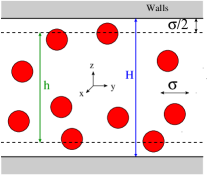
(a)

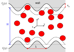
(b)

Figure 1: Schematics of the geometries of the confined fluid system, as described in the text. (a) Featureless walls and (b) physically rough walls.

We study the hard-sphere fluid confined between parallel hard walls in a slit-pore geometry. To avoid any confusion, we point out that none of the walls studied here exhibits internal structure. That is, the walls are of uniform density and can be regarded as a continuum solid. Let $H$ denote the average distance between the two surfaces of the confining walls. In this work, we study two general types of wall surfaces. The first involves flat walls where the boundary conditions for the particle-wall collisions have been modified. These walls model surface roughness on a length scale much smaller than the diameters of fluid particles, and thus, because the surfaces are geometrically flat, they are referred to as featureless surfaces (walls). The second type of surface studied here possesses physical (i.e., geometric) roughness, i.e., the height of the wall surface varies with lateral position, and thus they are referred to as physically rough surfaces (walls). Schematics of each type of surface are given in Fig. 1.

III.1 Featureless Walls

We considered three different types of boundary conditions for particle collisions with featureless walls. As a useful reference state, we first considered flat, smooth walls (SW), where the fluid-wall collisions are specular. The second type of featureless surface studied was a so-called thermal wall (TW). This model boundary attempts to reproduce particle collisions with a surface uneven on length scales considerably smaller than the particle diameter, the essential feature being that pre- and post-wall collision velocities are uncorrelated. More importantly, the distribution of post- collision velocities is determined by the temperature of the wall. The third type of featureless surface gives an alternative approach to generate uncorrelated pre- and post-wall-collision velocities. We refer to it as a rotational wall (RW) for reasons that will become apparent below.

In order to distinguish between the featureless walls with different boundary conditions, consider a particle with a pre-wall-collision velocity $\mathbf{v}=(v_{x},v_{y},v_{z})$, and a post-wall collision velocity $\mathbf{v}^{\prime}=(v_{x}^{\prime},v_{y}^{\prime},v_{z}^{\prime})$. For the cases considered here, the components of $\mathbf{v}^{\prime}$ are as follows.

• Smooth walls (SW): $v^{\prime}_{x}=v_{x}$, $v^{\prime}_{y}=v_{y}$, and $v^{\prime}_{z}=-v_{z}$

• Thermal walls (TW): $v_{z}^{\prime}$ is chosen according to the following distributionTehver et al. (1998) depending on wall temperature $T_{\mathrm{w}}$ (set equal to fluid temperature $T$):

  $$\phi_{z}(v_{z}^{\prime})=\frac{m}{k_{B}T_{w}}\ \lvert v_{z}^{\prime}\rvert\ \exp{\left[\frac{-mv_{z}^{\prime 2}}{2k_{B}T_{\mathrm{w}}}\right]}$$ (2)

  where the sign of $v_{z}^{\prime}$ depends on the location of the wall collision (i.e., positive for lower wall collisions and negative for upper wall collisions). $v_{i}^{\prime}$ (where $i=x,y$) is chosen randomly from a Gaussian distribution:

  $$\phi_{i}(v_{i}^{\prime})=\sqrt{\frac{m}{2\pi k_{B}T_{\mathrm{w}}}}\ \exp{\left[\frac{-mv_{i}^{\prime 2}}{2k_{B}T_{w}}\right]}$$ (3)

• Rotational walls (RW): $v^{\prime}_{z}=-v_{z}$, and the lateral components $v^{\prime}_{x}$ and $v^{\prime}_{y}$ are determined by rotating the corresponding components of the pre-wall-collision velocity $v_{x}$ and $v_{y}$ by an angle $\theta$:

  $$\begin{split}v_{x}^{\prime}&=v_{x}\cos\theta^{\prime}-v_{y}\sin\theta^{\prime}\\ v_{y}^{\prime}&=v_{x}\sin\theta^{\prime}+v_{y}\cos\theta^{\prime},\end{split}$$ (4)

  where $\theta^{\prime}=\pm\theta$, with the sign chosen randomly. Note that $\theta=0$ corresponds to smooth walls, while $\theta=\pi$ corresponds to bounce-back boundary conditions.

Note that the boundary conditions described above affect the dynamics of the system only. Because all three of the above walls have the same geometrical form and produce the same velocity component distributions, they lead to identical thermodynamic and structural properties Tehver et al. (1998). This was verified by the simulation results.

We note that the featureless walls described above are not intended to model any specific physical system. Rather, they are mathematically convenient course-grained models for surface roughness. For example, the motivation for the thermal walls goes back to Maxwell Maxwell (1867), who considered collisions with a highly uneven low density granular surface. Particles that strike this type of surface undergo a series of collisions with many different surface molecules. The resulting outgoing velocity is expected to be randomized, with a distribution determined by the temperature of the wall. We also stress that the rotational walls introduced here are not intended to mimic any type of real system. Instead, they should be considered a mathematical construct that allows us to change the surface boundary condition in a continuous fashion from perfectly smooth ($\theta=0$) to rough (bounce-back, $\theta=\pi$) walls, with the system having identical thermodynamics for all values of $\theta$. This allows us to study how different levels of surface roughness impact the dynamics of the model fluid without changing thermodynamics.

III.2 Physically rough walls

For a physically rough surface, we intuitively expect that the height of the surface should vary with lateral position. For simplicity, we use the following expressions for the upper and lower wall surfaces in a slit- pore geometry:

$$\begin{split}f_{\rm{U}}(y)&=\frac{H}{2}+a_{w}\cos\left[\frac{2\pi y}{\lambda}+\pi\right],\\ f_{\rm{L}}(y)&=-\frac{H}{2}+a_{w}\cos\left[\frac{2\pi y}{\lambda}\right]\end{split}$$ (5)

where the subscripts $\rm{L}$ and $\rm{U}$ denote the lower and upper surfaces, respectively, and $a_{w}$ and $\lambda$ are the amplitude and wavelength of the well-behaved surface variations, respectively. Figure 1b displays the geometry of the physically rough walls employed. As written in Eq. (5) and depicted in Figure 1b, minima in the upper wall and maxima in the lower wall are aligned, which imposes a maximum value upon $a_{w}$ if a fluid particle is to have access to the entire pore length. The average surface-to-surface distance is $H$ as long as the quantity $L_{y}/\lambda$ is an integer, which is true throughout this work. Because we have chosen to have the height of the surface be a function of only $y$, the system is spatially inhomogeneous in the $y$-direction and homogeneous in the $x$-direction. This will have important consequences for the self diffusivity of a fluid confined between these surfaces.

The rigid character of the confining walls was maintained by requiring perfectly reflecting specular particle-surface collisions. However, instead of solving the set of nonlinear equations to determine particle-surface collision times, which is computationally expensive, the curved walls were discretized into a set of short, connected line segments of length $0.015\sigma$. Using smaller segments does not lead to noticeable changes in the resulting properties of the systems studied here.

We stress that the specific form of the physically rough walls studied here is not intended to mimic a specific physical system. Rather, they allow us to systematically determine the impact of different surface feature sizes on the self-diffusivity of our model fluid.

IV Results

IV.1 Featureless Flat Walls

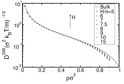
Figure 2: Self diffusivity $D$ versus total density $\rho=N/(AH)$ for the hard-sphere fluid confined between smooth walls in slit-pore geometry.

We first present results for the hard-sphere fluid confined between smooth, flat hard walls. In Fig. 2, we plot the self-diffusion coefficient, $D^{\rm{SW}}$, where the superscript SW signifies smooth wall case, as a function of the total density $\rho=N/(AH)$. Data are shown for a number of pore widths $H$. As previously pointed out elsewhereMittal et al. (2006); Goel et al. (2009), all data points seem to fall approximately onto a single curve independently of $H$ for $\rho\sigma^{3}\lesssim 0.75$. Below, we investigate how modifying the nature of the confining surfaces changes the results obtained in this basic reference system.

IV.2 Thermal Walls

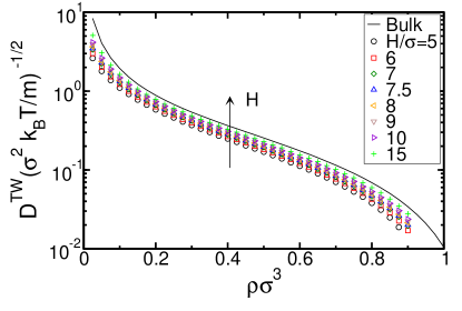
Figure 3: Self diffusivity $D$ versus total density $\rho$ for the hard-sphere fluid confined between thermal walls, for various wall separations $H$.

Figure 3 displays the self-diffusion coefficient $D^{\rm{TW}}$ for the hard-sphere fluid confined between featureless thermal walls as a function of $\rho$ for various values of $H$. Compared to the smooth, flat wall, roughness due to the thermal wall has a clear and noticeable influence on particle dynamics. Thermal walls reduce particle mobility, with the magnitude of the reduction increasing with decreasing $H$. That average mobility of fluid particles confined between thermal walls decreases with $\rho$ at fixed $H$ has been previously reported.Subramanian and Davis (1979)

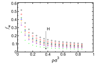
Figure 4: Fraction of collisions in the system involving the wall surface $f_{w}$ for the hard-sphere fluid confined to a slit-pore geometry. Symbols have the same meaning as in Fig. 3

The interesting trend we quantify in this study is the reduction of $D^{\rm{TW}}$ with increasing degree of confinement at fixed $\rho$. This behavior can be understood by considering the quantity $f_{w}$, the fraction of collisions in the system involving the surfaces of the confining walls. Intuitively, we expect non-specular particle-surface collisions, such as those that take place in the thermal-wall systems, to slow dynamics in the transverse direction relative to specular particle-surface collisions. We base this expectation by considering the free flight of a single particle. In this case, specular particle-wall collisions do not change the transverse motion, while non-specular particle-wall collisions do. We also expect that the fraction of wall collisions grows with the prominence of the walls (the fraction of the fluid particles near the walls), that is, with decreasing $H$. That is, in order to maintain a fixed $N$ and $V$, a decrease in $H$ must be compensated by an increase in fluid-exposed wall surface area. Figure 4 shows that this is indeed the case. Decreasing $H$ at constant $\rho$ systematically increases the fraction of wall collisions. Clearly, the reduction in $D^{\rm{TW}}$ with decreasing $H$ observed in Fig. 3 is directly linked to the increasing fraction of wall collisions. Also, note that the results given in Fig. 4 are not unique to the thermal-wall systems. In fact, all three kinds of featureless surfaces studied in this work yield identical wall-collision statistics. As noted above, the collision boundary conditions only affect the dynamic properties of the fluid and not the thermodynamic properties. The thermodynamic pressure of the system is intimately related to the wall-collision statistics.

While there are clear differences between the smooth-wall and thermal-wall self-diffusion coefficients, $D^{\rm{SW}}$ and $D^{\rm{TW}}$, respectively, these differences appear to depend systematically on $H$. This suggests that it might be possible to develop an approach to predict the self-diffusivity of the hard-sphere fluid confined between thermal walls using a limited amount of information. In particular, note the dependence of the fraction of wall collisions on density. Initially, increasing density leads to a pronounced decrease in the fraction of wall collisions. This is due to the associated increase in particle-particle collisions compared to particle-wall collisions (not shown). However, the fraction of wall collisions eventually becomes a weak function of density. Since we expect the reduction in self diffusivity due to the presence of rough walls to scale with the fraction of wall collisions, we should likewise expect a similar density dependence of the ratio $D^{\rm{TW}}/D^{\rm{SW}}$.

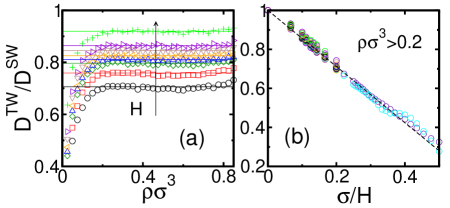
(a)

(b)

Figure 5: Ratio of the self-diffusivity between thermal walls $D^{\rm{TW}}$ to its value when confined between smooth walls $D^{\rm{SW}}$ at the same $\rho$ and $H$ versus (a) $\rho$ and (b) $H^{-1}$. Symbols in (a) are the same as those in Fig. 3. In (b), all data is for $\rho\sigma^{3}>0.2$, and dashed line is a fit to the form $D^{\rm{TW}}/D^{\rm{SW}}=1.0-1.44\sigma/H$.

In Fig. 5a, we plot the quantity $D^{\rm{TW}}/D^{\rm{SW}}$ as a function of density. The ratio of the diffusivities is taken at the same thermodynamic state of the fluid, namely at the same density $\rho$ and average wall separation $H$. Notice that, for each pore width, the ratio of self-diffusion coefficients initially increases with density before reaching a limiting value. Furthermore, the behavior of $D^{\rm{TW}}/D^{\rm{SW}}$ vs $\rho$ reflects that of $f_{w}$ vs $\rho$. Again, this points to the strong connection between the self-diffusion in a system with rough walls to the prominence of the walls (i.e., the fraction of the fluid near the walls). The diffusivity ratio takes its smallest value at low density, conditions where surface collisions are most influential, and thus, where the greatest difference between the two surfaces is observed. Also, the density at which the ratio reaches a plateau value ($\rho\sigma^{3}\approx 0.2$) is independent of pore width. This is due to the dominant influence of particle-particle collisions on the mobility of hard-spheres at moderate-to-high densities.

The most striking feature of Fig. 5a involves the $H$-dependent plateau values for $\rho\sigma^{3}\gtrsim 0.2$. In Fig. 5b, we plot all of the data points for which $\rho\sigma^{3}\gtrsim 0.2$ versus the inverse pore width $H^{-1}$. Fig. 5b shows that the ratio of diffusivities can be well described in this density range by a linear function of $H^{-1}$

$$\frac{D^{\rm{rough}}}{D^{\rm{ref}}}=1-C\left(\frac{\sigma}{H}\right),$$ (6)

where the constant $C$ is a fitting parameter, $D^{\rm{rough}}$ is the self-diffusivity of the fluid between the rough surface of interest, and $D^{\rm{ref}}$ is the self diffusivity of the fluid at an appropriately chosen reference state under the same thermodynamic conditions. We note that Eq. (6) has, to first order, the same dependence on $H$ as the self-diffusivity of a Brownian particle in the center of a slit-pore.Happel and Brenner (1983) This, in fact, was the inspiration for the functional form chosen in Eq. (6). For the thermal walls, we take $D^{\rm{rough}}=D^{\rm{TW}}$ and $D^{\rm{ref}}=D^{\rm{SW}}$, and we find that $C\approx 1.44\sigma$.

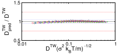
Figure 6: Ratio of predicted to observed self diffusivity (see text) for the thermal wall system. Dotted blue and red dashed lines provide $5\%$ and $25\%$ error bounds, respectively. Symbols are the same as those in Fig. 3.

Assuming sufficient smooth-wall self-diffusivity data are available as a function of density, this provides the basis for estimating the diffusivity of the hard-sphere fluid confined between thermal walls for $\rho\sigma^{3}>0.2$. To estimate the diffusivity of a fluid confined between thermal walls in a slit pore of width $H$ at density $\rho$, one calculates two quantities. The first quantity is the $H$-dependent ratio $D^{\rm{TW}}/D^{\rm{SW}}$ using Eq. 6, and the second quantity is the self-diffusion coefficient of the reference system, $D^{\rm{SW}}$, which, as discussed in Section I, may be approximated by a scaling analysis. Knowledge of these two quantities then allows for an estimate of the self diffusivity between thermal walls. In Fig. 6, we test the predictive ability of this approach. The ratio of the predicted to observed thermal wall self diffusivity is plotted against the observed self diffusivity for the thermal-wall system. If the predictions were perfect, the points would fall on the horizontal line $D^{\rm{TW}}/D^{\rm{SW}}=1$, and this is clearly not the case. However, the predicted data points do fall within the indicated $5\%$ error bounds. Moreover, we emphasize that to truly make predictions, one must still have knowledge of $C$ and the reference self-diffusivity.

IV.3 Rotational walls

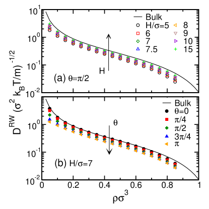
(a)

(b)

Figure 7: Self diffusivity $D^{\rm{RW}}$ versus density $\rho$ for the hard-sphere fluid confined between rotational walls at (a) $\theta=\pi/2$ and various wall separations $H$ and (b) $H/\sigma=7$ and various values of $\theta$.

In Figure 7, we present results for the self-diffusion coefficient $D^{\rm{RW}}$ of the hard-sphere fluid confined between rotational walls as a function of density $\rho$ with (a) $\theta=\pi/2$ and various values of $H$, and (b) $H/\sigma=7.0$ and various values of $\theta$. Qualitatively similar results were observed for other choices of rotational-wall parameters and can be found in Supplementary Materials.sup Recall that $\theta$ is the angle of rotation that the lateral velocity of a particle undergoes after it collides with the surface. Fig. 7a shows that self diffusivity decreases with increasing density at fixed $H$ and fixed $\theta$. In addition, at fixed density $\rho$, the self-diffusivity decreases with decreasing $H$. This latter trend, which was also observed in the the thermal-wall systems, is not surprising considering rotational walls, like thermal walls, inherently retard particle mobility, an effect that is most apparent at small wall separations (at the same fluid density). Therefore, recalling that the collision statistics are independent of the boundary condition for featureless walls, the same physics explaining the reduction in mobility due to thermal walls mentioned in Section IV.2 also applies to rotational walls. We also expect that the reduction in mobility should increase with $\theta$, since $\theta$ controls the effective roughness of the walls. The data presented Figure 7b bear this out.

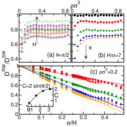
(a)

(b)

(c)

Figure 8: Ratio of self diffusivity between rotational walls $D^{\rm{RW}}$ to that between smooth walls $D^{\rm{SW}}$ at the same $\rho$ and $H$ versus $\rho$ at (a) $\theta=\pi/2$ and various $H$ and (b) $H/\sigma=7$ and various $\theta$, and versus (c) $H^{-1}$ at various $\theta$. Symbols in (a) and (b-c) are the same as those in Figs. 7a and 7b, respectively. In (c), all data points are for $\rho\sigma^{3}>0.2$; lines are linear fits of the form $D^{\rm{RW}}/D^{\rm{SW}}=1-C(H/\sigma)^{-1}$; the inset to (c) shows the value of $C$ as a function of $\theta$ from linear fits in main panel of (c).

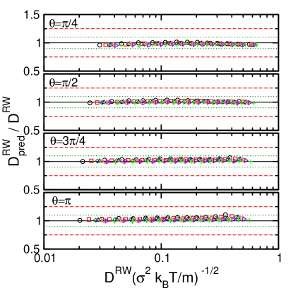
Figure 9: Ratio of predicted to observed self diffusivity (discussed in text) versus the observed self diffusivity for the rotational wall system with the value of $\theta$ denoted in each figure. Dotted blue and red dashed lines provide $10\%$ and $25\%$ error bounds, respectively. Symbols have the same meaning as in Fig. 7a.

Figures 8a and 8b again show that rotational walls influence self diffusivity relative to smooth walls in a manner qualitatively similar to thermal walls. Specifically, the ratio of self diffusion coefficients $D^{\rm{RW}}/D^{\rm{SW}}$ initially increases with density and then levels off beyond $\rho\sigma^{3}\gtrsim 0.2$. In fact, for a given $\theta$, the plateau value appears to be systematically dependent upon $H$, which suggests that an approach similar to that adopted for the thermal wall system can be used to estimate the diffusivity in the rotational-wall system. Figure 8b shows that the ratio $D^{\rm{RW}}/D^{\rm{SW}}$ decreases with increasing $\theta$, indicating that the constant $C$ in Eq. (6) is dependent upon $\theta$. This just reflects the $\theta$ dependence noted in Fig. 7b. Accounting for this $\theta$ dependence, Fig. 8c shows that diffusivity ratios with densities $\rho\sigma^{3}>0.2$ are well described by Eq. (6). The inset to Fig. 8c displays the values of $C(\theta)$ from the fits. For simplicity, we fit $C$ to the function $C=2.0sin(\theta/2)$, which as shown in Fig. 8c fits the data well. specific form of the fit was based on the fact that $C=0$ for $\theta=0$ (by definition), $C$ is a maximum at $\theta=\pi$, and $C$ is periodic in $\theta$. Using the procedure outlined above for thermal walls, the self-diffusion of the hard-sphere fluid between rotational walls can be estimated in an analogous fashion. Figure 9 tests these estimates, plotting the ratio $D^{\rm{RW}}_{\mathrm{pred}}/D^{\rm{RW}}$ versus $D^{\rm{RW}}$, where $D^{\rm{RW}}_{\mathrm{pred}}$ is the predicted value and $D^{\rm{RW}}$ is the value observed from simulation. In the case of rotational walls, the estimation procedure yields predictions that fall within $10\%$ of the actual values. More accurate predictions can clearly be obtained by making use of a more quantitative model for $C(\theta)$.

IV.4 Physically rough walls

Here, we present results for physically rough surfaces at fixed wavelength $\lambda/\sigma=3$ and several densities $\rho=N/V$, where $V$ is the surface accessible volume, while (1) fixing the amplitude of the features $a_{w}/\sigma=1.0$ and varying $H$ and (2) fixing $H/\sigma=7.5$ and varying $a_{w}$. Since the surface height of a physically rough wall depends on lateral position, these parameters (see Eq. 5 and Fig. 1b) allow us to study the influence of surface height variation on mobility in a systematic way. Results for $\lambda/\sigma=1.5$, $2.0$, and $6.0$ give results qualitatively similar to those presented below, and can be found in Supplementary Materials.sup

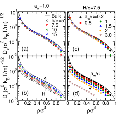
(a)

(b)

(c)

(d)

Figure 10: Self diffusivity in (a,c) smooth $x$ and (b,d) rough $y$ directions versus density for the hard-sphere fluid confined between physically rough walls (see Fig. 1b) with $\lambda/\sigma=3.0$ and (a,b) $a_{w}/\sigma=1.0$ and various $H$ and (c,d) $H/\sigma=7.5$ and various $a_{w}$.

Notice that in the geometry of the physically rough wall system studied (see Fig. 1b), the $x$ and $y$ directions, though both infinite, are not equivalent. Because the surface height is a function of $y$ only, the $y$ direction is termed rough (inhomogeneous), while the $x$ direction is termed smooth (homogeneous). Also, because of this height variation, we expect the self diffusivities in the $x$ and $y$ directions at the same state point to be significantly different, with $D_{x}>D_{y}$. Figure 10 shows these two self-diffusion coefficients separately as a function of density for various values of $H$ and $a_{w}$. Observe that the self diffusivity in the $x$ direction has little dependence on $H$ or $a_{w}$. That is, the $D_{x}$–$\rho$ correlation is almost equivalent to the bulk correlation, much like the case for hard spheres between smooth flat walls (see Fig. 2). This seems consistent with previous results for hard-spheres in cylindrical pores where the surface is smooth and exhibits curvature.Goel et al. (2009)

In contrast, the self-diffusion coefficient in the $y$ direction depends strongly on the degree of confinement (Fig. 10b) and on the amplitude $a_{w}$ of the surface variation (Fig. 10d). Specifically, decreasing $H$ at fixed wall feature size (constant $a_{w}$ and $\lambda$) systematically decreases $D_{y}$. This behavior resembles that for the fluid confined between thermal walls (Fig. 3) and rotational walls (Figs. 7a). Also, at fixed $H$, $D_{y}$ systematically decreases with increasing $a_{w}$ (i.e., increasing surface roughness). This effect is analogous to increasing surface roughness ($\theta$) in the rotational wall system (see Fig. 7b). Also, the slowing down of dynamics due to physical roughness is consistent with previous studies.Sofos et al. (2010)

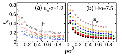
(a)

(b)

Figure 11: Fraction of particle collisions that involve the wall $f_{w}$ for the hard-sphere fluid confined between physically rough walls versus density. (a) $a_{w}/\sigma=1.0$ at various $H$ and (b) $H/\sigma=7.5$ and various $a_{w}$. Symbols have the same meaning as in Fig. 10.

The disparity between $D_{x}$ and $D_{y}$ grows with decreasing $H$ at fixed $a_{w}$ and $\lambda$, and with increasing roughness ($a_{w}$) and fixed $H$. Given the close parallels between $D_{y}$ and the self-diffusion coefficient of the fluid between featureless rough walls, we expect the reduction in $D_{y}$ due to surface roughness should be connected to the fraction of collisions in the system involving the walls. In Figure 11, we plot $f_{w}$ versus density for the state points considered in Fig. 10. Fig. 11a shows that $f_{w}$ grows with decreasing $H$ at fixed $\rho$ and $a_{w}$, while Fig. 11b shows that the wall-collision fraction grows with $a_{w}$ at fixed $\rho$ and $H$. In both cases, $f_{w}$ grows with the increasing prominence of the walls (caused by decreasing $H$, or increasing $a_{w}$) Also, at fixed wall conditions (e.g., $a_{w}$ and $\lambda$), $f_{w}$ initially decreases with increasing density ($\lesssim 0.2$). However, this quantity changes only moderately with further increases in density ($\gtrsim 0.2$). This behavior is analogous to that observed in the featureless-wall systems.

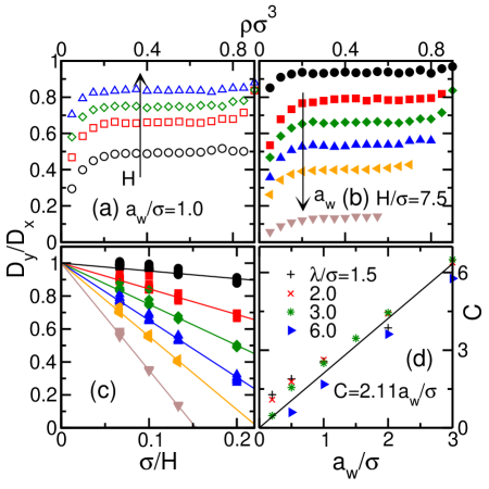
(a)

(b)

(c)

(d)

Figure 12: Ratio of self diffusivity in rough direction $D_{y}$ and smooth direction $D_{x}$ with $\lambda/\sigma=3.0$ versus (a,b) $\rho$ and (c) $H^{-1}$ for the hard-sphere fluid confined between physically rough walls. Symbols in (a-c) are the same as in Fig. 10. In (c) all data points are for $\rho\sigma^{3}>0.2$ and lines are fits to the form $D_{y}/D_{x}=1-C(H/\sigma)^{-1}$. Panel (d) displays the values of $C$ versus $a_{w}$ at all the wavelengths studied.

Because of the qualitative similarities between the properties of the physically rough-wall system and the featureless rough-wall systems studied above, we now examine the diffusivity ratio $D_{y}/D^{\rm{ref}}$. However, unlike the other surfaces encountered in this work, the choice of $D^{\rm{ref}}$ is not obvious for the physically rough walls. For the thermal and rotational walls, we chose the smooth (flat) wall self-diffusion coefficient at the same $\rho$ and $H$, which corresponds to the self-diffusion of a fluid at the same thermodynamic state without surface roughness. Likewise, for physically rough-wall system, the reference state should be the self-diffusion of a system at the same thermodynamic state, but without surface roughness. For this, we choose $D^{\rm{ref}}=D_{x}$. In Figure 12a, we plot the ratio $D_{y}/D_{x}$ versus density for various values of $H$ and $a_{w}$. At fixed $H$, the ratio initially increases with $\rho$ and then levels off beyond $\rho\sigma\gtrsim 0.2$. For a specified value of $\rho$, the ratio $D_{y}/D_{x}$ decreases with decreasing $H$ at fixed surface roughness (Fig. 12a) and with increasing roughness at fixed $H$ (Fig. 12b). Comparison with Figs. 5a and 8 shows that physical roughness alters $D_{y}$ relative to $D_{x}$ in a manner similar to how featureless rough walls alter the self-diffusion relative to smooth walls. Figure 12c shows that, for given surface features, $D_{y}/D_{x}$ is a linear function of $H^{-1}$. That is, $D_{y}$ follows Eq. (6) with $D^{\rm{rough}}=D_{y}$ and $D^{\rm{ref}}=D_{x}$. Figure 12d shows the fit parameter $C$ versus $a_{w}$ for the different surface feature wavelengths $\lambda$ studied (see Supplementary materialsup ). Clearly, $C$ is much more sensitive to $a_{w}$ than $\lambda$. We find that a linear fit to $C$ as a function of $a_{w}$, although crude, describes that data reasonably well.

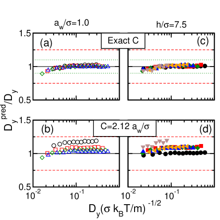
(a)

(b)

(c)

(d)

Figure 13: Ratio of predicted $D^{\mathrm{pred}}_{y}$ (see text) to observed value of $D_{y}$ plotted versus $D_{y}$ for the hard-sphere fluid confined between physically rough walls with $\lambda/\sigma=3.0$ and (a,b) $a_{w}/\sigma=1$ and various $H$ and (c,d) $H/\sigma=7.5$ and various $a_{w}$. Symbols in (a,b) and (c,d) correspond to those in Figs. 10a and 10c, respectively. In (a,c) we use values of $C$ obtained from the fits in Fig. 12c, while in (b,d) we use $C=2.12a_{w}/\sigma$ (see Fig. 12d). The dotted green and dashed red lines correspond to $10\%$ and $25\%$ error bounds, respectively.

From the above analysis, we can now formulate a means to predict the self-diffusion in the rough $y$ direction from the self diffusion in the smooth $x$ direction. Specifically, from Eq. (6), $D_{y}^{\mathrm{pred}}=D_{x}[1-C\,(H/\sigma)^{-1}]$. Figure 13 shows the quality of the prediction based on this formalism for the state points in Fig. 10. In Figs. 13a,LABEL:sub@fig:DY_prediction_exact_h_7p5 we use $C$ from the fits at a given $\lambda$ (i.e., data points in Fig. 12d), while in Figs. 13b,LABEL:sub@fig:DY_prediction_approx_h_7p5 we use the approximation $C=2.12a_{w}/\sigma$ (linear fit in Fig. 12d). We find that using the $C$ for a given wall configuration yields good predictions, with the majority of the data within $10\%$ of the actual data. On the other hand, using the approximate $C$ yields predictions within $25\%$ of the actual value. The information necessary to estimate $D_{y}$ in this case is greatly reduced, but one would still need knowledge of $D_{x}$ to truly make predictions of $D_{y}$.

V Conclusions

We have systematically studied how surface roughness affects the self-diffusion of confined hard-sphere fluids. Specifically, for $\rho\sigma^{3}>0.2$, we have shown that the ratio of the self-diffusion coefficient in a rough wall system to the self-diffusion coefficient in smooth-wall reference system is a linear function of reciprocal wall separation [see Eq. (6)], with the precise slope depending on the specific nature of the surface roughness. If this slope and the reference self-diffusivity are known, accurate predictions of the self-diffusion in rough wall systems can be obtained.

In real world applications, however, the specific nature of surface roughness is often unknown. This study leads to two possible ways of making useful self-diffusivity estimates without this knowledge. First, our analysis shows that a only a limited number of measurements are needed to determine $C$. Second, if only qualitative information is sought, our analysis shows that $C$ is typically of $O(1)$, and that the basic physics of self-diffusion in a rough system relative to that in a smooth system is captured by the $H^{-1}$ correction in Eq. (6). That is, the specific nature of the surface roughness does not appear to impact radically or significantly the resulting dynamics. This is particularly important since modeling the specific details of real surfaces is a daunting task. However, it is not our intention to suggest that any type of surface roughness can be modeled in any way one chooses, for example, modeling geometric roughness with featureless rough walls. Rather, the specific details of the surface roughness do not appear to be overly important.

To make predictions for self-diffusion of confined fluids between rough surfaces using Eq. (6), one also requires a prediction of the reference state self-diffusion. As discussed in Section I, one may use a scaling method to map the bulk system to the confined system. For the case of smooth featureless walls, for example, this has been shown to be very effective.Goel et al. (2009) However, for the case of the physically rough system, one must be able to predict $D_{x}$. We plan to address this in a future publication.

Another question is whether the results presented in this paper apply to more complex pore scenarios, such as diffusion through porous materials. Such systems have complex geometry and connectivity, as well as rough surfaces. We believe that the simplified geometry studied here, slit pores, is applicable, however, when one considers that many of the properties in such complex systems can be considered as an average over a collection of simple slit pore (or cylindrical pore) systems. Lastoskie et al. (1993); Olivier et al. (1994); Lastoskie et al. (1997); Rouquerol and Rouquerol (1999); Klobes et al. (2006)

The lack of particle-particle or particle-wall attractions is an obvious shortcoming of this study. Clearly, wall attractions will greatly alter the number of particles near the wall, and therefore the fraction of wall collisions. As we point out, the ratio of self diffusivity in a rough-wall system to that in a corresponding smooth-wall system appears to be closely linked with the fraction of wall collisions. Therefore, attractions can have a strong effect on the behavior of the self diffusivity ratio. However, we speculate that the introduction of moderately strong wall attractions to the rough systems studied here will result in an increased retardation of self-diffusion and not a fundamental change to the physics. We also plan to explore this issue in detail in a future publication.

Figure Captions

Rotational walls

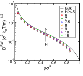
(a)

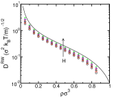
(b)

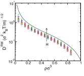
(c)

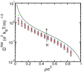
(d)

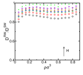
(e)

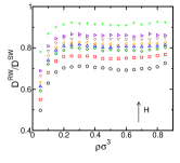
(f)

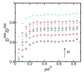
(g)

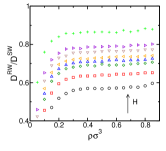
(h)

Figure 14: Properties for rotational walls. (a-d) Self-diffusion versus density. (e-h) Ratio of the self-diffusion between rotational walls and between smooth walls at some $H$ and $\rho$ versus density. Values of $\theta$ are indicted above each figure.

Physically rough walls

(a)

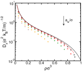
(b)

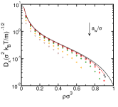
(c)

(d)

(e)

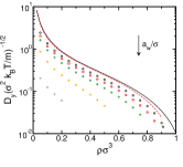
(f)

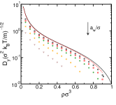
(g)

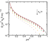
(h)

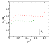
(i)

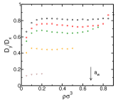
(j)

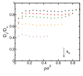
(k)

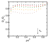
(l)

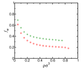
(m)

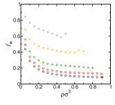
(n)

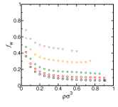
(o)

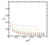
(p)

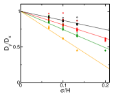
(q)

Figure 15: Self-diffusion for physically rough system with $\lambda/\sigma=1.5$. (a-d) Self-diffusion in $x$ direction $D_{x}$, (e-h) self-diffusion in $y$ direction $D_{y}$, (i-l) $D_{y}/D_{x}$, and (m-p) fraction of wall collisions $f_{w}$ vs density. (q) $D_{y}/D_{x}$ vs $H^{-1}$ for points with $\rho\sigma^{3}>0.2$.

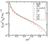
(a)

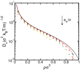
(b)

(c)

(d)

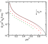
(e)

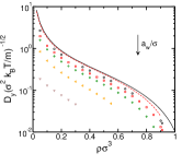
(f)

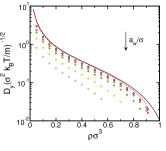
(g)

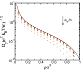
(h)

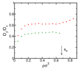
(i)

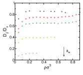
(j)

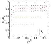
(k)

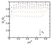
(l)

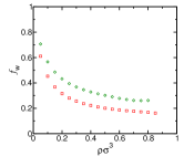
(m)

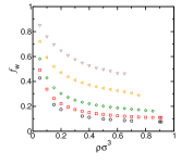
(n)

(o)

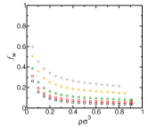
(p)

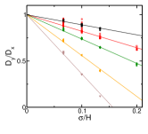
(q)

Figure 16: Same as Fig. 15 with $\lambda/\sigma=2.0$.

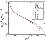
(a)

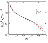
(b)

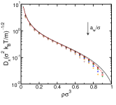
(c)

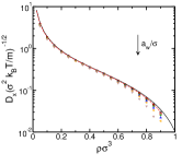
(d)

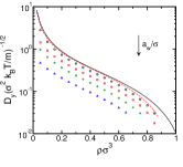
(e)

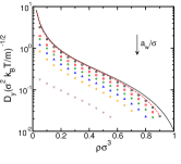
(f)

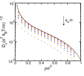
(g)

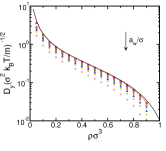
(h)

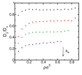
(i)

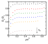
(j)

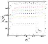
(k)

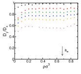
(l)

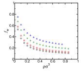
(m)

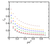
(n)

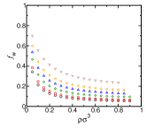
(o)

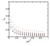
(p)

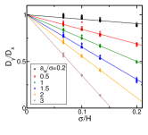
(q)

Figure 17: Same as Fig. 15 with $\lambda/\sigma=3.0$.

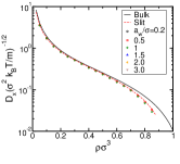
(a)

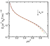
(b)

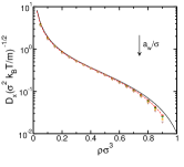
(c)

(d)

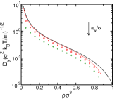
(e)

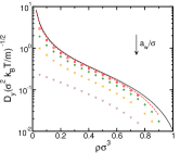
(f)

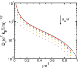
(g)

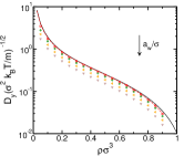
(h)

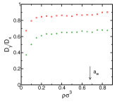
(i)

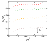
(j)

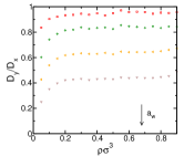
(k)

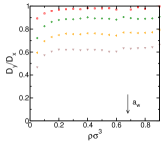
(l)

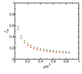
(m)

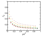
(n)

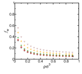
(o)

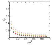
(p)

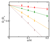
(q)

Figure 18: Same as Fig. 15 with $\lambda/\sigma=6.0$.

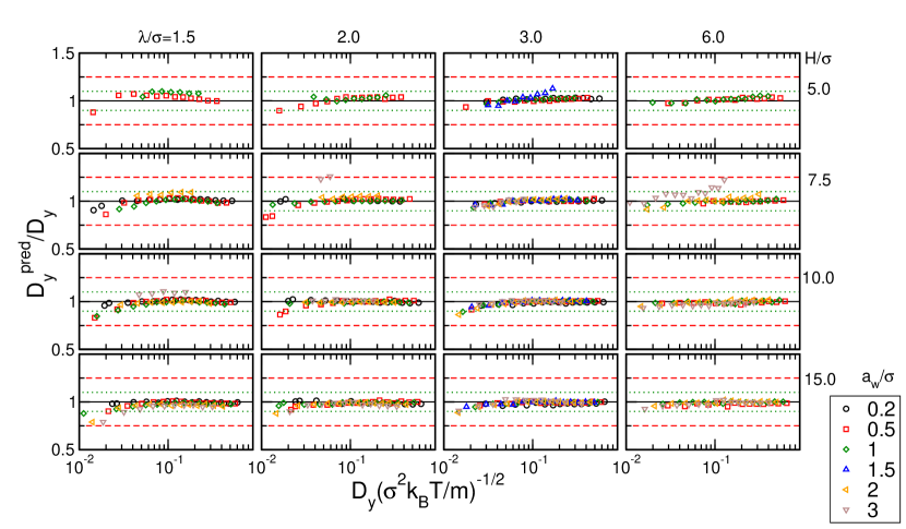
(a)

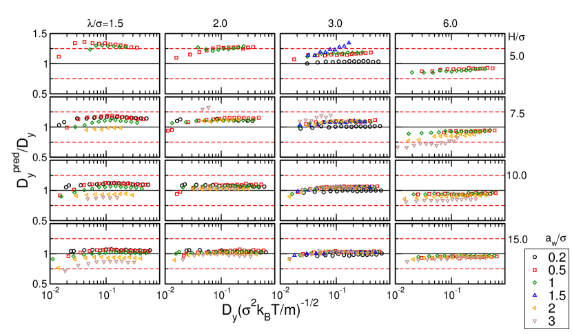
(b)

Figure 19: Ratio of predicted value of $D_{y}$ from $D_{y}/D_{x}=1-C[H/\sigma]^{-1}$ to actual value of $D_{y}$ versus $D_{y}$ for states with $\rho\sigma^{3}>0.2$. In (a), values of $C$ used in prediction are taken from the full linear fits shown in subfigure (q) of the above figures. In (b), the value of $C$ is taken from the linear fit $C=2.12a_{w}/\sigma$ (see main text). The dotted green and dashed red lines correspond to $10\%$ and $25\%$ error bounds, respectively.

References and Notes

- Bhushan et al. (1995) B. Bhushan, J. N. Israelachvili, and U. Landman, Nature 374, 607 (1995).
- Mittal et al. (2006) J. Mittal, J. R. Errington, and T. M. Truskett, Phys. Rev. Lett. 96, 177804 (2006).
- Mittal et al. (2007a) J. Mittal, J. Errington, and T. Truskett, J. Phys. Chem. B 111, 10054 (2007a).
- Mittal et al. (2007b) J. Mittal, J. R. Errington, and T. M. Truskett, J. Chem. Phys. 126, 244708 (2007b).
- Mittal et al. (2007c) J. Mittal, V. K. Shen, J. R. Errington, and T. M. Truskett, J. Chem. Phys. 127, 154513 (2007c).
- Goel et al. (2008) G. Goel, W. P. Krekelberg, J. R. Errington, and T. M. Truskett, Phys. Rev. Lett. 100, 106001 (2008).
- Mittal et al. (2008) J. Mittal, T. M. Truskett, J. R. Errington, and G. Hummer, Phys. Rev. Lett. 100, 145901 (2008).
- Goel et al. (2009) G. Goel, W. P. Krekelberg, M. J. Pond, J. Mittal, V. K. Shen, J. R. Errington, and T. M. Truskett, J. Stat. Mech. 2009, P04006 (2009).
- Mittal (2009) J. Mittal, J. Phys Chem. B 113, 13800 (2009).
- Chopra et al. (2010) R. Chopra, T. M. Truskett, and J. R. Errington, Phys. Rev. E 82, 041201 (2010).
- Grzelak et al. (2010) E. M. Grzelak, V. K. Shen, and J. R. Errington, Langmuir 26, 8274 (2010).
- Grzelak and Errington (2010) E. M. Grzelak and J. R. Errington, Langmuir 26, 13297 (2010).
- Knudsen (1909) M. Knudsen, Ann. Phys. (Leipzig) 28, 75 (1909).
- Arya et al. (2003) G. Arya, H.-C. Chang, and E. J. Maginn, Phys. Rev. Lett. 91, 026102 (2003).
- Malek and Coppens (2001) K. Malek and M. Coppens, Phys. Rev. Lett. 87, 125505 (2001).
- Malek and Coppens (2002) K. Malek and M. Coppens, Colloid Surface A 206, 335 (2002).
- Malek and Coppens (2003) K. Malek and M.-O. Coppens, J. Chem. Phys. 119, 2801 (2003).
- Edmond et al. (2010) K. V. Edmond, C. R. Nugent, and E. R. Weeks, Eur. Phys. J.-Spec. Top. 189, 83 (2010).
- Scheidler et al. (2002) P. Scheidler, W. Kob, and K. Binder, Europhys. Lett. 59, 701 (2002).
- Scheidler et al. (2004) P. Scheidler, W. Kob, and K. Binder, J. Phys Chem. B 108, 6673 (2004).
- Errington et al. (2003) J. R. Errington, P. G. Debenedetti, and S. Torquato, J. Chem. Phys. 118, 2256 (2003).
- Hansen and McDonald (2006) J. P. Hansen and I. R. McDonald, Theory of Simple Liquids (Academic, London, 2006), 3rd ed.
- Lastoskie et al. (1993) C. Lastoskie, K. E. Gubbins, and N. Quirke, J. Phys. Chem. 97, 4786 (1993).
- Olivier et al. (1994) J. Olivier, W. Conklin, and M. Szombathely, Stud. Surf. Sci. Catal. 87, 81 (1994).
- Lastoskie et al. (1997) C. Lastoskie, N. Quirke, and K. Gubbins, in Equilibria and Dynamics of Gas Adsorption on Heterogeneous Solid Surfaces, edited by W. Rudziński, W. Steele, and G. Zgrablich (Elsevier, 1997), vol. 104 of Studies in Surface Science and Catalysis, pp. 745 – 775.
- Rouquerol and Rouquerol (1999) F. Rouquerol and J. Rouquerol, Adsorption of Powders and Porous Solids (Academic, London, 1999).
- Klobes et al. (2006) P. Klobes, K. Meyer, and R. G. Munro, Porosity and specific surface area measurements for solid materials. (Gaithersburg, Md.: U.S. Dept. of Commerce, Technology Administration, National Institute of Standards and Technology. http://purl.fdlp.gov/GPO/gpo1230, 2006).
- Rapaport (2004) D. C. Rapaport, The Art of Molecular Dynamic Simulation (Cambridge University Press, Cambridge, 2004), 2nd ed.
- Tehver et al. (1998) R. Tehver, F. Toigo, J. Koplik, and J. R. Banavar, Phys. Rev. E 57, R17 (1998).
- Maxwell (1867) J. C. Maxwell, Philos. Trans. R. Soc. London, Ser. A 170, 231 (1867).
- Subramanian and Davis (1979) G. Subramanian and H. T. Davis, Mol. Phys. 38, 1061 (1979).
- Happel and Brenner (1983) J. Happel and H. Brenner, Low Reynolds Number Hydrodynamics (Kluwer, Dordrecht, 1983).
- (33) See supplementary material at [URL will be inserted by AIP] for additional data sets.
- Sofos et al. (2010) F. Sofos, T. Karakasidis, and A. Liakopoulos, Int. J. Heat Mass Tran. 53, 3839 (2010).