Useful multiparticle entanglement and sub shot-noise sensitivity
in experimental phase estimation

Abstract

We experimentally demonstrate a general criterion to identify entangled states useful for the estimation of an unknown phase shift with a sensitivity higher than the shot-noise limit. We show how to exploit this entanglement on the examples of a maximum likelihood as well as of a Bayesian phase estimation protocol. Using an entangled four-photon state we achieve a phase sensitivity clearly beyond the shot-noise limit. Our detailed comparison of methods and quantum states for entanglement enhanced metrology reveals the connection between multiparticle entanglement and sub shot-noise uncertainty, both in a frequentist and in a Bayesian phase estimation setting.

The field of quantum enhanced metrology is attracting increasing interest GiovannettiNatPhot11 and impressive experimental progress has been achieved with photons RarityPRL90 ; MitchellNat04 ; KacprowiczNP2010 ; NagataSci07 ; Xiang_2010 , cold/thermal atoms AppelPNAS2009 , ions LeibfriedSci04 and Bose-Einstein condensates GrossNat10 ; RiedelNat10 . Several experiments have demonstrated phase super resolution MitchellNat04 ; LeibfriedSci04 , which, if observed with a high visibility of the interference fringes, allows to utilize the state for quantum enhanced metrology ReschPRL07 ; NagataSci07 . So far, only few experiments have implemented a full phase estimation protocol beating the shot-noise limit $\Delta\theta=1/\sqrt{N}$ with $N>2$, where $N$ is the number of particles LeibfriedSci04 ; AppelPNAS2009 ; GrossNat10 . Recently, it has been theoretically shown that sub shot-noise (SSN) phase sensitivity requires the presence of (multi-)particle entanglement PezzePRL09 ; HyllusArXiv10b . In this letter, we experimentally demonstrate this connection. For an entangled state and a separable state with $N=4$ addressable photons, we measure the quantum Fisher information (QFI) $F_{Q}$ Helstrom67 , which quantifies the amount of entanglement of the state useful for SSN interferometry PezzePRL09 . We then show how this entanglement can indeed be exploited by implementing a Maximum Likelihood (ML) and a Bayesian phase estimation protocol, both clearly yielding SSN phase uncertainty.

The usefulness of an experimental state can be quantified by the quantum Fisher information (QFI) $F_{Q}[\rho,\hat{J}]$ Helstrom67 . A probe state $\rho$ of $N$ qubits is entangled and allows for SSN phase estimation if the condition

$$F_{Q}[\rho,\hat{J}]>N$$ (1)

is fulfilled PezzePRL09 . Here $\hat{J}=\frac{1}{2}\sum_{i=1}^{N}\hat{\sigma}_{\vec{n}_{i}}^{(i)}$ is the linear generator of the phase shift, and $\hat{\sigma}_{\vec{n}_{i}}^{(i)}=\vec{n}_{i}\cdot\hat{\sigma}$ is a Pauli matrix rotating the qubit $i$ along the arbitrary direction ${\vec{n}}_{i}$. The maximal $F_{Q}$ further depends on the hierarchical entanglement structure of the probe state and genuine multiparticle entanglement is needed to reach the Heisenberg limit HyllusArXiv10b ; SI , the ultimate sensitivity allowed by quantum mechanics. With $N=4$ qubits, 2-particle entangled states have $F_{Q}\leq 8$, while for 3-particle entangled states $F_{Q}\leq 10$ HyllusArXiv10b ; nota_k-ent . The ultimate limit is $F_{Q}\leq N^{2}=16$ which is saturated by the so-called Greenberger-Horne-Zeilinger (GHZ) state GHZ ; GiovannettiPRL06 ; PezzePRL09 .

A state fulfilling Eq. (1) allows for SSN phase uncertainty due to the Cramer-Rao theorem, which limits the standard deviation $\Delta\theta$ of unbiased phase estimation as Cramer_book ; Helstrom67 ; note_resources

$$\Delta\theta\geq\frac{1}{\sqrt{mF_{\hat{\mu}}\big{[}\theta_{0},\rho,\hat{J}\big{]}}}\geq\frac{1}{\sqrt{mF_{Q}\big{[}\rho,\hat{J}\big{]}}}.$$ (2)

The first inequality defines the Cramer-Rao lower bound (CRLB). Here $\theta_{0}$ is the true value of the phase shift, $m$ is the number of repeated independent measurements, and

$$F_{\hat{\mu}}\big{[}\theta_{0},\rho,\hat{J}\big{]}=\sum_{\mu}\frac{1}{P(\mu|\theta_{0})}\Big{(}\frac{\mathrm{d}P(\mu|\theta)}{\mathrm{d}\theta}\Big{|}_{\theta_{0}}\Big{)}^{2}\leq F_{Q}\big{[}\rho,\hat{J}\big{]}.$$ (3)

The Fisher information $F_{\hat{\mu}}\big{[}\theta_{0},\rho,\hat{J}\big{]}$ depends on the conditional probabilities $P(\mu|\theta_{0})$ to obtain the result $\mu$ in a measurement when the true phase shift is equal to $\theta_{0}$. It is bounded by the QFI PezzePRL09 ; Helstrom67 , the equality being saturated for an optimal measurement $\hat{\mu}_{\rm opt}$. From Eqs (1) and (2) and from the bounds for multi-particle entanglement, we can infer that, if the experimentally obtained $F_{Q}$ of a $N$-qubit state exceeds the value for $k$-particle entanglement, one can achieve a phase sensitivity better than that achievable with any $(k-1)$-particle entangled state of any $N$ qubits nota_k-ent .

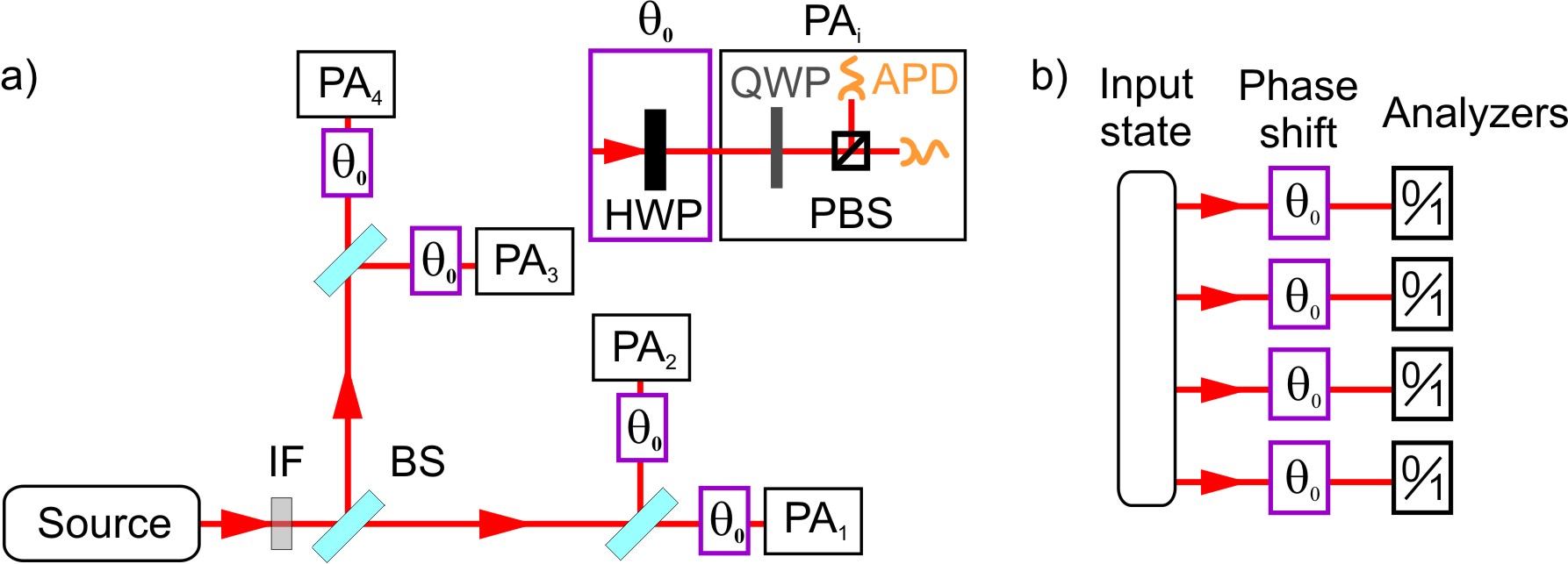
Figure 1: a) Experimental setup. The source uses pulsed parametric down conversion with a type II cut $\beta$-Barium-Borate crystal ($\lambda_{pump}=390$nm) SI . After passing an interference filter (IF), the photons are symmetrically distributed into 4 spatial modes by using 3 non-polarizing beam splitters (BS). The Dicke state $|D_{4}^{(2)}\rangle$ is observed if one photon is detected in each of the four output arms WieczorekPRL09 . The separable state $|\psi_{\rm sep}\rangle$ is created by inserting a $|+\rangle$ polarizer before the first BS. Each polarization qubit is addressed individually and rotated by $\exp[-i\hat{\sigma}_{y}\theta/2]$ (violet box) by a halfwave-plate (HWP). Each polarization analyzer (PA) is composed of a quarterwave-plate (QWP), a polarizing beam-splitter (PBS) and an avalanche photo-diode (APD). b) Schematic of our interferometric setup.

For the experimental demonstration, we use the symmetric four-photon entangled Dicke state KieselPRL07 ; notaFock $|D_{4}^{(2)}\rangle=\big{(}|HHVV\rangle+|HVHV\rangle+|HVVH\rangle+|VHHV\rangle+|VHVH\rangle+|VVHH\rangle\big{)}/\sqrt{6}$ and the separable state $|\psi_{\rm sep}\rangle=|++++\rangle$ observed from multiphoton parametric down conversion WieczorekPRL09 [Fig. 1 a)]. Here $|HHVV\rangle\equiv|H\rangle_{1}\otimes|H\rangle_{2}\otimes|V\rangle_{3}\otimes|V\rangle_{4}$, $|H\rangle_{i}$ ($|V\rangle_{i}$) refer to the horizontal (vertical) polarization of a photon in the spatial mode $i$, and $|\pm\rangle\equiv\frac{1}{\sqrt{2}}(|H\rangle\pm|V\rangle)$. From the measured density matrices ($\rho^{\rm exp}_{D}$ and $\rho^{\rm exp}_{\rm sep}$ SI ) we deduce a fidelity of $0.8872\pm 0.0055$ for $|D_{4}^{(2)}\rangle$ and $0.9859\pm 0.0062$ for $|\psi_{\rm sep}\rangle$ (errors deduced with Poissonian count statistics) and also the QFI determining the suitability of the experimentally observed states for phase estimation. For the ideal Dicke state $|D_{4}^{(2)}\rangle$, the QFI reaches its maximum value, $F_{Q}[|D_{N}^{(N/2)}\rangle,\hat{J}]=N(N+2)/2=12$, when $\hat{\sigma}_{\vec{n}_{i}}=\hat{\sigma}_{y}$ for all $i$ ($\hat{J}\equiv\hat{J}_{y}$) HyllusPRA10 . In the experiment, this choice leads to $F_{Q}[\rho^{\rm exp}_{D},\hat{J}_{y}]=9.999\pm 0.095$, at the maximal value achievable with 3-particle entanglement. An optimization over the local directions ${\vec{n}_{i}}$ HyllusPRA10 , leads to the slightly higher value $F_{Q}^{\rm opt}[\rho^{\rm exp}_{D},\hat{J}^{\rm opt}]=10.326\pm 0.093$, detecting useful 4-particle entanglement with $3.5$ standard deviations. Sure enough, using a witness operator it is possible to prove 4-particle entanglement in a simpler way KieselPRL07 ; SI . With only a subset of the tomographic data we obtain a witness expectation value of $-0.2205\pm 0.0055$, proving 4-particle entanglement with a significance of 40 standard deviations SI . However, witness operators merely recognize entanglement, whereas our criterion directly indicates the state’s applicability for a quantum task. The separable state $|\psi_{\rm sep}\rangle$ ideally allows for sensitivity at the shot-noise limit, $F_{Q}[|\psi_{\rm sep}\rangle,\hat{J}_{y}]=N=4$. The experimental density matrix leads to $F_{Q}[\rho^{\rm exp}_{\rm sep},\hat{J}_{y}]=3.894\pm 0.023$, a value close to the expected separable limit (the optimized value being $F_{Q}^{\rm opt}[\rho^{\rm exp}_{D},\hat{J}^{\rm opt}]=4.014\pm 0.025$).

In order to demonstrate that the precision close to the one predicted by $F_{Q}$ can indeed be achieved in practise, we experimentally implement a phase estimation analysis with the input states $\rho^{\rm exp}_{D}$ and $\rho^{\rm exp}_{\rm sep}$. Our interferometric protocol transforms the probe state by $U(\theta_{0})=\exp[-i\sum_{k=1}^{4}\hat{\sigma}_{\vec{n}_{i}}^{(k)}\theta_{0}/2]$ using the halfwave-plates and phase shifts depicted in Figs 1 a) and b). The unknown value of the phase shift $\theta_{0}$ is inferred from the difference in the number of particles, $2\mu=N_{H}-N_{V}$ ($\mu=-2,-1,0,1,2$), in the states $V$ and $H$. For the ideal states and the rotation directions $\vec{n}_{i}=y$, this measurement is optimal, and hence $F_{\hat{\mu}}=F_{Q}$. Experimentally, the optimized direction and measurement can be different because of noise and misalignment. However, for the observed states the expected improvement would be rather small.

The relation between the phase shift and the possible results of a measurement is provided by the conditional probabilities $P(\mu|\theta_{0})$. These are measured experimentally and compared with the theoretical ones for both the separable and the entangled state, as shown in Fig. 2 a)-k).

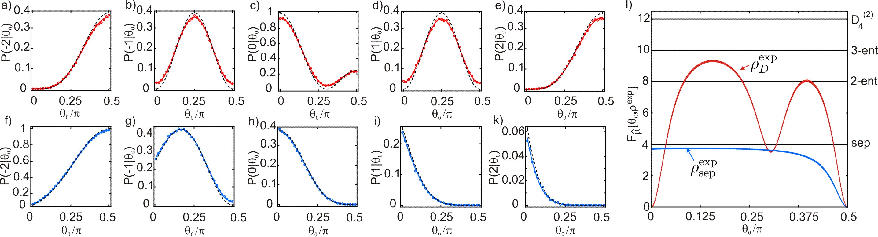
Figure 2: Calibration curves and Fisher information. The small panels show the conditional probabilities $P_{\rm exp}(\mu|\theta_{0})$ for the state $\rho_{D}^{\rm exp}$ [red curve, upper row a)-e)] and for $\rho_{\rm sep}^{\rm exp}$ [blue curve, lower row f)-k)]. Dashed black lines are the ideal probabilities $P(\mu|\theta)$, dots are experimental results. The red and blue curves are fits obtained by assuming that the main source of errors are misalignments in the polarization optics SI . The measurements are performed for 31 values of $\theta_{0}$ by collecting approximately 7000 events for each phase value. Panel l) shows the Fisher information [Eq. (3)], obtained from the fits $P_{\rm exp}(\mu|\theta_{0})$. The line widths correspond to the error intervals $F_{\hat{\mu}}[\theta_{0},\rho^{\rm exp}]\pm\Delta F_{\hat{\mu}}$ with $\Delta F_{\mu}[\rho_{D}^{\rm exp}]\leq 0.08$ and $\Delta F_{\hat{\mu}}[\rho_{\rm sep}^{\rm exp}]\leq 0.04$ SI . Horizontal lines indicate limits for separable states (“sep”, equal to $F_{\hat{\mu}}[|\psi_{\rm sep}\rangle]$), for 2- and 3-particle entangled states, and for the ideal Dicke state $F_{\hat{\mu}}[|\mathrm{D}_{4}^{(2)}\rangle]$. Theoretically, $F_{\hat{\mu}}=F_{Q}$ holds for the ideal input states, phase operations and output measurements. Experimentally, we observe $F_{\hat{\mu}}[\theta_{0},\rho^{\rm exp}]<F_{Q}[\rho^{\rm exp}]$ due to technical noise. In particular, $F_{\hat{\mu}}[\theta_{0},\rho^{\rm exp}_{D}]$ is strongly reduced for values of the phase shift where some of the ideal conditional probability densities $P(\mu|\theta_{0})$ of panels a)-e) go to $0$ ($\theta_{0}=0,0.3\pi,0.5\pi$). For reduced visibilities (when $P_{\rm exp}(\mu|\theta_{0})>0$ while ideally $P(\mu|\theta_{0})=0$), the contribution to the Fisher information is reduced since in these points also the derivatives of $P_{\rm exp}(\mu|\theta_{0})$ vanish, cf. Eq. (3).

A fit to the measured conditional probabilities provides $P_{\rm exp}(\mu|\theta)$, which are used to calculate the Fisher information according to Eq. (3) [see Fig. 2 l)]. As expected, our experimental apparatus can surpass the shot noise limit for a broad range of phase values (where $F_{\hat{\mu}}^{\rm exp}>4$), and can even exploit useful three particle entanglement (where $F_{\hat{\mu}}^{\rm exp}>8$).

The phase shift $\theta_{0}$ is inferred from the results, $\mu_{1},\mu_{2},...,\mu_{m}$, of $m$ independent repetitions of the interferometric protocol. We will refer to such a collection of measurements as a single $m$-experiment. In the experiment, we set the phase shift to 9 known values $\theta_{0}$. For each $\theta_{0}$, 12000 results $\mu_{i}$ are independently measured and grouped into vectors of length $m$ to perform the phase estimation for different values of $m$ $(=1,10,100)$. Using this data, we implement a ML and a Bayesian phase estimation protocol. While both have been recently used in literature for phase estimation KacprowiczNP2010 ; PezzePRL07 , here they are compared in detail and applied for the first time to demonstrate SSN phase uncertainty with more than two particles. To display the quantum enhancement and to compare the methods we use the rescaled uncertainty $\Delta_{\rm res}$ defined below.

In the ML protocol, the estimator $\theta_{\mathrm{est}}$ of the unknown phase shift is determined as the value maximizing the likelihood function ${\cal L}(\theta)=\prod_{i=1}^{m}P_{\rm exp}(\mu_{i}|\theta)$ Cramer_book . For different $m$-experiments it fluctuates with standard deviation $\Delta\theta_{\mathrm{est}}$, which has to be calculated by repeating a large number of single $m$-experiments. For large $m$, the distribution of $\theta_{\mathrm{est}}$ approaches a Gaussian centered on $\theta_{0}$ and of width $\Delta\theta_{\mathrm{est}}$ saturating the CRLB, Eq. (2) Cramer_book .

Fig. 3 shows the distributions of the estimator $\theta_{\mathrm{est}}$ for the phase shift $\theta_{0}=0.2\pi$ and different values of $m$. As expected, with increasing $m$, the histograms approach a Gaussian shape with standard deviation $\Delta\theta_{\mathrm{est}}$ decreasing as $1/\sqrt{mF_{\hat{\mu}}}$. The width of the histograms is smaller for the Dicke state (red lines) than for the separable state (blue lines). Fig. 4 shows $\Delta_{\rm res}=\sqrt{m}\Delta\theta_{\mathrm{est}}$ as a function of $\theta_{0}$. For $m=10$ the standard deviation is below the CRLB (Eq. 2) for several $\theta_{0}$ values. This is possible because the estimation is biased, i.e., for $b\equiv\langle\theta_{\mathrm{est}}\rangle-\theta_{0}$ we have $b\neq 0$ and $\partial_{\theta_{0}}b\neq 0$ Cramer_book ; SI . The bias can be taken into account by replacing the numerator in the CRLB Eq. (2) by $|1-\partial_{\theta_{0}}b|$. For even smaller $m$, only few different maxima of the likelihood functions ${\cal L}(\theta)$ can occur, see Fig. 3 a). Then, $\theta_{\mathrm{est}}$ scatters significantly and hardly allows for an unbiased phase estimate. When $m=100$, the bias is strongly reduced and the agreement of $\Delta\theta_{\mathrm{est}}$ with the unbiased CRLB is improved significantly. While the bias is still large enough to cause apparent sensitivities below the shot-noise limit for the separable state, for the Dicke state the CRLB is saturated for a large phase interval. This clearly proves that the multiparticle entangled Dicke state created experimentally indeed achieves the SSN phase uncertainty predicted by the CRLB Eq. (2) using the experimentally obtained Fisher information from Fig. 2 l).

A conceptually different phase estimation protocol is given by the Bayesian approach assuming that the phase shift is a random variable. The probability density for the true value of the phase shift being equal to $\theta$, conditioned on the measured results $\mu_{1},\mu_{2},...,\mu_{m}$, is provided by Bayes’ theorem, $P(\theta|\{\mu_{i}\}_{i=1}^{m})=P_{\rm exp}(\{\mu_{i}\}_{i=1}^{m}|\theta)P(\theta)/P(\{\mu_{i}\}_{i=1}^{m})$. To define the a priori probability density $P(\theta)$ we adopt the maximum ignorance principle and take $P(\theta)$ to be constant in the phase interval considered. The Bayesian probability density is then given by $P(\theta|\{\mu_{i}\}_{i=1}^{m})\propto\prod_{i=1}^{m}P_{\rm exp}(\mu_{i}|\theta)={\cal L}(\theta)$. The phase shift can be estimated as the maximum of the probability density as before. However, in contrast to the ML method, the Bayesian analysis allows to assign a meaningful uncertainty to this estimate even for a single $m$-experiment and biased estimators. This can be taken, for instance, as a confidence interval $\Delta\theta=C$ around the estimate, where the area of $P(\theta|\{\mu_{i}\}_{i=1}^{m})$ is equal to $68\%$ (see Fig. 3 d) and SI ).

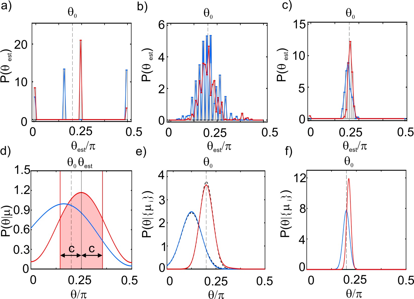
Figure 3: Comparison of the ML method to the Bayesian approach for the estimation of a phase shift $\theta_{0}=0.2\pi$ (vertical dashed black line). Upper row: histograms (normalized to one) of the estimators $\theta_{\mathrm{est}}$ obtained for large number of repetitions of $m$-experiments: a) $m=1$, b) $m=10$, and c) $m=100$. Red (blue) solid lines show the results of the state $\rho_{D}^{\rm exp}$ ($\rho_{\rm sep}^{\rm exp}$). Lower row: exemplary Bayesian probability densities $P(\theta|\{\mu_{i}\}_{i=1}^{m})$ of single $m$-experiments for d) m=1, e) m=10, and f) m=100 for the state $\rho_{D}^{\rm exp}$ (solid red lines) and $\rho^{\rm exp}_{\rm sep}$ (solid blue lines). In panel e) the dashed black lines are Gaussians of width $1/\sqrt{m\,F_{\hat{\mu}}}$ plotted to illustrate that the densities rapidly approach a Gaussian shape. For $m=1$, we plot $P(\theta|\mu=1)$ for $\rho_{D}^{\rm exp}$ and $P(\theta|\mu=-1)$ for $\rho^{\rm exp}_{\rm sep}$. The shaded region indicates the confidence interval $[\theta_{\mathrm{est}}-C,\theta_{\mathrm{est}}+C]$ around the maximum of the distribution.

Figs 3 d)-f) illustrate how the Bayesian probability density evaluated for a single $m$-experiment becomes Gaussian with a width $1/\sqrt{mF_{\hat{\mu}}}$, already for small values of $m$. In contrast, the ML histograms [Figs 3 a)-c)] approach a Gaussian shape more slowly. We also investigated how the Bayesian analysis performs on average using the same data as in the ML case. The results are shown in Fig. 4 with the rescaled Bayesian uncertainty $\Delta_{\rm res}=\sqrt{m}C$ for various $\theta_{0}$ and averaged over several $m$-experiments. For $m=10$ the mean values of the confidences deviate from the CRLB and have a large spread. For $m=100$, however, the confidences agree well with the CRLB for most values of $\theta_{0}$, for both states.

In conclusion, we have investigated experimentally the relation between SSN phase estimation and the entanglement properties of a probe state. We have identified useful multiparticle entanglement by determining the quantum Fisher information from the tomographical data of a four photon Dicke state. The benefit of such entanglement has been demonstrated by implementing two different phase estimation analyses, both of which saturate the Cramer Rao bound and clearly surpass the shot noise limit. The approach is completely general: it applies for any probe state, is scalable in the number of particles and does not require state selection. Our study thus provides a guideline for the future technological exploitation of multiparticle entanglement to outperform current metrological limits.

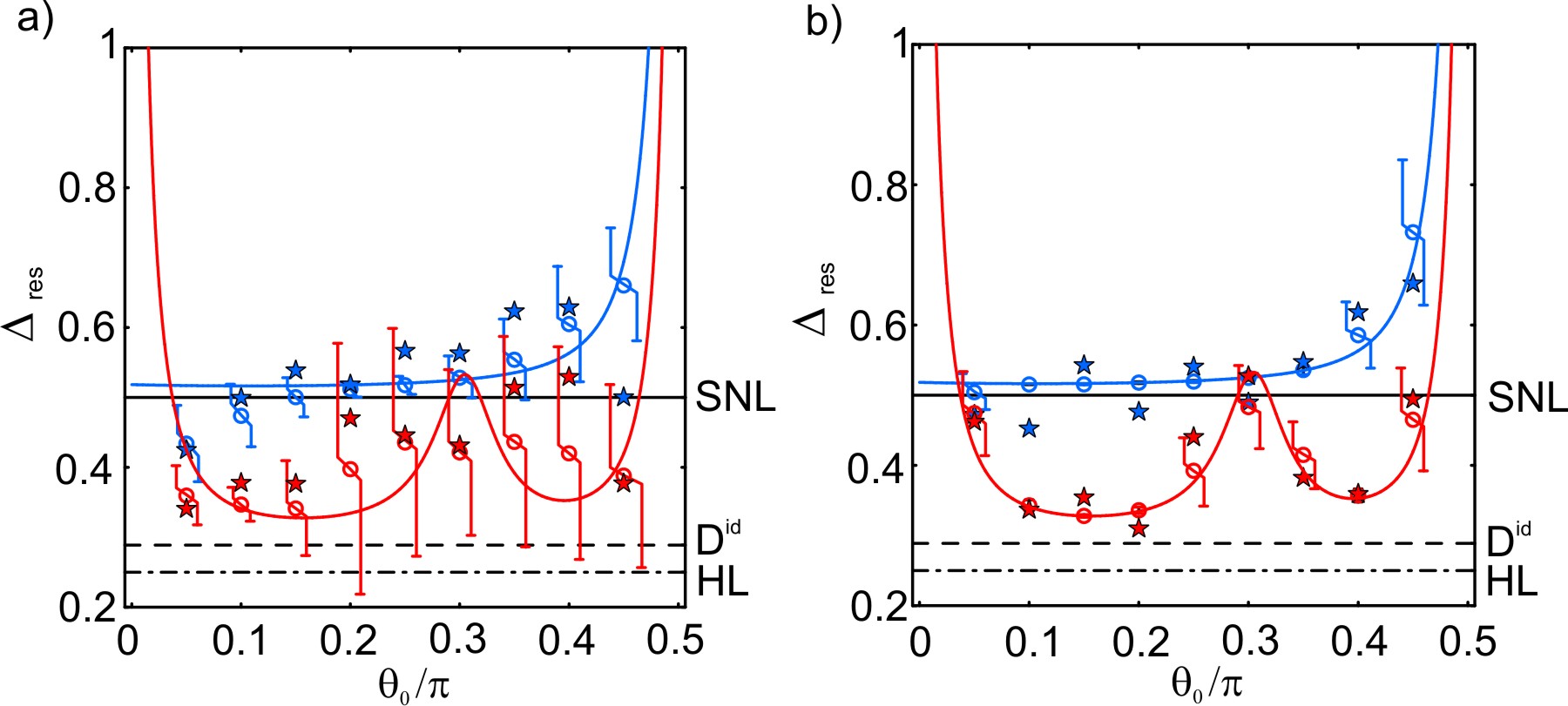
Figure 4: Rescaled phase uncertainties $\Delta_{\rm res}$ obtained with the probe state $\rho^{\rm exp}_{D}$ (red) and $\rho^{\rm exp}_{\rm sep}$ (blue), with a) $m=10$ and b) $m=100$. The solid red (blue) line is the expected uncertainty given by the CRLB [Eq. (2)] using the experimental $F_{\hat{\mu}}$ [see Fig. 2 l)] for the state $\rho^{\rm exp}_{D}$ ($\rho^{\rm exp}_{\rm sep}$). Stars are the results of the ML analysis (standard deviation of $\theta_{\mathrm{est}}$) with $\Delta_{\rm res}=\sqrt{m}\Delta\theta_{\mathrm{est}}$. Circles are the results of the Bayesian analysis with $\Delta_{\rm res}=\sqrt{m}\langle C\rangle$, and the error bars display the scatter of C. Horizontal lines are the shot-noise limit (SNL) (solid line), the limit for an ideal Dicke state ($D^{\rm{id}}$) $\Delta_{\rm res}=1/\sqrt{F_{Q}[|D_{4}^{(2)}\rangle]}$ (dashed line) and the Heisenberg limit (HL) $\Delta_{\rm res}=1/4$ (dot-dashed line).

We thank N. Kiesel, W. Laskowski, and O. Gühne for stimulating discussions. R.K., C.S., W.W., and H.W. acknowledge the support of the DFG-Cluster of Excellence MAP, the EU projects QAP and Q-Essence, and the DAAD/MNISW exchange program. W.W. and C.S. thank QCCC of the Elite Network of Bavaria and P.H. thanks the ERC Starting Grant GEDENTQOPT.

References

(1)
For a recent review see
V. Giovannetti, S. Lloyd, and L. Maccone, Nat. Phot. 5, 222 (2011).
(2)
J.G. Rarity ,
Phys. Rev. Lett. 65, 1348 (1990).
(3) M.W. Mitchell, J.S. Lundeen and A.M. Steinberg,
Nature 429, 161 (2004);
P. Walther ,
429, 158 (2004)
(4) M. Kacprowicz ,
Nature Phot. 4 357 (2010).
(5) T. Nagata, ,
Science 316, 726 (2007).
(6) Xiang, G. Y., et al.,Nature Phot.5 43 (2010).
(7) J. Appel ,
PNAS 106, 10960 (2009);
M. H. Schleier-Smith ,
Phys. Rev. Lett. 104 073604 (2010).
(8) D. Leibfried ,
Science 304, 1476 (2004).
(9) C. Gross ,
Nature 464, 1165 (2010).
(10) M. F. Riedel ,
Nature 464, 1170 (2010).
(11)
K.J. Resch ,
Phys. Rev. Lett. 98, 223601 (2007).
(12)L. Pezzé and A. Smerzi,
Phys. Rev. Lett. 102, 100401 (2009).
(13)
P. Hyllus ,
http://arxiv.org/abs/1006.4366;
G. Tóth,
http://arxiv.org/abs/1006.4368.
(14) C.W. Helstrom,
Phys. Lett. 25A, 101 (1967);
S.L. Braunstein and C.M. Caves,
Phys. Rev. Lett. 72 3439 (1994).
(15)
See supplementary material for additional information.
(16) A pure state is called -particle entangled
if ,
where is a non-factorizable state of
particles, and for at least one SI .
(17)
D.M. Greenberger, M.A. Horne and A. Zeilinger, Going beyond Bell’s theorem
(Kluwer Academics, 1989).
(18) V. Giovannetti, S. Lloyd and L. Maccone,
Phys. Rev. Lett. 96, 010401 (2006).
(19) H. Cramér, Mathematical Methods of Statistics
(Princeton Univ. Press, 1946).
(20)
Note that it is possible to further improve the
sensitivity by applying the phase shift several
times to the probe system
GiovannettiPRL06 .
(21)
N. Kiesel ,
Phys. Rev. Lett. 98, 063604 (2007).
(22) For indistinguishable qubits
the symmetric Dicke state reduces to a Twin-Fock state, see
M.J. Holland and K. Burnett,
Phys. Rev. Lett. 71 1355 (1993).
(23)
W. Wieczorek ,
Phys. Rev. Lett. 103, 020504 (2009).
(24) P. Hyllus, O. Gühne and A. Smerzi,
Phys. Rev. A 82, 012337 (2010).
(25)L. Pezzé ,
Phys. Rev. Lett. 99, 223602 (2007);
Z. Hradil ,
Phys. Rev. Lett. 76, 4295 (1996).