Intrinsic filtering errors of Lagrangian particle tracking
in LES flow fields

Abstract

Large-Eddy Simulations (LES) of two-phase turbulent flows exhibit quantitative differences in particle statistics if compared to Direct Numerical Simulations (DNS) which, in the context of the present study, is considered the exact reference case. Differences are primarily due to filtering, a fundamental intrinsic feature of LES. Filtering the fluid velocity field yields approximate computation of the forces acting on particles and, in turn, trajectories that are inaccurate when compared to those of DNS. In this paper, we focus precisely on the filtering error for which we quantify a lower bound. To this aim, we use a DNS database of inertial particle dispersion in turbulent channel flow and we perform a-priori tests in which the error purely due to filtering is singled out removing error accumulation effects, which would otherwise lead to progressive divergence between DNS and LES particle trajectories. By applying filters of different type and width at varying particle inertia, we characterize the statistical properties of the filtering error as a function of the wall distance. Results show that filtering error is stochastic and has a non-Gaussian distribution. In addition, the distribution of the filtering error depends strongly on the wall-normal coordinate being maximum in the buffer region. Our findings provide insight on the effect of subgrid-scale velocity field on the force driving the particles, and establish the requirements which a LES model must satisfy to predict correctly the velocity and the trajectory of inertial particles.

I Introduction

The dispersion of small inertial particles in inhomogeneous turbulent flow has been long recognized as crucial in a number of industrial applications and environmental phenomena. Examples include mixing, combustion, depulveration, spray dynamics, pollutant dispersion or cloud dynamics. In all these problems accurate predictions are important, yet not trivial to obtain because of the complex phenomenology that controls turbulent particle dynamics.

Direct Numerical Simulations (DNS) of turbulence coupled with Lagrangian Particle Tracking (LPT) hit2 ; ms02 ; hit1 ; fs06 ; re01 ; Soldati2009 ; mgss03 ; uo96 have demonstrated their capability to capture the physics of particle dynamics in relation with turbulence dynamics and have highlighted the key role played by inertial clustering and preferential concentration in determining the rates of particle interaction, settling, deposition and entrainment. Due to the computational requirements of DNS, however, analysis of applied problems characterized by complex geometries and high Reynolds numbers demands alternative approaches, among which Large-Eddy Simulation (LES) is gaining in popularity, especially for cases where the large flow scales control particle motion (e.g. apte ; okong ).

LES is based on a filtering approach in which the unresolved Sub-Grid Scales (SGS) of turbulence are modeled. A major issue associated with LES of particle-laden flows is modeling the effect of these scales on particle dynamics. Flow anisotropy adds a further complicacy. In particular, recent studies on particle dispersion in wall-bounded turbulence kv05 ; k06 ; Marchioli2008 ; Khan2010 have demonstrated that use of the filtered fluid velocity in the equation of particle motion with no model for the effect of the SGS fluid velocity fluctuations leads to significant underestimation of preferential concentration and, consequently, to weaker deposition fluxes and lower near-wall accumulation. Even though several studies have demonstrated that predictions may be improved using techniques like filter inversion or approximate deconvolution kv05 ; k06 ; sm05 ; Gobert2010 ; Marchioli2008b , the amount of velocity fluctuations that can be reintroduced in the particle equations does not ensure a quantitative replica of DNS results. A further effort is required to model the scales smaller than the filter width but extremely significant for particle dynamics, which are inevitably lost in the filtering procedure Marchioli2008b . Attempts to model SGS effects on particles have been made using fractal interpolation Marchioli2008b or kinematic simulations Khan2010 in channel flow. Also these approaches, however, do not ensure complete removal of inaccuracies in the quantitative prediction of local particle segregation and accumulation (particularly in the near-wall region). Stochastic models have also been proposed, yet we are only aware of validations in homogeneous isotropic turbulence sm06 ; Pozorski2009 ; Gobert2010 : these models have still to be assessed in non-homogeneous anisotropic flows.

To devise accurate and reliable SGS models for LPT, precise quantification of filtering effects on particle dynamics is clearly a necessary step. Aim of this paper is to propose a simple procedure to characterize the subgrid error kv05 purely due to filtering of the fluid velocity field. This error, referred to as pure filtering error hereinafter, can not be avoided but potentially can be corrected. We thus focus on an ideal situation in which LES provides the exact dynamics of the resolved velocity field (ideal LES). In ideal LES, modeling and numerical errors (incurred because a real LES provides only an approximation of the filtered velocity) and interpolation errors (on coarse-grained domains, for instance) kv05 are assumed negligible, and a lower bound for the pure filtering error can be identified. Peculiar feature of the procedure proposed here is that it removes time accumulation of pure filtering errors on particle trajectories. Error accumulation originates from inaccurate estimation of the forces acting on particles obtained when the filtered fluid velocity is supplied to the equation of particle motion. As a result, particle trajectories in LES fields progressively diverge from particle trajectories in DNS fields, considered as the exact reference for the present study: the flow fields seen by the particles become less and less correlated and the forces acting on particles are evaluated at increasingly different locations. We remark that the effects due to these two errors can not be singled out easily when comparing statistics of particle velocity and concentration obtained from LES to the reference DNS data. To remove this effect, we perform here a-priori tests in which: (i) particle trajectories are computed from the DNS fields, (ii) the DNS fields are coarse-grained through filtering and, (iii) particles are forced to evolve in the filtered DNS fields along the DNS trajectories. A similar a-priori analysis has been performed recently to evaluate pure filtering error and time accumulation error for the case of tracer particle dispersion in homogeneous isotropic turbulence Calzavarini2010 . In this paper, we focus on inertial particles in turbulent channel flow.

A-priori evaluation of the statistical properties of the filtering error provides useful information about the key features that should be incorporated in SGS models for LPT to compensate for such error. Statistics are computed applying filters of different type and different widths, corresponding roughly to varying amounts of resolved flow energy, and considering point particles with different inertia that obey one-way coupled Stokes dynamics. One point at issue is indeed whether SGS models for LPT should take into account inertial effects explicitly. Another point to be explored is whether the characteristics of SGS models for LPT should adapt “dynamically” to respond to the local inhomogeneity and anisotropy of the flow. Our study aims at addressing these issues through statistical characterization of the effects of the unresolved velocity field on the force driving the particles. Possible ways to improve prediction of LES applied to turbulent dispersed flow should be benchmarked against this type of statistical information at the sub-grid level.

The paper is organized as follows. The physical problem and the numerical methodology are described in Sec. II. The statistical moments and the probability distribution functions of the filtering error are presented in Sec. III and in Sec. IV, respectively. Finally, concluding remarks are given in Sec. V.

II Physical Problem and Numerical Methodology

II.1 Particle-laden turbulent channel flow

The reference flow configuration consists of two infinite flat parallel walls: the origin of the coordinate system is located at the center of the channel and the $x-$, $y-$ and $z-$ axes point in the streamwise, spanwise and wall-normal directions respectively. Periodic boundary conditions are imposed on the fluid velocity field in $x$ and $y$, no-slip boundary conditions are imposed at the walls. In the present study, we consider air (assumed to be incompressible and Newtonian) with density $\rho=1.3~{}kg~{}m^{-3}$ and kinematic viscosity $\nu=15.7{\times}10^{-6}~{}m^{2}~{}s^{-1}$. The flow is driven by a mean pressure gradient, and the shear Reynolds number is $Re_{\tau}=u_{\tau}h/\nu=150$, based on the shear (or friction) velocity, $u_{\tau}$, and on the half channel height, $h$. The shear velocity is defined as $u_{\tau}=(\tau_{w}/\rho)^{1/2}$, where $\tau_{w}$ is the mean shear stress at the wall.

Particles are modeled as pointwise, non-rotating rigid spheres with density $\rho_{p}=10^{3}~{}kg~{}m^{-3}$, and are injected into the flow at concentration low enough to consider dilute system conditions (no inter-particle collisions) and one-way coupling between the two phases (no turbulence modulation by particles). The motion of particles is described by a set of ordinary differential equations for particle velocity and position. For particles much heavier than the fluid ($\rho_{p}/\rho\gg 1$) Elghobashi and Truesdell et92 have shown that the most significant forces are Stokes drag and buoyancy and that Basset force can be neglected being an order of magnitude smaller. In the present simulations, the aim is to minimize the number of degrees of freedom by keeping the simulation setting as simplified as possible; thus the effect of gravity has also been neglected. With these assumptions, a simplified version of the Basset-Bousinnesq-Oseen equation Gatignol is obtained. In vector form:

$$\frac{d{\bf x}_{p}}{dt}={\bf v}_{p}~{},$$ (1)

$$\frac{d{\bf v}_{p}}{dt}=\frac{\mathbf{u}_{s}-\mathbf{v}_{p}}{\tau_{p}}(1+0.15Re_{p}^{0.687})~{}.$$ (2)

In Eqns. (1) and (2), ${\bf x}_{p}$ is particle position, ${\bf v}_{p}$ is particle velocity, ${\bf u}_{s}={\bf u}({\bf x}_{p}(t),t)$ is the fluid velocity at the particle position. $\tau_{p}=\rho_{p}d^{2}_{p}/18\mu$ is the particle relaxation time, and $Re_{p}=d_{p}|{\bf v}_{p}-{\bf u}_{s}|\rho/\mu$ is the particle Reynolds number, $d_{p}$ and $\mu$ being the particle diameter and the fluid dynamic viscosity respectively.

II.2 DNS/LPT methodology

The Eulerian flow field is obtained using a pseudo-spectral DNS flow solver which discretizes the governing equations (Continuity and Navier-Stokes for incompressible flow) by transforming the field variables into wavenumber space, using Fourier representations for the periodic streamwise and spanwise directions and a Chebyshev representation for the wall-normal (non-homogeneous) direction. A two level, explicit Adams-Bashforth scheme for the non-linear terms, and an implicit Crank-Nicolson method for the viscous terms are employed for time advancement. Further details of the method can be found in previous articles (e.g. Pan and BanerjeePB_POF_96 ). Calculations were performed on a computational domain of size $L_{x}\times L_{y}\times L_{z}=4\pi h\times 2\pi h\times 2h$ in $x$, $y$ and $z$ respectively, corresponding to $1885\times 942\times 300$ in wall units. Wall units are obtained combining $u_{\tau}$, $\nu$ and $\rho$. The computational domain is discretized in physical space with $N_{x}\times N_{y}\times N_{z}=128\times 128\times 129$ grid points (corresponding to $128\times 128$ Fourier modes and to 129 Chebyshev coefficients in the wavenumber space). This is the minimum number of grid points required in each direction to ensure that the grid spacing is always smaller than the smallest flow scale and that the limitations imposed by the point-particle approach are satisfied. Marchioli2008

To calculate particle trajectories a Lagrangian tracking routine is coupled to the flow solver. The routine solves for Eqns. (1) and (2) using a $4^{th}$-order Runge-Kutta scheme for time advancement and $6^{th}$-order Lagrangian polynomials for fluid velocity interpolation at the particle location. At the beginning of the simulation, particles are distributed randomly within the computational domain and their initial velocity is set equal to that of the fluid at the particle initial position. Periodic boundary conditions are imposed on particles moving outside the computational domain in the homogeneous directions, perfectly-elastic collisions at the smooth walls are assumed when the particle center is at a distance lower than one particle radius from the wall. For the simulations presented here, large samples of $10^{5}$ particles, characterized by different response times, are considered. When the particle response time is made dimensionless using wall variables, the Stokes number for each particle set is obtained as $St=\tau_{p}/\tau_{f}$ where $\tau_{f}=\nu/u_{\tau}^{2}$ is the viscous timescale of the flow. Three different sets of particles corresponding to values of the Stokes number $St=1$, $5$ and $25$ have been considered in this study: Table 1 shows the relevant physical parameters of each set. The total tracking time in dimensionless wall units (identified hereinafter by superscript +) is $\Delta T^{+}=21150$ for all particle sets Marchioli2008 , the timestep size for particle tracking being equal to the timestep size used for the fluid: $\delta t^{+}=0.045$.

II.3 A-priori LES methodology and computation of the filtering error

In the a-priori tests, LPT is carried out replacing ${\bf u}_{s}$ in Eq. (2) with the filtered fluid velocity field, $\bar{{\bf u}}({\bf x_{p}},t)$. This field is obtained through explicit filtering of the DNS velocity by either a cut-off filter or a top-hat filter. Both filters are applied in the wave number space to velocity components in the homogeneous streamwise and spanwise directions:

$$\bar{u}_{i}({\bf x},t)=FT^{-1}\left\{\begin{array}[]{ll}{\hat{G}}(\kappa_{1})\cdot{\hat{G}}(\kappa_{2})\cdot\hat{u}_{i}(\kappa_{1},\kappa_{2},z,t)~{}~{}{{\text{if}}~{}|\kappa_{j}|\leq|\kappa_{c}|~{}{\text{with}}~{}j=1,2}\\ 0\hskip 142.26378pt\text{otherwise}\end{array}\right.$$ (5)

where $FT$ is the 2D Fourier Transform, $\kappa_{c}=\pi/\Delta$ is the cutoff wave number ($\Delta$ being the filter width in the physical space), $\hat{u}_{i}(\kappa_{1},\kappa_{2},z,t)$ is the Fourier transform of the DNS fluid velocity field, namely $\hat{u}_{i}(\kappa_{1},\kappa_{2},z,t)=FT[{u}_{i}({\bf x},t)]$ and ${\hat{G}}(\kappa_{j})$ is the filter transfer function:

$$G(\kappa_{j})=\left\{\begin{array}[]{ll}1~{}~{}~{}~{}~{}~{}~{}~{}~{}~{}~{}~{}~{}~{}~{}~{}~{}~{}~{}{\text{for the cut-off filter}}\\ \frac{sin(\kappa_{j}\Delta/2)}{\kappa_{j}\Delta/2}~{}~{}~{}~{}~{}~{}~{}~{}~{}\text{for the top-hat filter}\end{array}\right.$$ (8)

Three different filter widths are considered, which provide a grid Coarsening Factor (CF) in each homogeneous direction of 2, 4 and 8 with respect to DNS, corresponding to $64\times 64$, $32\times 32$ and $16\times 16$ Fourier modes respectively. Note that CF=2 and CF=4 yield grid resolutions that are commonly used in LES, whereas CF=8 corresponds to a very coarse resolution characteristic of under-resolved LES. Data are not filtered in the wall-normal direction, since the wall-normal resolution in LES is often DNS-like. pope-faq

The pure filtering error is computed under the ideal assumption that all further sources of error affecting particle tracking in LES can be disregarded and that the exact dynamics of the resolved velocity field are available. Errors due to the SGS model for the fluid and to numerics are thus neglected and a lower bound for the filtering error is identified by removing error accumulation effects due to progressive divergence between DNS and LES particle trajectories. Time accumulation of the pure filtering error is prevented by computing particle trajectories in DNS fields and then forcing particles to evolve in filtered DNS fields along the DNS trajectories. At each time step $n$ and for each particle $k$ we thus impose:

$$\mathbf{x}_{p,k}^{LES}(t^{n})=\mathbf{x}_{p,k}^{DNS}(t^{n})\equiv\mathbf{x}_{p,k}(t^{n})\;\;;\;\;\mathbf{v}_{p,k}^{LES}(t^{n})=\mathbf{v}_{p,k}^{DNS}(t^{n})\equiv\mathbf{v}_{p,k}(t^{n})~{}~{},$$ (9)

where superscripts $LES$ and $DNS$ identify particle position and velocity in a-priori LES and in DNS, respectively. The pure filtering error made on the $k$-th particle at time $t^{n}$ is computed as:

$$\mathbf{\delta u}\equiv\mathbf{\delta u}(\mathbf{x}_{p,k}(t^{n}),t^{n})=\mathbf{u}(\mathbf{x}_{p,k}(t^{n}),t^{n})-\bar{\mathbf{u}}(\mathbf{x}_{p,k}(t^{n}),t^{n})\equiv\mathbf{u}_{s}-\bar{\mathbf{u}}_{s}~{}~{}.$$ (10)

Due to the wall-normal dependence of the fluid velocity (and of $\mathbf{u}_{s}$ in particular), it is not straightforward to select a characteristic velocity to normalize $\delta{\bf u}$. We thus decided to provide measures of the absolute filtering error rather than the percent filtering error, using Eq. (10) to quantify exactly the filtering error affecting the fluid velocity seen by the particles. This quantification relies on an idealized situation which serves the purpose of isolating the contribution due to filtering of the velocity field to the total error associated with LPT in LES. Note also that $\mathbf{\delta u}$ is computed along the “exact” trajectory of each particle, that is at ${\bf x}_{p,k}^{DNS}(t^{n})$. As shown in the following, the corresponding behavior observed for $\mathbf{\delta u}$ may be significantly different from the Eulerian measure of the filtering error usually found in the literature, which is obtained as difference between DNS and LES velocities at fixed points in space.

Computation and statistical characterization of $\mathbf{\delta u}$ were carried out for all particle sets reported in Table 1 and applying filters of different type and width. The averaging time window required for converged statistics was $\Delta t^{+}\simeq 8285$.

III Statistical moments of the pure filtering error

The Eulerian statistical moments of the filtering error, quantified here by its lower bound $\mathbf{\delta u}$ (Eq. (10)), are presented and analyzed in this section. Statistics were computed by dividing the computational domain in wall-parallel slabs having dimensions $L_{x}$, $L_{y}$ and $\Delta_{z}(i)$ with $i=1,N_{z}$, where $\Delta_{z}(i)$ is the difference between two adjacent Chebyshev collocation points. Ensemble averaging is carried out over particles that, at a given time instant, are located inside the same slab; time averaging is performed over the time interval $\Delta t^{+}$. All quantities shown in this section are non dimensional and expressed in wall units.

III.1 Influence of particle inertia on the filtering error

To analyze the effect of particle inertia on the behavior of $\delta{\bf u}$, we compare statistics relative to all particle sets but we focus one filter type (cut-off) and one filter width (CF=4). This filter width is chosen as it removes a significant amount of spatial information on the turbulent structures which interact with particles without generating overly under-resolved fields. The effects due to different filter types and widths will be investigated in Sec. III.2.

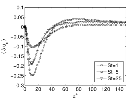
(a)
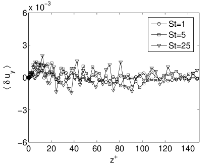
(b)
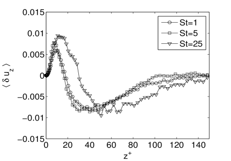
(c)

Figure 1: Mean values of the filtering error $\delta{\bf u}$ in the streamwise (a), spanwise (b) and wall-normal (c) directions as a function of $z^{+}$ at varying particle inertia. Profiles refer to the cut-off filter with CF=4.

Figure 1 shows the mean absolute value $\langle\delta{\bf u}\rangle$ of the filtering error along the streamwise, spanwise and normal directions as a function of the distance from the wall. Hereinafter $\langle\cdot\rangle$ identifies time- and ensemble-averaged quantities. The qualitative behavior of the streamwise component $\langle\delta u_{x}\rangle$ (Fig. 1a) is similar for all particle sets: profiles appear rather flat in the central region of the channel ($60<z^{+}<150$) where $\langle\delta u_{x}\rangle$ is nearly zero and develop a peak in the near-wall region where $\langle\delta u_{x}\rangle$ becomes more and more negative as the wall is approached. Negative $\langle\delta u_{x}\rangle$ means over-estimation of the streamwise drag acting on the particles due to filtering. Maximum overestimation occurs at $z^{+}\simeq 15-20$: the location of this maximum does not change for different inertia. Inertia has a strong effect on the magnitude of the peak, which is maximum for $St=5$ and falls off on either side of this value. This non-monotonic dependence can be explained considering that inertial particles are low-pass filters that respond selectively to removal of sub-grid flow scales according to a characteristic frequency proportional to $1/\tau_{p}$ Marchioli2008 . When the frequency of the removed scales is equal to the characteristic frequency of the particles, particle response is maximized. This is precisely the case of Fig. 1a), in which filtering with CF=4 are observed to produce larger errors for the $St=5$ particles compared to the other particle sets. We remark that inertia also plays a role in transferring filtering errors on fluid velocity into filtering errors on drag, which are proportional to $\langle\delta{\bf u}\rangle\cdot St$.

Filtering has no significant effect in mean on the spanwise component $\langle\delta u_{y}\rangle$ (Fig. 1b) which is characterized by very small values $-$${\cal O}(10^{-3})$ $-$oscillating around zero along the entire channel height. In the spanwise direction, however, both $\langle{\bar{u}}_{s}\rangle$ and $\langle u_{s}\rangle$ attain negligible values. More interesting observations can be drawn examining the wall-normal component, $\langle\delta u_{z}\rangle$ (Fig. 1c). First, we notice that $\langle\delta u_{z}\rangle$ profiles develop a positive peak in the near-wall region which increases in magnitude with the Stokes number. Moving away from this region, values become negative and then relax to zero toward the center of the channel. This means that drag may be either underestimated or overestimated depending on the particle-to-wall distance, a feature not trivial to be reproduced in a model. The observed behavior of $\langle\delta u_{z}\rangle$ also shows that filtering in the homogeneous directions has consequences on the unfiltered inhomogeneous direction. The filtering error propagates in the wall-normal direction according to the relation $\bar{u}_{z}({\bf x},t)=FT^{-1}\left[{\hat{G}}(\kappa_{1})\cdot{\hat{G}}(\kappa_{2})\cdot\hat{u}_{z}(\kappa_{1},\kappa_{2},z,t)\right]$, see Eq. (5).

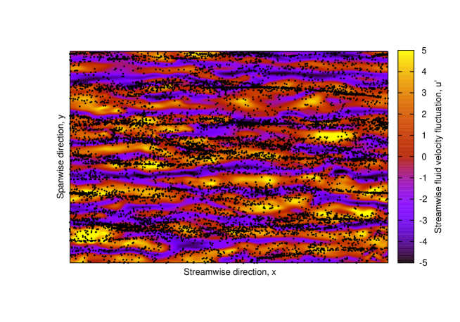
(a)

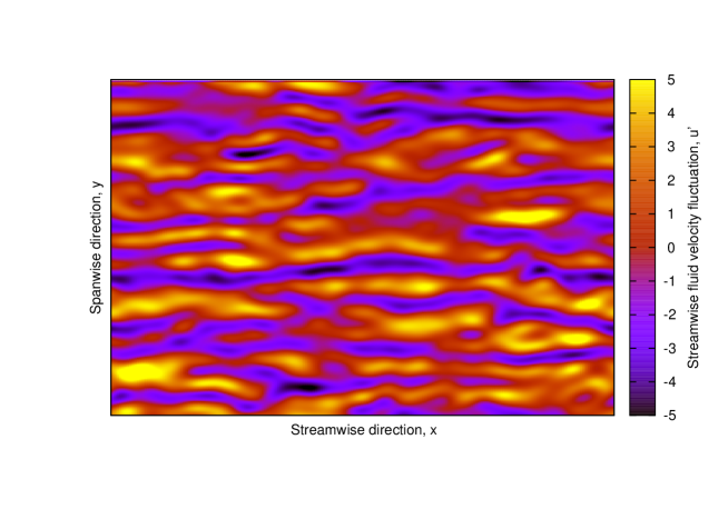
(b)

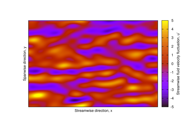
(c)

Figure 2: Fluid streaks in the near-wall region. Low-speed (resp. high-speed) streaks are rendered using colored contours of negative (resp. positive) streamwise fluctuating velocity $u_{x}^{\prime}$ on a horizontal plane at $z^{+}=10$ from the wall. Panel (a) shows the streaky structures obtained from DNS; the instantaneous distribution of the $St=25$ particles comprised between $z^{+}=10$ and the wall is also shown to highlight preferential distribution into the low-speed streaks. Panels (b) and (c) show the streaky structures obtained from a-priori DNS with coarsening-factor 4 and 8, respectively.

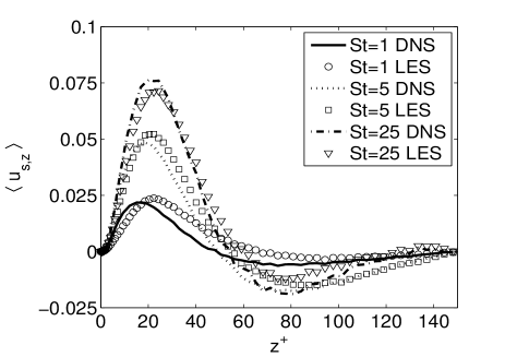
Figure 3: Effects of filtering on the mean wall-normal fluid velocity seen by the particles at varying particle inertia. Profiles refer to the cut-off filter with CF=4.

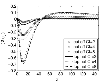
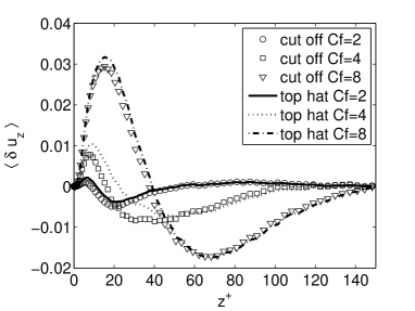
(a)	(b)

Figure 6: Mean values of the filtering error $\delta{\bf u}$ in the streamwise (a), and wall-normal (b) directions as a function of $z^{+}$ at varying filter type and width. Profiles refer to the $St=5$ particles.

We remark that all components of $\delta{\bf u}$ would be rigorously equal to zero if computed at fixed grid points rather than along particle trajectories. This because filtering does not affect the mean value of the velocity. In a-priori and a-posteriori tests, it is customary to analyze the effects of filtering on the LES fluid velocity fields at fixed points (see e.g. kv05 ; Marchioli2008 ). When dealing with LPT, however, a more natural approach is to evaluate filtering effects on the fluid velocity seen by the particles: in this way, both filtering effects on turbulent structures and preferential concentration effects are reproduced in the behavior of $\mathbf{\delta u}$. From a physical viewpoint, this establishes a direct link between $\mathbf{\delta u}$ and the phenomenology of particle dispersion in turbulent boundary layer. To elaborate, it is well known that near-wall turbulence is characterized by the presence of low-speed and high-speed streaks and that inertial particles preferentially sample low-speed streaks Picciotto2005 ; Picciotto2005b ; Soldati2009 . Visual evidence of this tendency is provided in Fig. 2a, in which the instantaneous position of the $St=25$ particles comprised within a near-wall region $10$ wall units thick is superposed to fluid streaks on a ($x;y$)-plane close to the wall ($z^{+}=10$). Fluid streaks are rendered using colored contours of the streamwise fluid velocity fluctuation $u_{x}^{\prime}$ in a DNS flow field. The effect of filtering becomes clear upon comparison of Fig. 2a with Figs. 2b-2c, which demonstrate how rendering of the streaky structures deteriorates when using a coarse-grained flow field (with coarsening factors 4 and 8, in this specific case). Filtering attenuates the velocity fluctuations and smooths the streaks thus increasing the fluid velocity seen by the particles: this is precisely what causes the negative peaks of $\langle\delta u_{x}\rangle$ in Fig. 1a. The behavior of $\langle\delta u_{z}\rangle$ can also be explained in terms of filtering effects on the wall-normal fluid velocity seen by the particles, shown in Fig. 3 for all particle sets. Lines refer to DNS profiles ($\langle u_{s,z}\rangle$), symbols to a-priori LES profiles ($\langle\bar{u}_{s,z}\rangle$). Note that $\langle\delta u_{z}\rangle=\langle u_{s,z}-\bar{u}_{s,z}\rangle=\langle u_{s,z}\rangle-\langle\bar{u}_{s,z}\rangle$. Even though particles exhibit a mean wallward drift, both $\langle u_{s,z}\rangle$ and $\langle\bar{u}_{s,z}\rangle$ are positive (namely directed away from the wall) in the near-wall region due to particle preferential concentration in ejection-like environments, where low-momentum fluid is entrained off the wall Picciotto2005 . Filtering reduces the wall-normal fluid velocity seen by the particles very close to the wall while increasing it towards the center of the channel. This is due to smoothing of the near-wall structures and attenuation of the sweep events, which are characterized by coherent motions of high-momentum fluid to the wall (see e.g. Fig. 6 in Marchioli et al.Marchioli2011 ).

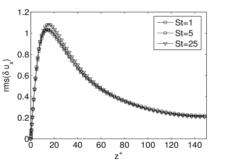
(a)

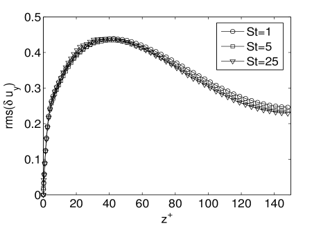
(b)

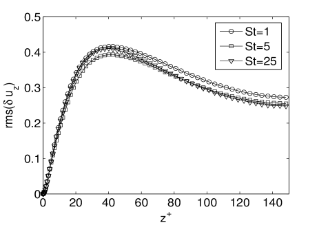
(c)

Figure 4: Rms of the filtering error $\delta{\bf u}$ in the streamwise (a), spanwise (b) and wall-normal (c) directions as a function of $z^{+}$ at varying particle inertia. Profiles refer to the cut-off filter with CF=4.

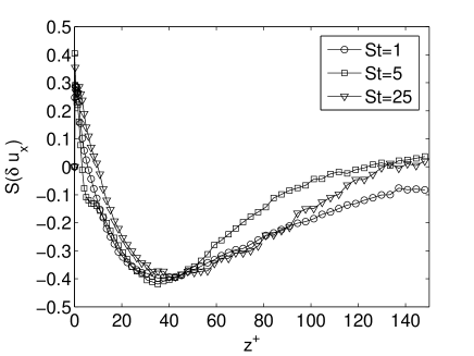
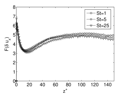
(a)                                                                       (b)

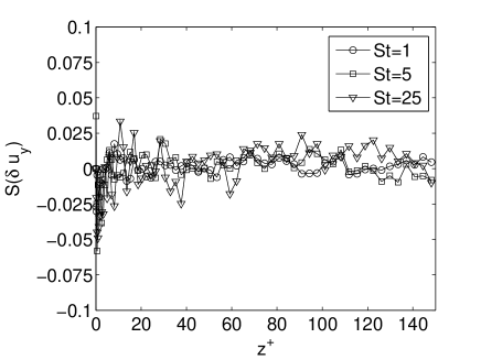
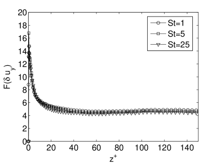
(c)                                                                       (d)

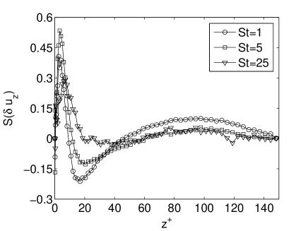
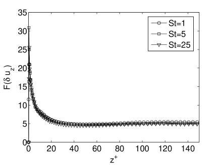
(e)                                                                       (f)

Figure 5: Skewness and flatness of the filtering error $\delta{\bf u}$ in the streamwise (a-b), spanwise (c-d) and wall-normal (e-f) directions as a function of $z^{+}$ at varying particle inertia. Profiles refer to the cut-off filter with CF=4.

Examination of $\langle\delta{\bf u}\rangle$ confirms that LES is inaccurate in capturing the near-wall turbulent structures and in reproducing quantitatively their interaction with particles. Errors introduced by filtering lead to underestimation of preferential concentration and wall accumulation, as demonstrated by previous studies kv05 ; k06 ; Marchioli2008 . To provide a thorough characterization of these errors, in Figs. 4 and 5 we examine the higher order moments. Analysis of the root mean square (rms) of the filtering error, shown in Fig. 4, highlights the reduction of the fluid velocity fluctuations in LES already found in error analyses carried out at fixed (Eulerian) points kv05 . SGS models previously used for LPT in LES fields, like approximate deconvolution or filtering inversion, are mainly aimed at counteracting this effect by recovering the correct amount of fluid and particle velocity fluctuations in the particle equations k06 ; Marchioli2008 . Note that, except in the very-near wall region, rms values of the error are in general much higher than the mean values along the same flow direction: only in the streamwise direction and within the buffer layer, $rms(u_{x})$ and $\langle\delta u_{x}\rangle$ have the same order of magnitude. No significant effects due to particle inertia are observed.

The skewness and flatness factors of the filtering error in each flow direction are shown in Fig. 5, indicated as $S(\mathbf{\delta u})$ and $F(\mathbf{\delta u})$ respectively. As for the rms, the most interesting results are obtained for the skewness in the streamwise and wall-normal directions ($S(\delta u_{x})$ and $S(\delta u_{z})$ in Figs. 5a and 5e, respectively): values of the skewness in the spanwise direction ($S(\delta u_{y})$ in Figs. 5c remain very small along the entire channel height, roughly oscillating around zero. Qualitatively, the skewness profiles in the streamwise and wall-normal directions are similar: moving from the wall toward the center of the channel, both $S(\delta u_{x})$ and $S(\delta u_{z})$ exhibit high positive values in the viscous sublayer followed by low negative values in the buffer region which then relax toward zero at the channel centerline. This behavior indicates that significant asymmetric deviations from Gaussianity are expected in the probability distribution functions of the streamwise and wall-normal components of the filtering error due to significant contributions given by strong isolated events. This finding is consistent with previous analyses kv05 ; Marchioli2008 which showed that filtering impacts particle dynamics mainly through attenuation of low-speed streaks (negative velocity fluctuations) and ejection events. Regarding inertial effects, changes in the Stokes number modify the $S(\delta u_{x})$ profiles particularly in the central portion of the channel, while larger deviations among the $S(\delta u_{z})$ profiles are observed in the near-wall region. Inertia has almost no effect on the flatness factors, shown in Figs. 5b, 5d), and 5f: all profiles are characterized by high values at the wall which gradually decrease to centerline values of about 5 for $F(\delta u_{x})$ and $F(\delta u_{z})$ and of about 4 for $F(\delta u_{y})$. Note that these values are higher than 3, which would be obtained if the error distribution was Gaussian.

III.2 Influence of filter type and width on the filtering error

To investigate the effect of filter type and width on the statistical moments of $\delta{\bf u}$, we focus on the $St=5$ particles. Filter effects on the mean value of the filtering error $\langle\delta{\bf u}\rangle$ are shown in Fig. 6. The streamwise component ($\langle\delta u_{x}\rangle$, Fig. 6a), exhibits a near-wall negative peak whose absolute value increases with the filter width, namely with CF. This behavior is common to all particle sets investigated in this study. Regarding the filter type, it is observed that the top-hat filter introduces a slightly stronger smoothing of the fluid velocity fluctuations compared to the cut-off filter, especially for CF=2 and CF=4, The mean spanwise component of $\langle\delta{\bf u}\rangle$ is not shown since it is characterized by values that are nearly zero throughout the channel. The wall-normal component $\langle\delta u_{z}\rangle$ is shown in Figure 6b. It is evident that the behavior of $\langle\delta u_{z}\rangle$ is influenced significantly by the filter width rather than by the filter type. As CF increases, the profiles develop positive and negative peaks of different intensity; also the distance from the wall at which these peaks occur changes considerably: all peak locations shift toward the center of the channel, indicating that filtering errors propagate their effect over a larger portion of the computational domain.

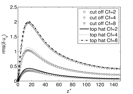
(a)

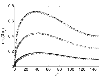
(b)

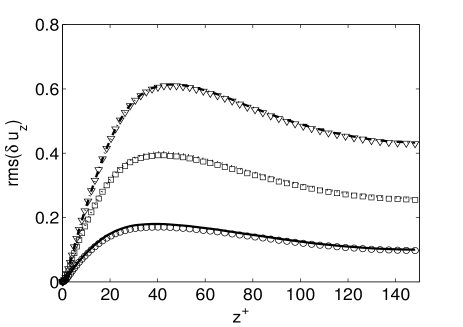
(c)

Figure 7: Rms of the filtering error $\delta{\bf u}$ in the streamwise (a), spanwise (b) and normal (c) directions as a function of $z^{+}$ at varying filter type and width. Profiles refer to the $St=5$ particles.

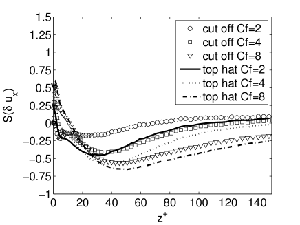
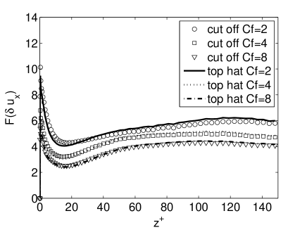
(a)                                                                       (b)

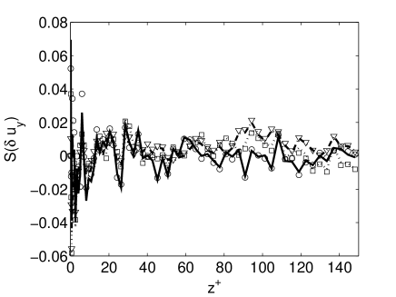
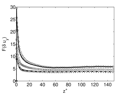
(c)                                                                       (d)

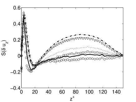
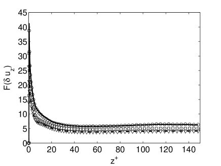
(e)                                                                       (f)

Figure 8: Skewness and flatness of the filtering error $\delta{\bf u}$ in the streamwise (a-b), spanwise (c-d) and wall-normal (e-f) directions as a function of $z^{+}$ at varying filter type and width. Profiles refer to the $St=5$ particles.

Analysis of the higher-order moments also shows that effects due to the filter width are much stronger than those associated with the filter type. No effect of the filter type is observed on the rms of the filtering error, reported in Fig. 7. Profiles change only with the filter width, reaching higher values as CF increases because of the larger amount of fluid velocity fluctuations damped in more coarse-grained fields. Filter type effects are minor also on the skewness and flatness factors, shown in Fig. 8. When the filter width is increased, the skewness factor in the streamwise direction (Fig. 8a) increases to high positive values very close to the wall and decreases to low negative values outside the buffer layer ($z^{+}>30$). In this outer region of the flow, the skewness in the wall-normal direction (Fig. 8e) increases significantly, switching from negative to positive values as CF increases. High positive value of the skewness mean that $\delta{\bf u}$ more frequently attains large positive rather than negative values, and of course the reverse for negative skewness. The largest filter width effects on the flatness factor are observed in the streamwise direction (Fig. 8b) and produce a decrease of $F(\delta u_{x})$ throughout the entire channel: for small and intermediate widths ($CF=2$ and 4) the flatness factor is everywhere higher than 3, for large widths (e.g. $CF=8$) values fall below 3 in the region $10<z^{+}<30$. We remind that high values of the flatness factor, like those characterizing the spanwise direction (Fig. 8d), and the wall-normal direction (Fig. 8f), indicate that error fluctuations are often larger than the variance of the distribution and that error fluctuations have an intermittent character.

IV Probability distribution of the filtering error

In the previous section, we have characterized statistically a lower bound for the error produced by the filtering procedure inherent to the LES approach. This error is intrinsic of LPT in LES flow fields and its mean and higher order moments depend both on particle inertia and on filter width. In this section, we focus on the characterization of the one-point Eulerian probability density function (PDF) of the filtering error. This function can be derived from the more general Lagrangian PDF and is the most practical for direct evaluation of the errors made in the calculation of the statistical momentsPope_2 ; Min_01 . In the frame of the present study, the issues of interest about the PDF of the filtering error can be summarized by the following questions:

1. Is the filtering error deterministic or stochastic?

2. Does it have a simple distribution, for instance Gaussian stochastic?

3. Is it universal or flow-dependent ?

To answer these questions, we consider the PDFs of the streamwise and wall-normal component of the lower-bound filtering error $\delta{\bf u}$. These quantities, indicated hereinafter as $p(\delta u_{x})$ and $p(\delta u_{z})$ respectively, have been computed averaging over the same fluid slabs defined in Sec. III and over the same time interval given in Sec. II.3. In addition, PDFs have been normalized and shifted to be centered around zero: without shifting the profiles, both $p(\delta u_{x})$ and $p(\delta u_{z})$ would be centered around different values of $\delta u_{x}$ and $\delta u_{z}$ for the different particle sets, as a result of the dependence of the filtering error on particle inertia (see Sec. III.1). Probability distributions in the spanwise direction are not shown as they are very similar to those obtained for $p(\delta u_{z})$ and add very little to the discussion.

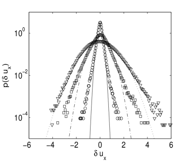
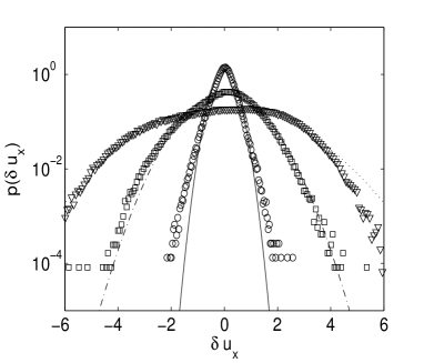
$z^{+}=4.07$	$z^{+}=16.86$
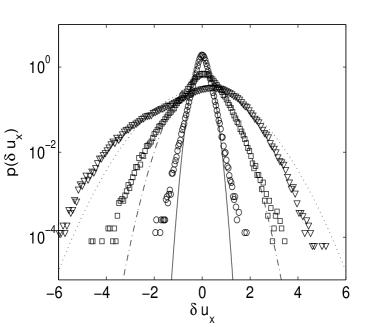
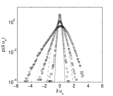
$z^{+}=37.64$	$z^{+}=65.14$

Figure 9: Probability density functions of the streamwise component of the filtering error for different filter widths. Profiles refer to results obtained for the $St=5$ particles with cut-off filter. Open symbols are used for the computed PDFs ($\circ$: CF=2, $\square$: CF=4, $\triangledown$: CF=8); lines for the corresponding Gaussian PDFs ($---$: CF=2, $-\cdot-\cdot-$: CF=4, $\cdot\cdot\cdot\cdot$: CF=8).

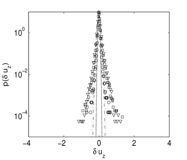
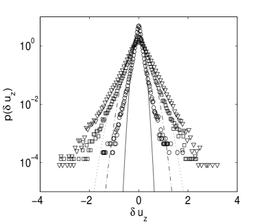
$z^{+}=4.07$	$z^{+}=16.86$
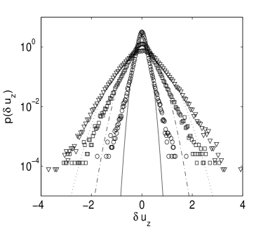
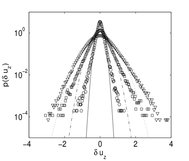
$z^{+}=37.64$	$z^{+}=65.14$

Figure 10: Probability density functions of the wall-normal component of the filtering error for different filter widths. Profiles refer to results obtained for the $St=5$ particles with cut-off filter. Open symbols are used for the computed PDFs ($\circ$: CF=2, $\square$: CF=4, $\triangledown$: CF=8); lines for the corresponding Gaussian PDFs ($---$: CF=2, $-\cdot-\cdot-$: CF=4, $\cdot\cdot\cdot\cdot$: CF=8).

We examine first the PDF behavior at varying filter widths, shown in Figs. 9 and 10. To this aim, we focus on results obtained for the $St=5$ particles when the cut-off filter is used (as for the statistical moments of $\delta{\bf u}$, effects on the PDF behavior due to the filter type appear negligible and hence will not be discussed). In these figures profiles relative to four different distances from the wall are considered to emphasize flow anisotropy effects: clearly, choosing a non-homogeneous anisotropic flow as reference configuration is of particular importance to devise general conclusions. For comparison purposes, the normalized Gaussian distributions (lines) with variance equal to that of the computed PDFs (symbols) at the same wall distance are also shown. A first (expected) result is that the PDF variance increases with the filter width in all flow directions and at all wall-normal locations examined. Another important finding is that, in all cases examined, the error is not deterministic, displays very complex features and covers a wide range of values (typical of probabilistic process) in all cases. Specifically, the PDFs are not Gaussian and their behavior varies strongly with the distance from the wall. This observation is not obvious since the error behavior might be quite different and even perfectly Gaussian in spite of the non-homogeneous nature of the flow. Figs. 9 and 10 show that both $p(\delta u_{x})$ and $p(\delta u_{z})$ are characterized by larger flatness than the corresponding Gaussian distributions for all filter widths and at almost all wall-normal locations. Furthermore, both PDFs are skewed near the wall $-$at $z^{+}\simeq 4$, Figs. 9a and 10a $-$and outside the buffer region $-$at $z^{+}\simeq 65$, Figs. 9d and 10d. This is again related to poor description of coherent structures, e.g. low-speed streaks and turbulent vortices. At intermediate wall-normal locations, PDFs exhibit a nearly Gaussian behavior only at $z^{+}\simeq 17$ for all filter widths but the largest $-$Figs. 9b and 10b; at $z^{+}\simeq 37$, where Reynolds stresses reach a maximum, the non-Gaussian behavior of the PDF profiles increases again $-$Figs. 9c and 10c. It can also be observed that (i) $p(\delta u_{z})$ profiles become flatter at increasing filter widths (Fig. 10), and (ii) filter width effects lead to higher skewness and mildly decreasing flatness of the PDF, consistently with results of Figs. 8a and 8b. For the largest filter width (CF=8), there is a change from positive skewness in the very near wall region ($z^{+}\simeq 4$) to negative skewness away from the wall.

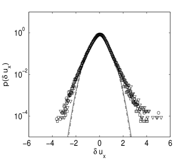
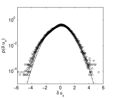
$z^{+}=4.07$	$z^{+}=16.86$
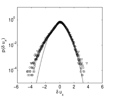
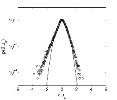
$z^{+}=37.64$	$z^{+}=65.14$

Figure 11: Probability density functions of the streamwise component of the filtering error for different particle inertia. Profiles refer to results obtained using cut-off filter with CF=4. Open symbols are used for the computed PDFs ($\circ$: $St=1$, $\square$: $St=5$, $\triangledown$: $St=25$); lines for the corresponding Gaussian PDFs ($---$: $St=1$, $-\cdot-\cdot-$: $St=5$, $\cdot\cdot\cdot\cdot$: $St=25$).

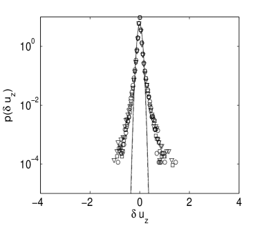
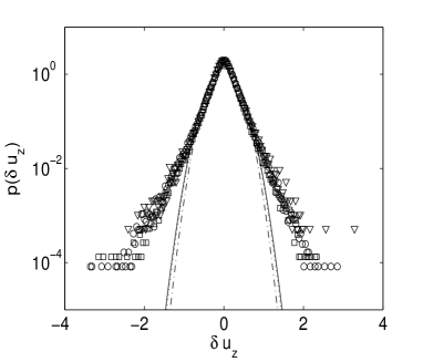
$z^{+}=4.07$	$z^{+}=16.86$
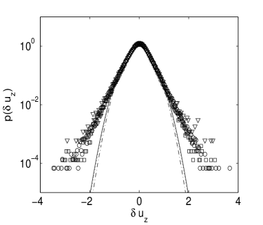
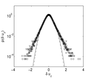
$z^{+}=37.64$	$z^{+}=65.14$

Figure 12: Probability density functions of the wall-normal component of the filtering error for different particle inertia. Profiles refer to results obtained using cut-off filter with CF=4. Open symbols are used for the computed PDFs ($\circ$: $St=1$, $\square$: $St=5$, $\triangledown$: $St=25$); lines for the corresponding Gaussian PDFs ($---$: $St=1$, $-\cdot-\cdot-$: $St=5$, $\cdot\cdot\cdot\cdot$: $St=25$).

Additional information on $p(\delta u_{x})$ and $p(\delta u_{z})$ can be obtained examining how these quantities are modified by particle inertia. To this aim, we focus on results obtained using a cut-off filter with CF=4, shown in Figs. 11 and 12. A first observation is that the effect of inertia on the shape of the PDFs is almost negligible, as we have tried to emphasize by centering all profiles around $\delta u_{i}=0$, where $i=x,z$. A general feature of the PDFs reported in Figs. 11 and 12 is that they exhibit higher tails compared to the corresponding Gaussian distributions, even near the channel center. This is in line with the analysis of the flatness profiles carried out in Sec. III.1. The flatness is larger for the wall-normal probability distributions and varies mildly with the distance from the wall, the only exception being the viscous sublayer (see profiles at $z^{+}\simeq 4$). In terms of relative importance of the PDF tails, $p(\delta u_{x})$ profiles exhibit asymmetries towards negative values of $\delta u_{x}$ which become particularly evident outside the viscous sublayer ($z^{+}\simeq 17$, 37 and 65); whereas $p(\delta u_{z})$ profiles are all symmetric with just a slight asymmetry observed at $z^{+}\simeq 17$. These findings are in agreement with the skewness profiles shown in Figure 5.

Some general conclusions can be drawn from collective analysis of Figs. 9 to 12. First, intrinsic filtering errors of LES in LPT can be described as a stochastic process almost everywhere non-Gaussian with important and long tails (namely large flatness) and appreciable skewness. This process is significantly influenced by flow anisotropy as demonstrated by the dependency of skewness of $p(\delta u_{x})$ on the distance from the wall. This result is important from the modeling viewpoint, as it implies that neither deterministic models nor stochastic homogeneous models have the capability to correct fully intrinsic error made in the LES approach due to filtering. Second, the model should adapt dynamically over space to account for local inhomogeneity and anisotropy of the flow and to reproduce the correct crossing trajectory effect: this latter effect, in particular, is due to the existence of a mean relative particle-to-fluid velocity (rather than an instantaneous one) associated with the lack of correlation between the fluid velocity seen by the inertial particles and the velocity of fluid particles Min_04 . Finally, results demonstrate that a mandatory requirement to scrutinize model performance is the capability to reproduce correctly all spatial turbulent structures (or at least their statistical effect).

V Concluding Remarks

In this work, we proposed a simple procedure to characterize the filtering error intrinsic of Lagrangian particle tracking in LES flow fields. Specifically, we focused on the error purely due to filtering of the fluid velocity fields seen by the particles, for which we quantified a lower bound. This “minimum” error can not be avoided but potentially can be corrected. To this aim, we considered an ideal situation in which the exact dynamics of the resolved velocity field is available and time accumulation of the pure filtering error on particle trajectories is eliminated a-priori. Evaluation of the statistical properties of the filtering error has been performed applying filters of different type and different widths, corresponding roughly to varying amounts of resolved flow energy, and considering heavy particles with different inertia. In particular, mean and higher-order moments as well as one-point probability distribution functions have been analyzed to provide information about the key features required in SGS models for Lagrangian particle tracking to compensate for such error.

The first interesting result is that the mean value of the filtering error components along particle trajectories is not zero, as it would be obtained performing an Eulerian analysis of filtering effects at fixed points. Non-zero mean values result from filtering effects on the coherent turbulent structures which characterize the near-wall region and are preferentially sampled by the inertial particles. Smoothing of the low-speed streaks due to filtering is associated with a near-wall negative peak of the mean filtering error in the streamwise direction. Filtering effects on the near-wall vortical structures, and in turn on sweep and ejection events, lead to even more complicated mean profiles in the wall-normal direction: in this case, a near-wall positive peak followed by a negative peak farther from the wall is observed. In both directions, particle inertia and filter width change significantly the qualitative behavior of the error. Mean value analysis confirms that the error introduced by filtering on inertial particle motion is not just yield by the reduction of fluid velocity fluctuations, a well-known effect pointed out in Eulerian error analyses in LES. This supports the conclusion, drawn in our previous worksMarchioli2008 ; Marchioli2008b , that SGS model for the particle equations can not ensure accurate prediction of particle preferential concentration and near-wall accumulation by only reintroducing the correct amount of fluid velocity fluctuations. Improved predictions of LES applied to turbulent dispersed flow necessitate suitable benchmarks against statistical information at the sub-grid level, and the present study establishes precisely the minimum benchmarking requirements.

Joint analysis of the the higher-order statistical moments and of the probability distribution functions shows that the filtering error distribution differs significantly from a normalized Gaussian distribution with the same variance. All error components are characterized by a flatness generally larger than the Gaussian value of 3. The streamwise and wall-normal components are also characterized by skewed distributions, not observed in the spanwise direction: both positive and negative skewness values can be attained depending on the distance from the wall. This indicates that error behavior is intermittent and strongly affected by flow anisotropy. Changes in the probability distributions are also found at varying filter width. Besides the expected increase of the variance of the PDF when the filter become coarser, noticeable effects are observed on the skewness and flatness of the streamwise PDF and on the skewness of the wall-normal PDF. No significant effects are observed when either filter type or particle inertia are changed.

Present results emphasize the stochastic nature of the pure filtering error. In our opinion, a possible way to correct this error could be represented by a generalized stochastic Lagrangian model pope ; Min_01 in which the statistical signature of coherent turbulent structures (e.g. low-speed streaks, sweeps and ejections) on particle dynamics is accounted for explicitly. In this perspective, the filtering error characterization and quantification provided by the present study represents a valuable tool to understand how these structures are affected by filtering and how sub-grid scale fluid velocities impact the force driving the particles. Models of this type have already been developed in the context of RANS methods Min_04 , followed by extensions to heuristic particle deposition modelingChi_08 and by first attempts at explicitly modeling the statistical effects of structures on particle statistics in near-wall regionsGui_08 . Much work remains to be done. The first necessary step is of course to extend the formalism to the LES framework. To this aim, a detailed Lagrangian analysis of the error should be performed to complement present results and assist in model development.

List of Tables

Table 1: Particle parameters; $\tau_{p}$ is the particle relaxation time, $d_{p}$ the particle diameter, $V_{s}$ the particle settling velocity and $Re_{p}$ the particle Reynolds number. The superscript $+$ denotes the corresponding quantities expressed in wall units.

$St$	$\tau_{p}~{}(s)$	$d_{p}^{+}$	$d_{p}$ (${\mu}m$)	$V_{s}^{+}=g^{+}\cdot St$	$Re_{p}^{+}=V_{s}^{+}\cdot d_{p}^{+}/\nu^{+}$
1	$1.133\cdot 10^{-3}$	$0.153$	$~{}20.4$	$0.0943$	$0.01443$
5	$5.660\cdot 10^{-3}$	$0.342$	$~{}45.6$	$0.4717$	$0.16132$
25	$28.32\cdot 10^{-3}$	$0.765$	$102.0$	$2.3584$	$1.80418$

Table 1: Particle parameters; $\tau_{p}$ is the particle relaxation time, $d_{p}$ the particle diameter, $V_{s}$ the particle settling velocity and $Re_{p}$ the particle Reynolds number. The superscript $+$ denotes the corresponding quantities expressed in wall units.

List of Figures

Figure 1: Mean values of the filtering error $\delta{\bf u}$ in the streamwise (a), spanwise (b) and wall-normal (c) directions as a function of $z^{+}$ at varying particle inertia. Profiles refer to the cut-off filter with CF=4.
Figure 2: Fluid streaks in the near-wall region. Low-speed (resp. high-speed) streaks are rendered using colored contours of negative (resp. positive) streamwise fluctuating velocity $u_{x}^{\prime}$ on a horizontal plane at $z^{+}=10$ from the wall. Panel (a) shows the streaky structures obtained from DNS; the instantaneous distribution of the $St=25$ particles comprised between $z^{+}=10$ and the wall is also shown to highlight preferential distribution into the low-speed streaks. Panels (b) and (c) show the streaky structures obtained from a-priori DNS with coarsening-factor 4 and 8, respectively.
Figure 3: Effects of filtering on the mean wall-normal fluid velocity seen by the particles at varying particle inertia. Profiles refer to the cut-off filter with CF=4.
Figure 4: Rms of the filtering error $\delta{\bf u}$ in the streamwise (a), spanwise (b) and wall-normal (c) directions as a function of $z^{+}$ at varying particle inertia. Profiles refer to the cut-off filter with CF=4.
Figure 5: Skewness and flatness of the filtering error $\delta{\bf u}$ in the streamwise (a-b), spanwise (c-d) and wall-normal (e-f) directions as a function of $z^{+}$ at varying particle inertia. Profiles refer to the cut-off filter with CF=4.
Figure 6: Mean values of the filtering error $\delta{\bf u}$ in the streamwise (a), and wall-normal (b) directions as a function of $z^{+}$ at varying filter type and width. Profiles refer to the $St=5$ particles.
Figure 7: Rms of the filtering error $\delta{\bf u}$ in the streamwise (a), spanwise (b) and normal (c) directions as a function of $z^{+}$ at varying filter type and width. Profiles refer to the $St=5$ particles.
Figure 8: Skewness and flatness of the filtering error $\delta{\bf u}$ in the streamwise (a-b), spanwise (c-d) and wall-normal (e-f) directions as a function of $z^{+}$ at varying filter type and width. Profiles refer to the $St=5$ particles.
Figure 9: Probability density functions of the streamwise component of the filtering error for different filter widths. Profiles refer to results obtained for the $St=5$ particles with cut-off filter. Open symbols are used for the computed PDFs ($\circ$: CF=2, $\square$: CF=4, $\triangledown$: CF=8); lines for the corresponding Gaussian PDFs ($---$: CF=2, $-\cdot-\cdot-$: CF=4, $\cdot\cdot\cdot\cdot$: CF=8).
Figure 10: Probability density functions of the wall-normal component of the filtering error for different filter widths. Profiles refer to results obtained for the $St=5$ particles with cut-off filter. Open symbols are used for the computed PDFs ($\circ$: CF=2, $\square$: CF=4, $\triangledown$: CF=8); lines for the corresponding Gaussian PDFs ($---$: CF=2, $-\cdot-\cdot-$: CF=4, $\cdot\cdot\cdot\cdot$: CF=8).
Figure 11: Probability density functions of the streamwise component of the filtering error for different particle inertia. Profiles refer to results obtained using cut-off filter with CF=4. Open symbols are used for the computed PDFs ($\circ$: $St=1$, $\square$: $St=5$, $\triangledown$: $St=25$); lines for the corresponding Gaussian PDFs ($---$: $St=1$, $-\cdot-\cdot-$: $St=5$, $\cdot\cdot\cdot\cdot$: $St=25$).
Figure 12: Probability density functions of the wall-normal component of the filtering error for different particle inertia. Profiles refer to results obtained using cut-off filter with CF=4. Open symbols are used for the computed PDFs ($\circ$: $St=1$, $\square$: $St=5$, $\triangledown$: $St=25$); lines for the corresponding Gaussian PDFs ($---$: $St=1$, $-\cdot-\cdot-$: $St=5$, $\cdot\cdot\cdot\cdot$: $St=25$).

References

- [1] L. P. Wang and M. R. Maxey, “Settling velocity and concentration distribution of heavy particles in homogeneous isotropic turbulence,” J. Fluid Mech. 256, 27 (1993).
- [2] C. Marchioli and A. Soldati, “Mechanisms for particle transfer and segregation in turbulent boundary layer,” J. Fluid Mech. 468, 283 (2002).
- [3] J. Bec, L. Biferale, M. Cencini, A. Lanotte, S. Musacchio and F. Toschi, “Heavy particle concentration in turbulence at dissipative and inertial scales,” Phys. Rev. Lett. 98, 084502 (2007).
- [4] P. Fede and O. Simonin, “Numerical study of the subgrid fluid turbulence effects on the statistics of heavy colliding particles,” Phys. Fluids 18, 045103 (2006).
- [5] D. W. Rouson and J. K. Eaton, “On the preferential concentration of solid particles in turbulent channel flow,” J. Fluid Mech. 428, 149 (2001).
- [6] A. Soldati and C. Marchioli, “Physics and modelling of turbulent particle deposition and entrainment: review of a systematic study,” Int. J. Multiphase Flow 20, 827 (2009).
- [7] C. Marchioli, A. Giusti, M. V. Salvetti and A. Soldati, “Direct numerical simulation of particle wall transfer and deposition in upward turbulent pipe flow,” Int. J. Multiphase Flow 29, 1017 (2003).
- [8] W. S. J. Uijttewaal and R. W. A. Oliemans, “Particle dispersion and deposition in direct numerical and large eddy simulations of vertical pipe flows,” Phys. Fluids 8, 2590 (1996).
- [9] S.V. Apte, K. Mahesh, P. Moin and J. Oefelein, “Large-eddy simulation of swirling particle-laden flows in a coaxial-jet combustor,” Int. J. Multiphase Flow 29, 1311 (2003).
- [10] N.A. Okongo and J. Bellan, “Consistent large-eddy simulation of a temporal mixing layer laden with evaporating drops. Part 1. direct numerical simulation, formulation and a priori analysis,” J. Fluid Mech. 499, 1 (2004).
- [11] J. G. M. Kuerten and A. W. Vreman, “Can turbophoresis be predicted by large-eddy simulation?,” Phys. Fluids 17, 011701 (2005).
- [12] J. G. M. Kuerten, “Subgrid modeling in particle-laden channel flow,” Phys. Fluids 18, 025108 (2006).
- [13] C. Marchioli, M. V. Salvetti and A. Soldati, “Some issues concerning large-eddy simulation of inertial particle dispersion in turbulent bounded flows,” Phys. Fluids 20, 040603 (2008).
- [14] M. A. I. Khan, X. Y. Luo, F. C. G. A. Nicolleau, P. G. Tucker and G. Lo Iacono, “Effects of LES sub-grid flow structure on particle deposition in a plane channel with a ribbed wall,” International Journal for Numerical Methods in Biomedical Engineering 26, 999 (2010).
- [15] B. Shotorban and F. Mashayek, “Modeling subgrid-scale effetcs on particles by approximate deconvolution,” Phys. Fluids 17, 081701 (2005).
- [16] C. Gobert, “Analytical assessment of models for large eddy simulation of particle laden flow,” J. Turbulence 11, 1 (2010).
- [17] C. Marchioli, M.V. Salvetti and A. Soldati, “Appraisal of energy recovering sub-grid scale models for large-eddy simulation of turbulent dispersed flows,” Acta Mech. 201(1-4), 277 (2008).
- [18] B. Shotorban and F. Mashayek,, “A stochastic model for particle motion in large-eddy simulation.,” J. Turbulence 7, N18 (2006).
- [19] J. Pozorski and S.V. Apte, “Filtered particle tracking in isotropic turbulence and stochastic modeling of subgrid-scale dispersion,” Int. J. Multiphase Flow 35, 118 (2008).
- [20] E. Calazavarini, A. Donini, V. Lavezzo, C. Marchioli, E. Pitton, A. Soldati and F. Toschi, “On the error estimate in the sub-grid models for particles in turbulent flows,” Direct and Large-Eddy Simulation 8, Eindhoven - The Netherlands July 7-9, 2010.
- [21] S. E. Elghobashi and G. C. Truesdell, “Direct simulation of particle dispersion in a decaying isotropic turbulence,” J. Fluid Mech. 242, 655 (1992).
- [22] R. Gatignol, ”The Fax n formulae for a rigid particle in an unsteady non-uniform Stokes flow,” J. Mec. Theor. Appl. 1, 143 (1983).
- [23] Y. Pan and S. Banerjee, “Numerical simulation of particle interactions with wall turbulence,” Phys. Fluids 17, 2733 (1996).
- [24] S. Pope, “Ten questions concerning the large-eddy simulation of turbulent flows,” New J. Phys. 6, 1 (2004).
- [25] M. Picciotto, C. Marchioli, M.W. Reeks and A. Soldati, “Statistics of velocity and preferential accumulation of micro-particles in boundary layer turbulence,” Nuclear Eng. Design 235, 1239 (2005).
- [26] M. Picciotto, C. Marchioli and A. Soldati, “Characterization of near-wall accumulation regions for inertial particles in turbulent boundary layers,” Phys. Fluids 17, 098101(2005).
- [27] C. Marchioli, M.V. Salvetti and A. Soldati, ”Inertial particle segregation and deposition in large-eddy simulation of turbulent wall-bounded flows,”’ Quality and Reliability of Large-Eddy Simulations II, Ercoftac Series, Eds. M.V. Salvetti, B.J. Geurts, J. Meyers and P. Sagaut, Springer (2011).
- [28] S.B. Pope. Turbulent Flows. Cambridge University Press, Cambridge (2000).
- [29] J-P. Minier and E. Peirano, ”The PDF approach to polydispersed turbulent two-phase flows” Physics Reports 352, 1, (2001).
- [30] J.P. Minier, E. Peirano and S. Chibbaro, “PDF model based on Langevin equation for polydispersed two-phase flows applied to a bluff-body gas-solid flow”, Phys. Fluids 16, 2419 (2004).
- [31] Pope, S. “Simple models for turbulent flows,” Phys. Fluids, 23, 011301 (2011).
- [32] S Chibbaro, and J.P. Minier, “Langevin PDF simulation of particle deposition in a turbulent pipe flow”, Journal of Aerosol Science 39, 555 (2008).
- [33] M. Guingo and J-P. Minier “A stochastic model of coherent structures for particle deposition in turbulent flows”, Phys. Fluids 20, 053303(2008).