An Oracle-based, Output-sensitive Algorithm
for Projections of Resultant Polytopes

Abstract

We design an algorithm to compute the Newton polytope of the resultant, known as resultant polytope, or its orthogonal projection along a given direction. The resultant is fundamental in algebraic elimination, optimization, and geometric modeling. Our algorithm exactly computes vertex- and halfspace-representations of the polytope using an oracle producing resultant vertices in a given direction, thus avoiding walking on the polytope whose dimension is $\alpha-n-1$, where the input consists of $\alpha$ points in ${\mathbb{Z}}^{n}$. Our approach is output-sensitive as it makes one oracle call per vertex and facet. It extends to any polytope whose oracle-based definition is advantageous, such as the secondary and discriminant polytopes. Our publicly available implementation uses the experimental CGAL package triangulation. Our method computes $5$-, $6$- and $7$-dimensional polytopes with $35$K, $23$K and $500$ vertices, respectively, within $2$hrs, and the Newton polytopes of many important surface equations encountered in geometric modeling in $<1$sec, whereas the corresponding secondary polytopes are intractable. It is faster than tropical geometry software up to dimension $5$ or $6$. Hashing determinantal predicates accelerates execution up to $100$ times. One variant computes inner and outer approximations with, respectively, 90% and 105% of the true volume, up to $25$ times faster.

Keywords:

General Dimension, Convex Hull, Regular Triangulation, Secondary Polytope, Resultant, CGAL Implementation, Experimental Complexity.

1 Introduction

Given pointsets $A_{0},\dots,A_{n}\subset{\mathbb{Z}}^{n}$, we define the pointset

$${\mathcal{A}}:=\bigcup_{i=0}^{n}(A_{i}\times\{e_{i}\})\subset{\mathbb{Z}}^{2n},$$ (1)

where $e_{0},\ldots,e_{n}$ form an affine basis of ${\mathbb{R}}^{n}$: $e_{0}$ is the zero vector,$e_{i}=(0,\dots,0,1,0,\dots,0),i=1,\dots,n$. Clearly, $|{\mathcal{A}}|=|A_{0}|+\cdots+|A_{n}|$, where $|\cdot|$ denotes cardinality. By Cayley’s trick (Proposition 2) the regular tight mixed subdivisions of the Minkowski sum $A_{0}+\cdots+A_{n}$ are in bijection with the regular triangulations of ${\mathcal{A}}$, which are in bijection with the vertices of the secondary polytope $\Sigma({\mathcal{A}})$ (see Section 2).

The Newton polytope of a polynomial is the convex hull of its support, i.e. the exponent vectors of monomials with nonzero coefficient. It subsumes the notion of degree for sparse multivariate polynomials by providing more precise information (see Figures 1 and 3). Given $n+1$ polynomials in $n$ variables, with fixed supports $A_{i}$ and symbolic coefficients, their sparse (or toric) resultant ${\mathcal{R}}$ is a polynomial in these coefficients which vanishes exactly when the polynomials have a common root (Definition 1). The resultant is the most fundamental tool in elimination theory, it is instrumental in system solving and optimization, and is crucial in geometric modeling, most notably for changing the representation of parametric hypersurfaces to implicit.

The Newton polytope of the resultant $N({\mathcal{R}})$, or resultant polytope, is the object of our study; it is of dimension $|{\mathcal{A}}|-2n-1$ (Proposition 4). We further consider the case when some of the input coefficients are not symbolic, hence we seek an orthogonal projection of the resultant polytope. The lattice points in $N({\mathcal{R}})$ yield a superset of the support of ${\mathcal{R}}$; this reduces implicitization ^{1, 2} and computation of ${\mathcal{R}}$ to sparse interpolation (Section 2). The number of coefficients of the $n+1$ polynomials ranges from $O(n)$ for sparse systems, to $O(n^{d}d^{n})$, where $d$ bounds their total degree. In system solving and implicitization, one computes ${\mathcal{R}}$ when all but $O(n)$ of the coefficients are specialized to constants, hence the need for resultant polytope projections.

The resultant polytope is a Minkowski summand of $\Sigma({\mathcal{A}})$, which is also of dimension $|{\mathcal{A}}|-2n-1$. We consider an equivalence relation defined on the $\Sigma({\mathcal{A}})$ vertices, where the classes are in bijection with the vertices of the resultant polytope. This yields an oracle producing a resultant vertex in a given direction, thus avoiding to compute $\Sigma({\mathcal{A}})$, which typically has much more vertices than $N({\mathcal{R}})$. This is known in the literature as an optimization oracle since it optimizes inner product with a given vector over the (unknown) polytope.

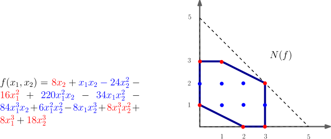
Figure 1: The Newton polytope of a polynomial of degree $5$ in two variables. Every monomial corresponds to an integral point on the plane. The dashed triangle is the corresponding polytope of the dense polynomial of degree $5$.

Example 1.

[The bicubic surface] A standard benchmark in geometric modeling is the implicitization of the bicubic surface, with $n=2$, defined by $3$ polynomials in two parameters. The input polynomials have supports $A_{i}\subset{\mathbb{Z}}^{2},\,i=0,1,2$, with cardinalities $7,6,14$, respectively; the total degrees are $3,3,6$, respectively. The Cayley set ${\mathcal{A}}\subset{\mathbb{Z}}^{4}$, constructed as in Equation 1, has $7+6+14=27$ points. It is depicted in the following matrix, with coordinates as columns, where the supports from different polynomials and the Cayley coordinates are distinguished. By Proposition 4 it follows that $N({\mathcal{R}})$ has dimension $|{\mathcal{A}}|-4-1=22$; it lies in ${\mathbb{R}}^{27}$.

$0$ $0$ $1$ $0$ $2$ $0$ $3$ $0$ $0$ $1$ $2$ $0$ $3$ $0$ $0$ $1$ $0$ $1$ $2$ $1$ $2$ $1$ $2$ $3$ $2$ $3$ $3$ } support

$0$ $1$ $0$ $2$ $0$ $3$ $0$ $0$ $1$ $0$ $0$ $3$ $0$ $0$ $1$ $0$ $2$ $1$ $0$ $2$ $1$ $3$ $2$ $1$ $3$ $2$ $3$

$0$ $0$ $0$ $0$ $0$ $0$ $0$ $1$ $1$ $1$ $1$ $1$ $1$ $0$ $0$ $0$ $0$ $0$ $0$ $0$ $0$ $0$ $0$ $0$ $0$ $0$ $0$ } Cayley

$0$ $0$ $0$ $0$ $0$ $0$ $0$ $0$ $0$ $0$ $0$ $0$ $0$ $1$ $1$ $1$ $1$ $1$ $1$ $1$ $1$ $1$ $1$ $1$ $1$ $1$ $1$

Implicitization requires eliminating the two parameters to obtain a constraint equation over the symbolic coefficients of the polynomials. Most of the coefficients are specialized except for $3$ variables, hence the sought for implicit equation of the surface is trivariate and the projection of $N({\mathcal{R}})$ lies in ${\mathbb{R}}^{3}$.

TOPCOM ³ needs more than a day and $9$GB of RAM to compute $1,806,467$ regular triangulations of ${\mathcal{A}}$, corresponding to $29$ of the vertices of $N({\mathcal{R}})$, and crashes before computing the entire $N({\mathcal{R}})$. Our algorithm yields the projected vertices $\{(0,0,1),(0,1,0),$ $(1,0,0),(0,0,9),(0,18,0),(18,0,0)\}$ of the $3$-dimensional projection of $N({\mathcal{R}})$, which is the Newton polytope of the implicit equation, in $30$msec. Given this polytope, the implicit equation of the bicubic surface is interpolated in 42 seconds ⁴. It is a polynomial of degree $18$ containing $715$ terms which corresponds exactly to the lattice points contained in the predicted polytope.

Our main contribution is twofold. First, we design an oracle-based algorithm for computing the Newton polytope of $\mathcal{R}$, or of specializations of ${\mathcal{R}}$. The algorithm utilizes the Beneath-and-Beyond method to compute both vertex (V) and halfspace (H) representations, which are required by the algorithm and may also be relevant for the targeted applications. Its incremental nature implies that we also obtain a triangulation of the polytope, which may be useful for enumerating its lattice points. The complexity is proportional to the number of output vertices and facets; in this sense, the algorithms is output sensitive. The overall cost is asymptotically dominated by computing as many regular triangulations of ${\mathcal{A}}$ (Theorem 1). We work in the space of the projected $N({\mathcal{R}})$ and revert to the high-dimensional space of $\Sigma({\mathcal{A}})$ only if needed. Our algorithm readily extends to computing $\Sigma({\mathcal{A}})$, the Newton polytope of the discriminant and, more generally, any polytope that can be efficiently described by a vertex oracle or its orthogonal projection. In particular, it suffices to replace our oracle by the oracle in Ref. 5 to obtain a method for computing the discriminant polytope.

Second, we describe an efficient, publicly available implementation based on CGAL ⁶ and its experimental package triangulation. Our method computes instances of $5$-, $6$- or $7$-dimensional polytopes with $35$K, $23$K or $500$ vertices, respectively, in $<2$hr. Our code is faster up to dimensions $5$ or $6$, compared to a method computing $N({\mathcal{R}})$ via tropical geometry, implemented in the Gfan library ⁷. In higher dimensions Gfan seems to perform better although neither implementation can compute enough instances for a fair comparison. Our code, in the critical step of computing the convex hull of the resultant polytope, uses triangulation. On our instances, triangulation, compared to state-of-the-art software lrs, cdd, and polymake, is the fastest together with polymake. We factor out repeated computation by reducing the bulk of our work to a sequence of determinants: this is often the case in high-dimensional geometric computing. Here, we exploit the nature of our problem and matrix structure to capture the similarities of the predicates, and hash the computed minors which are needed later, to speedup subsequent determinants. A variant of our algorithm computes successively tighter inner and outer approximations: when these polytopes have, respectively, 90% and 105% of the true volume, runtime is reduced up to $25$ times. This may lead to an approximation algorithm.

Previous work.

Sparse (or toric) elimination theory was introduced in Ref. 8. They show that $N({\mathcal{R}})$, for two univariate polynomials with $k_{0}+1,k_{1}+1$ monomials, has $\binom{k_{0}+k_{1}}{k_{0}}$ vertices and, when both $k_{i}\geq 2$, it has $k_{0}k_{1}+3$ facets. In Section 6 of Ref. 9 is proven that $N({\mathcal{R}})$ is $1$-dimensional if and only if $|A_{i}|=2$, for all $i$, the only planar $N({\mathcal{R}})$ is the triangle, whereas the only $3$-dimensional ones are the tetrahedron, the square-based pyramid, and the resultant polytope of two univariate trinomials; we compute an affinely isomorphic instance of the latter (Figure 2(b)) as the resultant polytope of three bivariate polynomials. Following Theorem 6.2 of Ref. 9, the $4$-dimensional polytopes include the 4-simplex, some $N({\mathcal{R}})$ obtained by pairs of univariate polynomials, and those of 3 trinomials, which have been investigated with our code in Ref. 10. The maximal (in terms of number of vertices) such polytope we have computed has f-vector $(22,66,66,22)$ (Figure 2(c)). Furthermore, Table 2 presents some typical f-vectors of $4,5,6$-dimensional projections of resultant polytopes.

A lower bound on the volume of the Newton polytope of the discriminant polynomial that refutes a conjecture in algebraic geometry is presented in Ref. 11.

A direct approach for computing the vertices of $N({\mathcal{R}})$ might consider all vertices of $\Sigma({\mathcal{A}})$ since the vertices of the former are equivalence classes over the vertices of the latter. Its complexity grows with the number of vertices of $\Sigma({\mathcal{A}})$, hence is impractical (Example 1).

The computation of secondary polytopes has been efficiently implemented in TOPCOM ³, which has been the reference software for computing regular or all triangulations. The software builds a search tree with flips as edges over the vertices of $\Sigma(A)$. This approach is limited by space usage. To address this, reverse search was proposed ¹², but the implementation cannot compete with TOPCOM. The approach based on computing $\Sigma({\mathcal{A}})$ is not efficient for computing $N({\mathcal{R}})$. For instance, in implicitizing parametric surfaces with up to $100$ terms, which includes all common instances in geometric modeling, we compute the Newton polytope of the equations in less than $1$sec, whereas $\Sigma({\mathcal{A}})$ is intractable (see e.g. Example 1).

In Ref. 13 they describe all Minkowski summands of $\Sigma(A)$. In Ref. 14 is defined an equivalence class over $\Sigma(A)$ vertices having the same mixed cells. The classes map in a many-to-one fashion to resultant vertices; our algorithm exploits a stronger equivalence relationship.

Tropical geometry is a polyhedral analogue of algebraic geometry and can be viewed as generalizing sparse elimination theory. It gives alternative ways of recovering resultant polytopes ⁷ and Newton polytopes of implicit equations ². See Section 5 for comparisons of the software in Ref. 7, called Gfan, with our software. In Ref. 5, tropical geometry is used to define vertex oracles for the Newton polytope of the discriminant polynomial.

In Ref. 15 there is a general implementation of a Beneath-and-Beyond based procedure which reconstructs a polytope given by a vertex oracle. This implementation, as reported in Ref. 7, is outperformed by Gfan, especially in dimensions higher than $5$.

As is typical in computational geometry, the practical bottleneck is in computing determinantal predicates. For determinants, the record bit complexity is $O(n^{2.697})$ ¹⁶, while more specialized methods exist for the sign of general determinants, e.g. Ref. 17. These results are relevant for higher dimensions and do not exploit the structure of our determinantal predicates, nor the fact that we deal with sequences of determinants whose matrices are not very different (this is formalized and addressed in Section 4). We compared linear algebra libraries LinBox ¹⁸ and Eigen ¹⁹, which seem most suitable in dimension greater than $100$ and medium to high dimensions, respectively, whereas CGAL provides the most efficient determinant computation for the dimensions to which we focus.

The roadmap of the paper follows: Section 2 describes the combinatorics of resultants, and the following section presents our algorithm. Section 4 overcomes the bottleneck of Orientation predicates. Section 5 discusses the implementation, experiments, and comparison with other software. We conclude with future work.

A preliminary version containing most of the presented results appeared in Ref. 20. This extended version contains a more detailed presentation of the background theory of resultants, applications and examples, a more complete account of previous work, omitted proofs, an improved description of the approximation algorithm, an extended version of the hashing determinants method, and more experimental results.

2 Resultant polytopes and their projections

We introduce tools from combinatorial geometry ^{21, 22} to describe resultants ^{8, 23}. We shall denote by vol$(\cdot)\in{\mathbb{R}}$ the normalized Euclidean volume, $({\mathbb{R}}^{m})^{\times}$ the linear $m$-dimensional functionals, $\mbox{Aff}(\cdot)$ the affine hull, and $\mbox{CH}(\cdot)$ the convex hull.

Let ${\mathcal{A}}\subset{\mathbb{R}}^{d}$ be a pointset whose convex hull is of dimension $d$. For any triangulation $T$ of ${\mathcal{A}}$, define vector $\phi_{T}\in{\mathbb{R}}^{|{\mathcal{A}}|}$ with coordinate

$$\phi_{T}(a)=\sum_{\sigma\in T:a\in\sigma}\mbox{vol}(\sigma),\qquad a\in{\mathcal{A}},$$ (2)

summing over all simplices $\sigma$ of $T$ having $a$ as a vertex; $\Sigma({\mathcal{A}})$ is the convex hull of $\phi_{T}$ for all triangulations $T$. Let ${\mathcal{A}}^{w}$ denote pointset ${\mathcal{A}}$ lifted to ${\mathbb{R}}^{d+1}$ via a generic lifting function $w$ in $({\mathbb{R}}^{|{\mathcal{A}}|})^{\times}$. Regular triangulations of ${\mathcal{A}}$ are obtained by projecting the upper (or lower) hull of ${\mathcal{A}}^{w}$ back to ${\mathbb{R}}^{d}$.

Proposition 1.

[Ref. 8] The vertices of $\Sigma({\mathcal{A}})$ correspond to the regular triangulations of ${\mathcal{A}}$, while its face lattice corresponds to the poset of regular polyhedral subdivisions of ${\mathcal{A}}$, ordered by refinement. A lifting vector produces a regular triangulation $T$ (resp. a regular polyhedral subdivision of ${\mathcal{A}}$) if and only if it lies in the normal cone of vertex $\phi_{T}$ (resp. of the corresponding face) of $\Sigma({\mathcal{A}})$. The dimension of $\Sigma({\mathcal{A}})$ is $|{\mathcal{A}}|-d-1$.

Let $A_{0},\ldots,A_{n}$ be subsets of ${\mathbb{Z}}^{n}$, $P_{0},\ldots,P_{n}\subset{\mathbb{R}}^{n}$ their convex hulls, and $P=P_{0}+\cdots+P_{n}$ their Minkowski sum. A Minkowski (maximal) cell of $P$ is any full-dimensional convex polytope $B=\sum_{i=0}^{n}B_{i}$, where each $B_{i}$ is a convex polytope with vertices in $A_{i}$. Minkowski cells $B,B^{\prime}=\sum_{i=0}^{n}B_{i}^{\prime}$ intersect properly when $B_{i}\cap B_{i}^{\prime}$ is a face of both and their Minkowski sum descriptions are compatible, i.e. coincide on the common face. A mixed subdivision of $P$ is any family of Minkowski cells which partition $P$ and intersect properly. A Minkowski cell is $i$-mixed or $v_{i}$-mixed, if it is the Minkowski sum of $n$ one-dimensional segments from $P_{j},\,j\neq i$, and some vertex $v_{i}\in P_{i}$. In the sequel we shall call a Minkowski cell, simply cell.

Mixed subdivisions contain faces of all dimensions between 0 and $n$, the maximum dimension corresponding to cells. Every face of a mixed subdivision of $P$ has a unique description as Minkowski sum of $B_{i}\subset P_{i}$. A mixed subdivision is regular if it is obtained as the projection of the upper (or lower) hull of the Minkowski sum of lifted polytopes $P_{i}^{w_{i}}:=\{(p_{i},w_{i}(p_{i}))~{}|~{}p_{i}\in P_{i}\}$, for lifting $w_{i}:P_{i}\rightarrow{\mathbb{R}}$. If the lifting function $w:=(w_{0}\ldots,w_{n})$ is sufficiently generic, then the mixed subdivision is tight, and $\sum_{i=0}^{n}\dim B_{i}=\dim\sum_{i=0}^{n}B_{i}$, for every cell. Given $A_{0},\ldots,A_{n}$ and the affine basis $\{e_{0},\ldots,e_{n}\}$ of ${\mathbb{R}}^{n}$, we define the Cayley pointset ${\mathcal{A}}\subset{\mathbb{Z}}^{2n}$ as in equation (1).

Proposition 2.

[Cayley trick, Ref. 8] There exist bijections between: the regular tight mixed subdivisions of $P$ and the regular triangulations of ${\mathcal{A}}$; the tight mixed subdivisions of $P$ and the triangulations of ${\mathcal{A}}$; the mixed subdivisions of $P$ and the polyhedral subdivisions of ${\mathcal{A}}$.

The family $A_{0},\dots,A_{n}\subset{\mathbb{Z}}^{n}$ is essential if they jointly affinely span ${\mathbb{Z}}^{n}$ and every subset of cardinality $j,1\leq j<n$, spans a space of dimension greater than or equal to $j$. It is straightforward to check this property algorithmically and, if it does not hold, to find an essential subset ⁹. In the sequel, the input $A_{0},\dots,A_{n}\subset{\mathbb{Z}}^{n}$ is supposed to be essential. Given a finite $A\subset{\mathbb{Z}}^{n}$, we denote by ${\mathbb{C}}^{A}$ the space of all Laurent polynomials of the form $\sum_{a\in A}c_{a}x^{a},c_{a}\neq 0,x=(x_{1},\ldots,x_{n})$. Similarly, given $A_{0},\dots,A_{n}\subset{\mathbb{Z}}^{n}$ we denote by $\prod_{i=0}^{n}{\mathbb{C}}^{A_{i}}$ the space of all systems of polynomials

$$f_{0}=f_{1}=\dots=f_{n}=0,$$ (3)

where $\sum_{a\in A_{i}}c_{i,a}x^{a},c_{i,a}\neq 0$. The vector of all coefficients $(\ldots,c_{i,a},\ldots)$ of (3) defines a point in $\prod_{i=0}^{n}{\mathbb{C}}^{A_{i}}$. Let $Z\subset\prod_{i=0}^{n}{\mathbb{C}}^{A_{i}}$ be the set of points corresponding to systems (3) which have a solution in $({\mathbb{C}}^{*})^{n}$, and let $\overline{Z}$ be its closure. $\overline{Z}$ is an irreducible variety defined over ${\mathbb{Q}}$.

Definition 1.

If codim$(\overline{Z})=1$, then the sparse (or toric) resultant of the system of polynomials (3) is the unique (up to sign) polynomial ${\mathcal{R}}$ in ${\mathbb{Z}}[c_{i,a}:$ $i=0,\dots,n,$ $a\in A_{i}]$, which vanishes on $\overline{Z}$. If codim$(\overline{Z})>2$, then ${\mathcal{R}}=1$.

The resultant offers a solvability condition from which $x$ has been eliminated, hence is also known as the eliminant. For $n=1$, it is named after Sylvester. For linear systems, it equals the determinant of the $(n+1)\times(n+1)$ coefficient matrix. The discriminant of a polynomial $F(x_{1},\dots,x_{n})$ is given by the resultant of $F,\partial F/\partial x_{1},\dots,$ $\partial F/\partial x_{n}$.

The Newton polytope $N({\mathcal{R}})$ of the resultant is a lattice polytope called the resultant polytope. The resultant has $|{\mathcal{A}}|=\sum_{i=0}^{n}|A_{i}|$ variables, hence $N({\mathcal{R}})$ lies in ${\mathbb{R}}^{|{\mathcal{A}}|}$, though it is of smaller dimension (Proposition 4). The monomials corresponding to vertices of $N({\mathcal{R}})$ are the extreme resultant monomials.

Proposition 3.

[Refs. 8, 9] For a sufficiently generic lifting function $w\in({\mathbb{R}}^{|{\mathcal{A}}|})^{\times}$, the $w$-extreme monomial of ${\mathcal{R}}$, whose exponent vector maximizes the inner product with $w$, equals

$$\pm\prod_{i=0}^{n}\prod_{\sigma}c_{i,v_{i}}^{\mathrm{vol}(\sigma)},$$ (4)

where $\sigma$ ranges over all $v_{i}$-mixed cells of the regular tight mixed subdivision $S$ of $P$ induced by $w$, and $c_{i,v_{i}}$ is the coefficient of the monomial $x^{v_{i}}$ in $f_{i}$.

Let $T$ be the regular triangulation corresponding, via the Cayley trick, to $S$, and $\rho_{T}\in{\mathbb{N}}^{|{\mathcal{A}}|}$ the exponent of the $w$-extreme monomial. For simplicity we shall denote by $\sigma$, both a cell of $S$ and its corresponding simplex in $T$. Then,

$$\rho_{T}(a)=\sum_{\stackrel{{\scriptstyle a-\text{mixed}}}{{\sigma\in T:a\in\sigma}}}\mbox{vol}(\sigma)\;\in{\mathbb{N}},\qquad a\in{\mathcal{A}},$$ (5)

where simplex $\sigma$ is $a$-mixed if and only if the corresponding cell is $a$-mixed in $S$. Note that, $\rho_{T}(a)\in{\mathbb{N}}$, since it is a sum of volumes of mixed simplices $\sigma\in T$, and each of these volumes is equal to the mixed volume²³ of a set of lattice polytopes, the Minkowksi summands of the corresponding $\sigma\in S$. In particular, assuming that $\sigma\in S$ is $i$-mixed, it can be written as $\sigma=\sigma_{0}+\dots+\sigma_{n},\;\sigma_{j}\subseteq A_{j},\,j=0,\ldots,n$, and $\mbox{vol}(\sigma)=MV(\sigma_{0},\ldots,\sigma_{i-1},\sigma_{i+1},\ldots,\sigma_{n}),$ where $MV$ denotes the mixed volume function which is integer valued for lattice polytopes ²³. Now, $N({\mathcal{R}})$ is the convex hull of all $\rho_{T}$ vectors ^{8, 9}.

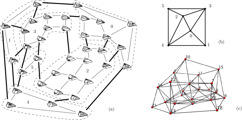
Figure 2: (a) The secondary polytope $\Sigma({\mathcal{A}})$ of two triangles (dark, light grey) and one segment $A_{0}=\{(0,0),(1,2),(4,1)\},\,A_{1}=\{(0,1),(1,0)\},\,A_{2}=\{(0,0),(0,1),(2,0)\}$, where ${\mathcal{A}}$ is defined as in Equation 1; vertices correspond to mixed subdivisions of the Minkowski sum $A_{0}+A_{1}+A_{2}$ and edges to flips between them (b) $N({\mathcal{R}})$, whose vertices correspond to the dashed classes of $\Sigma({\mathcal{A}})$. Bold edges of $\Sigma({\mathcal{A}})$, called cubical flips, map to edges of $N({\mathcal{R}})$ (c) $4$-dimensional $N({\mathcal{R}})$ of 3 generic trinomials with f-vector $(22,66,66,22)$; figure made with polymake.

Proposition 3 establishes a many-to-one surjection from regular triangulations of ${\mathcal{A}}$ to regular tight mixed subdivisions of $P$, or, equivalently, from vertices of $\Sigma({\mathcal{A}})$ to those of $N({\mathcal{R}})$. One defines an equivalence relationship on all regular tight mixed subdivisions, where equivalent subdivisions yield the same vertex in $N({\mathcal{R}})$. Thus, equivalent vertices of $\Sigma({\mathcal{A}})$ correspond to the same resultant vertex. Consider $w\in({\mathbb{R}}^{|{\mathcal{A}}|})^{\times}$ lying in the union of outer-normal cones of equivalent vertices of $\Sigma({\mathcal{A}})$. They correspond to a resultant vertex whose outer-normal cone contains $w$; this defines a $w$-extremal resultant monomial. If $w$ is non-generic, it specifies a sum of extremal monomials in ${\mathcal{R}}$, i.e. a face of $N({\mathcal{R}})$. The above discussion is illustrated in Figure 2(a),(b).

Proposition 4.

[Ref. 8] $N({\mathcal{R}})$ is a Minkowski summand of $\Sigma({\mathcal{A}})$, and both $\Sigma({\mathcal{A}})$ and $N({\mathcal{R}})$ have dimension $|{\mathcal{A}}|-2n-1.$

Let us describe the $2n+1$ hyperplanes in whose intersection lies $N({\mathcal{R}})$. For this, let $M$ be the $(2n+1)\times|{\mathcal{A}}|$ matrix whose columns are the points in the $A_{i}$, where each $a\in A_{i}$ is followed by the $i$-th unit vector in ${\mathbb{N}}^{n+1}$. Then, the inner product of any coordinate vector of $N({\mathcal{R}})$ with row $i$ of $M$ is: constant, for $i=1,\dots,n$, and known, and depends on $i$, for $i=n+1,\dots,2n+1$, see Prop. 7.1.11 of Ref. 8. This implies that one obtains an isomorphic polytope when projecting $N({\mathcal{R}})$ along $2n+1$ points in ${\mathcal{A}}$ which affinely span ${\mathbb{R}}^{2n}$; this is possible because of the assumption of essential family. Having computed the projection, we obtain $N({\mathcal{R}})$ by computing the missing coordinates as the solution of a linear system: we write the aforementioned inner products as $M[X\,V]^{T}=C$, where $C$ is a known matrix and $[X\,V]^{T}$ is a transposed $(2n+1)\times u$ matrix, expressing the partition of the coordinates to unknown and known values, where $u$ is the number of $N({\mathcal{R}})$ vertices. If the first $2n+1$ columns of $M$ correspond to specialized coefficients, $M=[M_{1}\,M_{2}]$, where submatrix $M_{1}$ is of dimension $2n+1$ and invertible, hence $X=M_{1}^{-1}(C-M_{2}B)$.

We compute some orthogonal projection of $N({\mathcal{R}})$, denoted $\varPi$, in ${\mathbb{R}}^{m}$:

$$\pi:{\mathbb{R}}^{|{\mathcal{A}}|}\rightarrow{\mathbb{R}}^{m}:N({\mathcal{R}})\rightarrow\varPi,\;\,m\leq|{\mathcal{A}}|.$$

By reindexing, this is the subspace of the first $m$ coordinates, so$\pi(\rho)=(\rho_{1},\dots,\rho_{m})$. It is possible that none of the coefficients $c_{ij}$ is specialized, hence $m=|{\mathcal{A}}|$, $\pi$ is trivial, and $\varPi=N({\mathcal{R}})$. Assuming the specialized coefficients take sufficiently generic values, $\varPi$ is the Newton polytope of the corresponding specialization of ${\mathcal{R}}$. The following is used for preprocessing.

Lemma 1.

[Ref. 7 Lemma 3.20] If $a_{ij}\in A_{i}$ corresponds to a specialized coefficient of $f_{i}$, and lies in the convex hull of the other points in $A_{i}$ corresponding to specialized coefficients, then removing $a_{ij}$ from $A_{i}$ does not change the Newton polytope of the specialized resultant.

We focus on three applications. First, we interpolate the resultant in all coefficients, thus illustrating an alternative method for computing resultants.

Example 2.

Let $f_{0}=a_{2}x^{2}+a_{1}x+a_{0}$, $f_{1}=b_{1}x^{2}+b_{0}$, with supports $A_{0}=\{2,1,0\},A_{1}=\{1,0\}$. Their (Sylvester) resultant is a polynomial in $a_{2},a_{1},a_{0},$ $b_{1},b_{0}$. Our algorithm computes its Newton polytope with vertices $(0,2,0,1,1)$, $(0,0,2,2,0)$, $(2,0,0,0,2)$; it contains 4 lattice points, corresponding to 4 potential resultant monomials $a_{1}^{2}b_{1}b_{0},~{}a_{0}^{2}b_{1}^{2},~{}a_{2}a_{0}b_{1}b_{0},~{}a_{2}^{2}b_{0}^{2}$. Knowing these potential monomials, to interpolate the resultant, we need 4 points $(a_{0},a_{1},a_{2},b_{0},b_{1})$ for which the system $f_{0}=f_{1}=0$ has a solution. For computing these points we use the parameterization of resultants in Ref. 24, which yields: $a_{2}=(2t_{1}+t_{2})t_{3}^{2}t_{4}$, $a_{1}=(-2t_{1}-2t_{2})t_{3}t_{4}$, $a_{0}=t_{2}t_{4}$, $b_{1}=-t_{1}t_{3}^{2}t_{5}$, $b_{0}=t_{1}t_{5},$ where the $t_{i}$’s are parameters. We substitute these expressions to the monomials, evaluate at 4 sufficiently random $t_{i}$’s, and obtain a matrix whose kernel vector $(1,1,-2,1)$ yields ${\mathcal{R}}=a_{1}^{2}b_{1}b_{0}+a_{0}^{2}b_{1}^{2}-2a_{2}a_{0}b_{1}b_{0}+a_{2}^{2}b_{0}^{2}$.

Second, consider system solving by the rational univariate representation of roots ²⁵. Given $f_{1},\dots,f_{n}\in{\mathbb{C}}[x_{1},\dots,x_{n}]$, define an overconstrained system by adding $f_{0}=u_{0}+u_{1}x_{1}+\cdots+u_{n}x_{n}$ with symbolic $u_{i}$’s. Let coefficients $c_{ij},i\geq 1$, take specific values, and suppose that the roots of $f_{1}=\cdots=f_{n}=0$ are isolated, denoted $r_{i}=(r_{i1},\dots,r_{in})$. Then the $u$-resultant is ${\mathcal{R}}_{u}=a\,\prod_{r_{i}}(u_{0}+u_{1}r_{i1}+\cdots+u_{n}r_{in})^{m_{i}}$, $a\in{\mathbb{C}}^{*}$, where $m_{i}$ is the multiplicity of $r_{i}$. Computing ${\mathcal{R}}_{u}$ is the bottleneck; our method computes (a superset of) $N({\mathcal{R}}_{u})$.

Example 3.

Let $f_{1}=x_{1}^{2}+x_{2}^{2}-4$, $f_{2}=x_{1}-x_{2}+2$, and $f_{0}=u_{0}+u_{1}x_{1}+u_{2}x_{2}$. Our algorithm computes a polygon with vertices $\{(2,0,0),(0,2,0),(0,0,2)\}$, which contains $N({\mathcal{R}}_{u})=\mbox{CH}(\{(2,0,0),(1,1,0),(1,0,1),(0,1,1)\})$. The coefficient specialization is not generic, hence $N({\mathcal{R}}_{u})$ is strictly contained in the computed polygon. Proceeding as in Example 2, ${\mathcal{R}}_{u}=2u_{0}^{2}+4u_{0}u_{1}-4u_{0}u_{2}-8u_{1}u_{2}$, which factors as $2(u_{0}+2u_{1})(u_{0}-2u_{2})$.

The last application comes from geometric modeling, where $y_{i}=f_{i}(x)$, $i=0,\dots,n$, $x=(x_{1},\dots,x_{n})\in\Omega\subset{\mathbb{R}}^{n}$, defines a parametric hypersurface. Many applications require the equivalent implicit representation $F(y_{1},\dots,y_{n})=0$. This amounts to eliminating $x$, so it is crucial to compute the resultant when coefficients are specialized except the $y_{i}$’s. Our approach computes a polytope that contains the Newton polytope of $F$, thus reducing implicitization to interpolation ^{4, 1}. In particular, we compute the polytope of surface equations within $1$sec, assuming $\leq 100$ terms in parametric polynomials, which includes all common instances in geometric modeling.

  

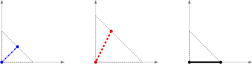
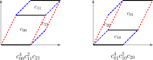
Figure 3: The supports $A_{0},A_{1},A_{2}$ of Example 4, their Newton polytopes (segments) and the two mixed subdivisions of their Minkowski sum.

Example 4.

Let us see how the above computation can serve in implicitization. Consider the surface given by the polynomial parameterization

$$(y_{1},y_{2},y_{3})=(x_{1}x_{2},x_{1}x_{2}^{2},x_{1}^{2}).$$

For polynomials $f_{0}:=c_{00}-c_{01}x_{1}x_{2},~{}f_{1}:=c_{10}-c_{11}x_{1}x_{2}^{2},~{}f_{2}:=c_{20}-c_{21}x_{1}^{2}$ with supports $A_{0}=\{(0,0),(1,2)\},A_{1}=\{(0,0),(1,2)\}$ and $A_{2}=\{(0,0),(2,0)\}$. The resultant polytope is a segment in ${\mathbb{R}}^{6}$ with endpoints $(4,0,0,2,0,1)$, $(0,4,2,0,1,0)$ and, actually, ${\mathcal{R}}=-c_{00}^{4}c_{11}^{2}c_{21}+c_{01}^{4}c_{10}^{2}c_{20}$. The supports and the two mixed subdivisions corresponding to the vertices of $N({\mathcal{R}})$ are illustrated in Figure 3. Specializing the symbolic coefficients of the polynomials as:

$$(c_{00},c_{01},c_{10},c_{11},c_{20},c_{21})\mapsto(y_{1},-1,y_{2},-1,y_{3},-1)$$

yields the vertices of the implicit polytope: $(4,0,0),(0,2,1)$, which our algorithm can compute directly. The implicit equation of the surface turns out to be $-y_{1}^{4}+y_{2}^{2}y_{3}$.

3 Algorithms and complexity

This section analyzes our exact and approximate algorithms for computing orthogonal projections of polytopes whose vertices are defined by an oracle. This oracle computes a vertex of the polytope which is extremal in a given direction $w$. If there are more than one such vertices the oracle returns exactly one of these. Moreover, we define such an oracle for the vertices of orthogonal projections $\varPi$ of $N({\mathcal{R}})$ which results in algorithms for computing $\varPi$ while avoiding computing $N({\mathcal{R}})$. Finally, we analyze the asymptotic complexity of these algorithms.

Given a pointset $V$, reg_subdivision($V,\omega$) computes the regular subdivision of its convex hull by projecting the upper hull of $V$ lifted by $\omega$, and conv($V$) computes the H-representation of the convex hull of $V$. The oracle VTX(${\mathcal{A}},\,w,\,\pi$) computes a point in $\varPi=\pi(N({\mathcal{R}}))$, extremal in the direction $w\in({\mathbb{R}}^{m})^{\times}$. First it adds to $w$ an infinitesimal symbolic perturbation vector, thus obtaining $w_{p}$. Then calls reg_subdivision(${\mathcal{A}},\widehat{w_{p}}$), $\widehat{w_{p}}=(w_{p},\vec{0})\in({\mathbb{R}}^{|{\mathcal{A}}|})^{\times}$ that yields a regular triangulation $T$ of ${\mathcal{A}}$, since $w_{p}$ is generic, and finally returns $\pi(\rho_{T})$. It is clear that the triangulation $T$ constructed by VTX$(\cdot)$ is regular and corresponds to some secondary vertex $\phi_{T}$ which maximizes the inner product with $\widehat{w_{p}}$. Since the perturbation is arbitrarily small, both $\phi_{T},\rho_{T}$ also maximize the inner product with $\widehat{w}=(w,\vec{0})\in({\mathbb{R}}^{|{\mathcal{A}}|})^{\times}$.

We use perturbation to avoid computing non-vertex points on the boundary of $\varPi$. The perturbation can be implemented in VTX$(\cdot)$, without affecting any other parts of the algorithm, either by case analysis or by a method of symbolic perturbation. In practice, our implementation does avoid computing non-vertex points on the boundary of $\varPi$ by computing a refinement of the subdivision obtained by calling reg_subdivision(${\mathcal{A}},\widehat{w}$). This refinement is implemented in triangulation by computing a placing triangulation with a random insertion order ²⁶ (Section 5).

Lemma 2.

All points computed by VTX$(\cdot)$ are vertices of $\varPi$.

Proof.

Let $v=\pi(\rho_{T})=\mbox{VTX}({\mathcal{A}},w,\pi)$. We first prove that $v$ lies on $\partial\varPi$. The point $\rho_{T}$ of $N({\mathcal{R}})$ is a Minkowski summand of the vertex $\phi_{T}$ of $\Sigma({\mathcal{A}})$ extremal with respect to $\widehat{w}$, hence $\rho_{T}$ is extremal with respect to $\widehat{w}$. Since $\widehat{w}$ is perpendicular to projection $\pi$, $\rho_{T}$ projects to a point in $\partial\varPi$. The same argument implies that every vertex $\phi_{T}^{\prime}$, where $T^{\prime}$ is a triangulation refining the subdivision produced by $\widehat{w}$, corresponds to a resultant vertex $\rho_{T^{\prime}}$ such that $\pi(\rho_{T^{\prime}})$ lies on a face of $\varPi$. This is actually the same face on which $\pi(\rho_{T})$ lies. Hence $\rho_{T^{\prime}}$ also lies on $\partial\varPi$.

Now we prove that $v$ is a vertex of $\varPi$ by showing that it does not lie in the relative interior of a face of $\Pi$. Let $w$ be such that the face $f$ of $N({\mathcal{R}})$ extremal with respect to $\widehat{w}$ contains a vertex $\rho_{T}$ which projects to $\mbox{relint}(\pi(f))$, where $\mbox{relint}(\cdot)$ denotes relative interior. However, $f$ will not be extremal with respect to $\widehat{w_{p}}$ and since VTX$({\mathcal{A}},w,\pi)$ uses the perturbed vector $w_{p}$, it will never compute a vertex of $N({\mathcal{R}})$ whose projection lies inside a face of $\varPi$. ∎

The initialization algorithm computes an inner approximation of $\varPi$ in both V- and H-representations (denoted $Q,\ Q^{H}$, respectively), and triangulated. First, it calls VTX$({\mathcal{A}},w,\pi)$ for $w\in W\subset({\mathbb{R}}^{m})^{\times}$; the set $W$ is either random or contains, say, vectors in the $2m$ coordinate directions. Then, it updates $Q$ by adding VTX$({\mathcal{A}},w,\pi)$ and VTX$({\mathcal{A}},-w,\pi)$, where $w$ is normal to hyperplane $H\subset{\mathbb{R}}^{m}$ containing $Q$, as long as either of these points lies outside $H$. Since every new vertex lies outside the affine hull of the current polytope $Q$, all polytopes produced are simplices. We stop when these points do no longer increase $\dim(Q)$.

Lemma 3.

The initialization algorithm computes $Q\subseteq\varPi$ such that $\dim(Q)=\dim(\varPi)$.

Proof.

Suppose that the initialization algorithm computes a polytope $Q^{\prime}\subset\varPi$ such that $\dim(Q^{\prime})<m$. Then there exists vertex $v\in\varPi$, $v\notin\mbox{Aff}(Q^{\prime})$ and vector $w\in({\mathbb{R}}^{m})^{\times}$ perpendicular to $\mbox{Aff}(Q^{\prime})$, such that $w$ belongs to the normal cone of $v$ in $\varPi$ and $\dim(\mbox{Aff}(Q^{\prime}\cup v))>\dim Q^{\prime}$. This is a contradiction, since such a $w$ would have been computed as VTX(${\mathcal{A}},w,\pi$) or VTX(${\mathcal{A}},-w,\pi$), where $w$ is normal to the hyperplane $H$ containing $Q^{\prime}$. ∎

Incremental Algorithm 1 computes both V- and H-representations of $\varPi$ and a triangulation of $\varPi$, given an inner approximation $Q,Q^{H}$ of $\varPi$ computed at the initialization. A hyperplane $H$ is called legal if it is a supporting hyperplane to a facet of $\varPi$, otherwise it is called illegal. At every step of Algorithm 1, we compute $v=\mbox{VTX}({\mathcal{A}},w,\pi)$ for a supporting hyperplane $H$ of a facet of $Q$ with normal $w$. If $v\notin H$, it is a new vertex thus yielding a tighter inner approximation of $\varPi$ by inserting it to $Q$, i.e. $Q\subset\mbox{CH}(Q\cup v)\subseteq\varPi$. This happens when the preimage $\pi^{-1}(f)\subset N({\mathcal{R}})$ of the facet $f$ of $Q$ defined by $H$, is not a Minkowski summand of a face of $\Sigma({\mathcal{A}})$ having normal $\widehat{w}$. Otherwise, there are two cases: either $v\in H$ and $v\in Q$, thus the algorithm simply decides hyperplane $H$ is legal, or $v\in H$ and $v\notin Q$, in which case the algorithm again decides $H$ is legal but also inserts $v$ to $Q$.

The algorithm computes $Q^{H}$ from $Q$, then iterates over the new hyperplanes to either compute new vertices or decide they are legal, until no increment is possible, which happens when all hyperplanes are legal. Algorithm 1 ensures that each normal $w$ to a hyperplane supporting a facet of $Q$ is used only once, by storing all used $w$’s in a set $W$. When a new normal $w$ is created, the algorithm checks if $w\notin W$, then calls VTX$({\mathcal{A}},w,\pi)$ and updates $W\leftarrow W\cup w$. If $w\in W$ then the same or a parallel hyperplane has been checked in a previous step of the algorithm. It is straightforward that $w$ can be safely ignored; Lemma 4 formalizes the latter case.

Lemma 4.

Let $H^{\prime}$ be a hyperplane supporting a facet constructed by Algorithm 1, and $H\neq H^{\prime}$ an illegal hyperplane at a previous step. If $H^{\prime},H$ are parallel then $H^{\prime}$ is legal.

Proof.

Let $w,w^{\prime}$ be the outer normal vectors of the facets supported by $H,H^{\prime}$ respectively. If $H,H^{\prime}$ are parallel then $v=\mbox{VTX}({\mathcal{A}},w,\pi)$ maximizes the inner product with $w^{\prime}$ in $Q$ which implies that hyperplane $H^{\prime}$ is legal. ∎

Input : essential $A_{0},\dots,A_{n}\subset{\mathbb{Z}}^{n}$ processed by Lemma 1,

projection $\pi:{\mathbb{R}}^{|{\mathcal{A}}|}\rightarrow{\mathbb{R}}^{m}$,

H-, V-repres. $Q^{H},Q$; triang. ${T}_{Q}$ of $Q\subseteq\varPi$.

Output : H-, V-repres. $Q^{H},Q$; triang. ${T}_{Q}$ of $Q=\varPi$.

${\mathcal{A}}\leftarrow\bigcup_{0}^{n}(A_{i}\times{e_{i}})$    // Cayley trick

${\cal H}_{illegal}\leftarrow\emptyset$;

foreach $H\in Q^{H}$ do ${\cal H}_{illegal}\leftarrow{\cal H}_{illegal}\cup\{H\}$      ;

while ${\cal H}_{illegal}\neq\emptyset$ do

       select $H\in{\cal H}_{illegal}$ and ${\cal H}_{illegal}\leftarrow{\cal H}_{illegal}\setminus\{H\}$;

       $w$ is the outer normal vector of $H$;

       $v\leftarrow$ VTX(${\mathcal{A}},w,\pi$);

       if $v\notin H\cap Q$ then

             $Q^{H}_{temp}\leftarrow{\rm conv}(Q\cup\{v\})$ // convex hull computation

             foreach $(d-1)$-face $f\in{T}_{Q}$ visible from $v$ do

                   ${T}_{Q}\leftarrow{T}_{Q}\cup\{\text{faces of }{conv}(f,v)\}$

            foreach $H^{\prime}\in\{Q^{H}\setminus Q^{H}_{temp}\}$ do

                   ${\cal H}_{illegal}\leftarrow{\cal H}_{illegal}\setminus\{H^{\prime}\}$ // $H^{\prime}$ separates $Q,v$

                  

            foreach $H^{\prime}\in\{Q^{H}_{temp}\setminus Q^{H}\}$ do

                   ${\cal H}_{illegal}\leftarrow{\cal H}_{illegal}\cup\{H^{\prime}\}$ // new hyperplane

                  

            $Q\leftarrow Q\cup\{v\}$;

             $Q^{H}\leftarrow Q^{H}_{temp}$;

            

      

return $Q,Q^{H},{T}_{Q}$;

Algorithm 1 Compute$\varPi$ $(A_{0},\dots,A_{n},\pi)$

The next lemma formulates the termination criterion of our algorithm.

Lemma 5.

Let $v=\mbox{{\em VTX}}({\mathcal{A}},w,\pi)$, where $w$ is normal to a supporting hyperplane $H$ of $Q$, then $v\not\in H$ if and only if $H$ is not a supporting hyperplane of $\varPi$.

Proof.

Let $v=\pi(\rho_{T})$, where $T$ is a triangulation refining subdivision $S$ in VTX$(\cdot)$. It is clear that, since $v\in\partial\varPi$ is extremal with respect to $w$, if $v\not\in H$ then $H$ cannot be a supporting hyperplane of $\varPi$. Conversely, let $v\in H$. By the proof of Lemma 2, every other vertex $\pi(\rho{{}_{T}^{\prime}})$ on the face of $N({\mathcal{R}})$ is extremal with respect to $w$, hence lies on $H$, thus $H$ is a supporting hyperplane of $\varPi$. ∎

We now bound the complexity of our algorithm. Beneath-and-Beyond, given a $k$-dimensional polytope with $l$ vertices, computes its H-representation and a triangulation in $O(k^{5}lt^{2})$, where $t$ is the number of full-dimensional faces (cells) Ref. 27. Let $|\varPi|,|\varPi^{H}|$ be the number of vertices and facets of $\varPi$.

Lemma 6.

Algorithm 1 executes VTX$(\cdot)$ at most $|\varPi|+|\varPi^{H}|$ times.

Proof.

The steps of Algorithm 1 increment $Q$. At every such step, and for each supporting hyperplane $H$ of $Q$ with normal $w$, the algorithm calls VTX$(\cdot)$ and computes one vertex of $\varPi$, by Lemma 2. If $H$ is illegal, this vertex is unique because $H$ separates the set of (already computed) vertices of $Q$ from the set of vertices of $\varPi\setminus Q$ which are extremal with respect to $w$, hence, an appropriate translate of $H$ also separates the corresponding sets of vertices of $\Sigma({\mathcal{A}})$ (Figure 4). This vertex is never computed again because it now belongs to $Q$. The number of VTX$(\cdot)$ calls yielding vertices is thus bounded by $|\varPi|$.

For a legal hyperplane of $Q$, we compute one vertex of $\varPi$ that confirms its legality; the VTX$(\cdot)$ call yielding this vertex is accounted for by the legal hyperplane. The statement follows by observing that every normal to a hyperplane of $Q$ is used only once in Algorithm 1 (by the earlier discussion concerning the set $W$ of all used normals). ∎

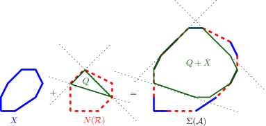
Figure 4: Lemma 6: each illegal hyperplane of $Q$ with normal $w$, separates the already computed vertices of $\varPi$ (here equal to $N({\mathcal{R}})$) from new ones, extremal with respect to $w$. $X$ is a polytope such that $X+N({\mathcal{R}})=\Sigma({\mathcal{A}})$.

Let the size of a triangulation be the number of its cells. Let $s_{{\mathcal{A}}}$ denote the size of the largest triangulation of ${\mathcal{A}}$ computed by VTX$(\cdot)$, and $s_{\varPi}$ that of $\varPi$ computed by Algorithm 1. In VTX$(\cdot)$, the computation of a regular triangulation reduces to a convex hull, computed in $O(n^{5}|{\mathcal{A}}|s_{{\mathcal{A}}}^{2})$; for $\rho_{{T}}$ we compute Volume for all cells of ${T}$ in $O(s_{{\mathcal{A}}}n^{3})$. The overall complexity of VTX$(\cdot)$ becomes $O(n^{5}|{\mathcal{A}}|s_{{\mathcal{A}}}^{2})$. Algorithm 1 calls, in every step, VTX$(\cdot)$ to find a point on $\partial\varPi$ and insert it to $Q$, or to conclude that a hyperplane is legal. By Lemma 6 it executes VTX$(\cdot)$ as many as $|\varPi|+|\varPi^{H}|$ times, in $O((|\varPi|+|\varPi^{H}|)n^{5}|{\mathcal{A}}|s_{{\mathcal{A}}}^{2})$, and computes the H-representation of $\varPi$ in $O(m^{5}|\varPi|s_{\varPi}^{2})$. Now we have, $|{\mathcal{A}}|\leq(2n+1)s_{{\mathcal{A}}}$ and as the input $|{\mathcal{A}}|,m,n$ grows large we can assume that $|\varPi|\gg|{\mathcal{A}}|$ and thus $s_{\varPi}$ dominates $s_{{\mathcal{A}}}$. Moreover, $s_{\varPi}(m+1)\geq|\varPi^{H}|$. Now, let $\widetilde{O}(\cdot)$ imply that polylogarithmic factors are ignored.

Theorem 1.

The time complexity of Algorithm 1 to compute $\varPi\subset{\mathbb{R}}^{m}$ is $O(m^{5}|\varPi|s_{\varPi}^{2}+(|\varPi|+|\varPi^{H}|)n^{5}|{\mathcal{A}}|s_{{\mathcal{A}}}^{2})$, which becomes $\widetilde{O}(|\varPi|s_{\varPi}^{2})$ when $|\varPi|\gg|{\mathcal{A}}|$.

This implies our algorithm is output sensitive. Its experimental performance confirms this property, see Section 5.

We have proven that oracle VTX$(\cdot)$ (within our algorithm) has two important properties:

1. Its output is a vertex of the target polytope (Lemma 2).

2. When the direction $w$ is normal to an illegal facet, then the vertex computed by the oracle is computed once (Lemma 6).
   

The algorithm can easily be generalized to incrementally compute any polytope $P$ if the oracle associated with the problem satisfies property (1); if it satisfies also property (2), then the computation can be done in $O(|P|+|P^{H}|)$ oracle calls, where $|P|$, $|P^{H}|$ denotes the number of vertices and number of facets of $P$, respectively. For example, if the described oracle returns $\pi(\phi_{T})$ instead of $\pi(\rho_{T})$, it can be used to compute orthogonal projections of secondary polytopes.

The algorithm readily yields an approximate variant: for each supporting hyperplane $H$, we use its normal $w$ to compute $v=$VTX$({\mathcal{A}},w,\pi)$. Instead of computing a convex hull, now simply take the hyperplane parallel to $H$ through $v$. The set of these hyperplanes defines a polytope $Q_{o}\supseteq\varPi$, i.e. an outer approximation of $\varPi$. In particular, at every step of the algorithm, $Q$ and $Q_{o}$ are an inner and an outer approximation of $\varPi$, respectively. Thus, we have an approximation algorithm by stopping Algorithm 1 when $\text{vol}(Q)/\text{vol}(Q_{o})$ achieves a user-defined threshold. Then, $\text{vol}(Q)/\text{vol}(\varPi)$ is bounded by the same threshold. Implementing this algorithm yields a speedup of up to 25 times (Section 5). It is clear that vol$(Q)$ is available by our incremental convex hull algorithm. However, vol$(Q_{o})$ is the critical step; we plan to examine algorithms that update (exactly or approximately) this volume.

When all hyperplanes of $Q$ are checked, knowledge of legal hyperplanes accelerates subsequent computations of $Q^{H}$, although it does not affect its worst-case complexity. Specifically, it allows us to avoid checking legal facets against new vertices.

4 Hashing of Determinants

This section discusses methods to avoid duplication of computations by exploiting the nature of the determinants appearing in the inner loop of our algorithm. Our algorithm computes many regular triangulations, which are typically dominated by the computation of determinants. A similar technique, using dynamic determinant computations, is used to improve determinantal predicates in incremental convex hull computations ²⁸.

Consider the $2n\times|{\mathcal{A}}|$ matrix with the points of ${\mathcal{A}}$ as columns. Define $P$ as the extension of this matrix by adding lifting values $\widehat{w}$ as the last row. We use the Laplace (or cofactor) expansion along the last row for computing the determinant of the square submatrix formed by any $2n+1$ columns of $P$; without loss of generality, we assume these are the first $2n+1$ columns $a_{1},\ldots,a_{2n+1}$. Let $(1,\ldots,2n+1)\setminus i$ be the vector resulting from removing the $i$-th element from the vector $(1,\ldots,2n+1)$ and let $P_{(1,\ldots,2n+1)\setminus i}$ be the $(2n)\times(2n)$ matrix obtained from the $2n$ elements of the columns whose indices are in $(1,\ldots,2n+1)\setminus i$.

The Orientation predicate is the sign of the determinant of $P^{hom}_{(1,\ldots,2n+2)}$, constructed by columns $a_{1},\ldots,a_{2n+2}$ and adding $\vec{1}\in{\mathbb{R}}^{2n+2}$ as the last row. Computing a regular subdivision is a long sequence of such predicates, varying $a_{i}$’s on each step. We expand along the next-to-last row, which contains the lifting values, and compute the determinants $|P_{(1,\ldots,2n+2)\setminus i}|$ for $i\in\{1,\ldots,2n+2\}$. Another predicate is Volume, used by VTX$(\cdot)$. It equals the determinant of $P^{hom}_{(1,\ldots,2n+1)}$, constructed by columns $a_{1},\ldots,a_{2n+1}$ and replacing the last row of the matrix by $\vec{1}\in{\mathbb{R}}^{2n+1}$.

Example 5.

Consider the polynomials $f_{0}:=c_{00}-c_{01}x_{1}x_{2}+c_{02}x_{2}$, $f_{1}:=c_{10}-c_{11}x_{1}x_{2}^{2}+c_{12}x_{2}^{2}$ and $f_{2}:=c_{20}-c_{21}x_{1}^{2}+c_{22}x_{2}$ and the lifting vector $\widehat{w}$ yielding the matrix $P$.

$$P=\begin{tabular}[]{|m{.5mm} >{\centering}m{\w} >{\centering}m{\w} >{\centering}m{\w} >{\centering}m{\w} >{\centering}m{\w} >{\centering}m{\w} >{\centering}m{\w} >{\centering}m{\w} >{\centering}m{\w} m{.5mm}| l}\cline{1-1}\cr\cline{11-11}\cr&$0$\@add@centering&$0$\@add@centering&$0$\@add@centering&$1$\@add@centering&$1$\@add@centering&$2$\@add@centering&$0$\@add@centering&$0$\@add@centering&$0$\@add@centering&&\hbox{\multirowsetup \Big{\}} \text{\small support coordinates}}\\ &$0$\@add@centering&$0$\@add@centering&$0$\@add@centering&$1$\@add@centering&$2$\@add@centering&$0$\@add@centering&$1$\@add@centering&$2$\@add@centering&$1$\@add@centering&\\ &\color[rgb]{1,0.49,0} $0$\@add@centering&\color[rgb]{1,0.49,0} $1$\@add@centering&\color[rgb]{1,0.49,0}$0$\@add@centering&\color[rgb]{1,0.49,0}$0$\@add@centering&\color[rgb]{1,0.49,0}$1$\@add@centering&\color[rgb]{1,0.49,0} $0$\@add@centering&\color[rgb]{1,0.49,0}$0$\@add@centering&\color[rgb]{1,0.49,0}$1$\@add@centering&\color[rgb]{1,0.49,0}$0$\@add@centering&&\hbox{\multirowsetup \Big{\}} \text{\small Cayley trick coordinates}}\\ &\color[rgb]{1,0.49,0}$0$\@add@centering&\color[rgb]{1,0.49,0}$0$\@add@centering&\color[rgb]{1,0.49,0}$1$\@add@centering&\color[rgb]{1,0.49,0}$0$\@add@centering&\color[rgb]{1,0.49,0}$0$\@add@centering&\color[rgb]{1,0.49,0}$1$\@add@centering&\color[rgb]{1,0.49,0}$0$\@add@centering&\color[rgb]{1,0.49,0}$0$\@add@centering&\color[rgb]{1,0.49,0}$1$\@add@centering&\\ &\color[rgb]{0,0.44,0.57}$w_{1}$\@add@centering&\color[rgb]{0,0.44,0.57}$w_{2}$\@add@centering&\color[rgb]{0,0.44,0.57}$w_{3}$\@add@centering&\color[rgb]{0,0.44,0.57}$0$\@add@centering&\color[rgb]{0,0.44,0.57}$0$\@add@centering&\color[rgb]{0,0.44,0.57}$0$\@add@centering&\color[rgb]{0,0.44,0.57}$0$\@add@centering&\color[rgb]{0,0.44,0.57}$0$\@add@centering&\color[rgb]{0,0.44,0.57}$0$\@add@centering&&\hbox{\multirowsetup \} \text{\small$\widehat{w}$}}\\ \cline{1-1}\cr\cline{11-11}\cr\end{tabular}$$

We reduce the computations of predicates to computations of minors of the matrix obtained from deleting the last row of $P$. Computing an Orientation predicate using Laplace expansion consists of computing $\binom{6}{4}=15$ minors. On the other hand, if we compute $|P^{hom}_{(1,2,3,4,5,6)}|$, the computation of $|P^{hom}_{(1,2,3,4,5,7)}|$ requires the computation of only $\binom{6}{4}-\binom{5}{4}=10$ new minors. More interestingly, when given a new lifting $\widehat{w^{\prime}}$, we compute $|P^{\prime}~{}^{hom}_{(1,2,3,4,5,6)}|$ without computing any new minors.

Our contribution consists in maintaining a hash table with the computed minors, which will be reused at subsequent steps of the algorithm. We store all minors of sizes between $2$ and $2n$. For Orientation, they are independent of $w$ and once computed they are stored in the hash table. The main advantage of our scheme is that, for a new ${w}$, the only change in $P$ are $m$ (nonzero) coordinates in the last row, hence computing the new determinants can be done by reusing hashed minors. This also saves time from matrix constructions.

Laplace expansion computation of a matrix of size $n$ has complexity$O(n)\sum_{i=1}^{n}L_{i}$, where $L_{i}$ is the cost of computing the $i$-th minor. $L_{i}$ equals $1$ when the $i$-th minor was precomputed; otherwise, it is bounded by $O\big{(}(n-1)!\big{)}$. This allows us to formulate the following Lemma.

Lemma 7.

Using hashing of determinants, the complexity of the Orientation and Volume predicates is $O(n)$ and $O(1)$, respectively, if all minors have already been computed.

Many determinant algorithms modify the input matrix; this makes necessary to create a new matrix and introduces a constant overhead on each minor computation. Computing with Laplace expansion, while hashing the minors of smaller size, performs better than state-of-the-art algorithms, in practice. Experiments in Section 5 show that our algorithm with hashed determinants outperforms the version without hash. For $m=3$ and $m=4$, we experimentally observed that the speedup factor is between 18 and 100; Figure 6 illustrates the second case.

The drawback of hashing determinants is the amount of storage, which is in $O(n!)$. The hash table can be cleared at any moment to limit memory consumption, at the cost of dropping all previously computed minors. Finding a policy to clear the hash table according to the number of times each minor was used would decrease the memory consumption, while keeping running times low. Exploring different heuristics, such as using a LRU (least recently used) cache, to choose which minors to drop when freeing memory will be an interesting research subject.

It is possible to exploit the structure of the above $(2n)\times(2n)$ minor matrices. Let $M$ be such a matrix, with columns corresponding to points of $A_{0},\dots,A_{n}$. After column permutations, we split $M$ into four $n\times n$ submatrices $A,B,D,I$, where $I$ is the identity matrix and $D$ has at most one $1$ in each column. This follows from the fact that the bottom half of every column in $M$ has at most one $1$ and the last $n$ rows of $M$ contain at least one $1$ each, unless $\det M=0$, which is easily checked. Now, $\det M=\pm\det(B-AD)$, with $AD$ constructed in $O(n)$. Hence, the computation of $(2n)\times(2n)$ minors is asymptotically equal to computing an $n\times n$ determinant. This only decreases the constant within the asymptotic bound. A simple implementation of this idea is not faster than Laplace expansion in the dimensions that we currently focus. However, this idea should be valuable in higher dimensions.

5 Implementation and Experiments

We implemented Algorithm 1 in C++ to compute $\varPi$; our code can be obtained from

http://respol.sourceforge.net.

All timings shown in this section were obtained on an Intel Core i5-2400 $3.1$GHz, with $6$MB L2 cache and $8$GB RAM, running 64-bit Debian GNU/Linux.

Our implementation, respol, relies on CGAL, using mainly a preliminary version of package triangulation ²⁶, for both regular triangulations, as well as for the V- and H-representation of $\varPi$. As for hashing determinants, we looked for a hashing function, that takes as input a vector of integers and returns an integer, which minimizes collisions. We considered many different hash functions, including some variations of the well-known FNV hash ²⁹. We obtained the best results with the implementation of Boost Hash ³⁰, which shows fewer collisions than the other tested functions. We clear the hash table when it contains $10^{6}$ minors. This gives a good tradeoff between efficiency and memory consumption. Last column of Table 1 shows that the memory consumption of our algorithm is related to $|A|$ and $\dim(\varPi)$.

We start our experiments by comparing four state-of-the-art exact convex hull packages: triangulation implementing Ref. 31 and beneath-and-beyond (bb) in polymake ³²; double description implemented in cdd ³³; and lrs implementing reverse search ³⁴. We compute $\varPi$, actually extending the work in Ref. 35 for the new class of polytopes $\varPi$. The triangulation package was shown to be faster in computing Delaunay triangulations in $\leq 6$ dimensions ²⁶. The other three packages are run through polymake, where we have ignored the time to load the data. We test all packages in an offline version. We first compute the V-representation of $\varPi$ using our implementation and then we give this as an input to the convex hull packages that compute the H-representation of $\varPi$. Moreover, we test triangulation by inserting points in the order that Algorithm 1 computes them, while improving the point location of these points since we know by the execution of Algorithm 1 one facet to be removed (online version). The experiments show that triangulation and bb are faster than lrs, which outperforms cdd. Furthermore, the online version of triangulation is $2.5$ times faster than its offline counterpart due to faster point location (Table 1, Figure 5).

$m$	$|{\mathcal{A}}|$	# of $\varPi$	time (seconds)						respol
		vertices	respol	tr/on	tr/off	bb	cdd	lrs	Mb
3	2490	318	85.03	0.07	0.10	0.07	1.20	0.10	37
4	27	830	15.92	0.71	1.08	0.50	26.85	3.12	46
4	37	2852	97.82	2.85	3.91	2.29	335.23	39.41	64
5	15	510	11.25	2.31	5.57	1.22	47.87	6.65	44
5	18	2584	102.46	13.31	34.25	9.58	2332.63	215.22	88
5	24	35768	4610.31	238.76	577.47	339.05	$>1$hr	$>1$hr	360
6	15	985	102.62	20.51	61.56	28.22	610.39	146.83	2868
6	19	23066	6556.42	1191.80	2754.30	$>1$hr	$>1$hr	$>1$hr	6693
7	12	249	18.12	7.55	23.95	4.99	6.09	11.95	114
7	17	500	302.61	267.01	614.34	603.12	10495.14	358.79	5258

Table 1: Total time and memory consumption of our code (respol) and time comparison of online version of triangulation (tr/on) and offline versions of all convex hull packages for computing the H-representation of $\varPi$.

Figure 5: Comparison of convex hull packages for $4$-dimensional (a) and $5$-dimensional (b) $\varPi$. triang_on/triang_off are the online/offline versions of triangulation package (y-axis is in logarithmic scale).

A placing triangulation of a set of points is a triangulation produced by the Beneath-and-Beyond convex hull algorithm for some ordering of the points. That is, the algorithm places the points in the triangulation with respect to the ordering. Each point which is going to be placed, is connected to all visible faces of the current triangulation resulting to the construction of new cells. An advantage of triangulation is that it maintains a placing triangulation of a polytope in ${\mathbb{R}}^{d}$ by storing the $0,1,d-1,d$-dimensional cells of the triangulation. This is useful when the oracle VTX$({\mathcal{A}},w,\pi)$ needs to refine the regular subdivision of ${\mathcal{A}}$ which is obtained by projecting the upper hull of the lifted pointset ${\mathcal{A}}^{\widehat{w}}$ (Section 3). In fact this refinement is attained by a placing triangulation, i.e., by computing the projection of the upper hull of the placing triangulation of ${\mathcal{A}}^{\widehat{w}}$. This is implemented in two steps:

1. compute the placing triangulation $T_{0}$ of the last $|{\mathcal{A}}|-m$ points with a random insertion order as described in Ref. 26 (they all have height zero),

2. place the first $m$ points of ${\mathcal{A}}^{\widehat{w}}$ in $T_{0}$ with a random insertion order ²⁶.

Step 1 is performed only once at the beginning of the algorithm, whereas Step 2 is performed every time we check a new $w$. The order of placing the points in Step 2 only matters if $w$ is not generic; otherwise, $w$ already produces a triangulation of the $m$ points, so any placing order results in this triangulation.

This is the implemented method; although different from the perturbation in the proof of Lemma 2, it is more efficient because of the reuse of triangulation $T_{0}$ in Step 1 above. Moreover, our experiments show that it always validates the two conditions in Section 3.

We can formulate this 2-step construction using a single lifting. Let $c>0$ be a sufficiently large constant, $a_{i}\in{\mathcal{A}},\,q_{i}\in{\mathbb{R}}$, $q_{i}>c\,q_{i+1},$ for $i=1,\ldots,|{\mathcal{A}}|$. Define lifting $h:{\mathcal{A}}\rightarrow{\mathbb{R}}^{2}$, where $h(a_{i})=(w_{i},q_{i}),$ for $i=1,\ldots,m$, and $h(a_{i})=(0,q_{i})$, for $i=m+1,\ldots,|{\mathcal{A}}|$. Then, projecting the upper hull of ${\mathcal{A}}^{h}$ to ${\mathbb{R}}^{2n}$ yields the triangulation of ${\mathcal{A}}$ obtained by the 2-step construction.

Fixing the dimension of the triangulation at compile time results in $<1\%$ speedup. We also tested a kernel that uses the filtering technique based on interval arithmetic from Ref. 36 with a similar time speedup. On the other hand, triangulation is expected to implement incremental high-dimensional regular triangulations with respect to a lifting, faster than the above method ³⁷. Moreover, we use a modified version of triangulation in order to benefit from our hashing scheme. Therefore, all cells of the triangulated facets of $\varPi$ have the same normal vector and we use a structure (STL set) to maintain the set of unique normal vectors, thus computing only one regular triangulation per triangulated facet of $\varPi$.

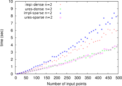
Figure 6: (a) Implicitization and $u$-resultants for $n=2,m=3$; (b) Comparison of respol (hashing and not hashing determinants) and Gfan (traversing tropical resultants and computing normal fan from stable intersection) for $m=4$; (c) Performance of Alg. 1 for $m=3,4,5$ as a function of input; (d) Performance of Alg. 1 as a function of its output; y-axes in (b), (c), (d) are in logarithmic scale.

We perform an experimental analysis of our algorithm. We design experiments parameterized on: the total number of input points $|{\mathcal{A}}|$, the dimension $n$ of pointsets $A_{i}$, and the dimension of projection $m$. First, we examine our algorithm on random inputs for implicitization and $u$-resultants, where $m=n+1$, while varying $|{\mathcal{A}}|,n$. We fix $\delta\in{\mathbb{N}}$ and select random points on the $\delta$-simplex to generate dense inputs, and points on the $(\delta/2)$-cube to generate sparse inputs. For implicitization the projection coordinates correspond to point $a_{i1}=(0,\ldots,0)\in A_{i}$. For $n=2$ the problem corresponds to implicitizing surfaces: when $|{\mathcal{A}}|<60$, we compute the polytopes in $<1$sec (Figure 6). When computing the $u$-resultant polytope, the projection coordinates correspond to $A_{0}=\{(1,\ldots,0),\ldots,(0,\dots,1)\}$. For $n=2$, when $|{\mathcal{A}}|<500$, we compute the polytopes in $<1$sec (Figure 6).

By using the hashing determinants scheme we gain a $18\times$ speedup when $n=2,\ m=3$. For $m=4$ we gain a larger speedup; we computed in $<2$min an instance where $|{\mathcal{A}}|=37$ and would take $>1$hr to compute otherwise. Thus, when the dimension and $|{\mathcal{A}}|$ becomes larger, this method allows our algorithm to compute instances of the problem that would be intractable otherwise, as shown for $n=3,\ m=4$ (Figure 6).

We confirm experimentally the output-sensitivity of our algorithm. First, our algorithm always computes vertices of $\varPi$ either to extend $\varPi$ or to legalize a facet. We experimentally show that our algorithm has, for fixed $m$, a subexponential behaviour with respect to both input and output (Figure 6, 6) and its output is subexponential with respect to the input.

# cells in triangulation				time (sec)				f-vector of $\varPi$
$\mu$	$\sigma$	min	max	$\mu$	$\sigma$	min	max
4781	154	4560	5087	0.35	0.01	0.34	0.38			449	1405	1438	482
16966	407	16223	17598	1.51	0.03	1.45	1.56			1412	4498	4705	1619
18229	935	16668	20058	1.92	0.10	1.77	2.11		432	1974	3121	2082	505
563838	6325	548206	578873	99	1.62	93.84	103.07		9678	43569	71004	50170	13059
289847	15788	264473	318976	69	4.88	61.67	77.31	1308	7576	16137	16324	7959	1504
400552	14424	374149	426476	96.5	4.91	88.86	107.12	1680	9740	21022	21719	10890	2133

Table 2: Typical f-vectors of projections of resultant polytopes and the size of their triangulations. We perform 20 runs with random insertion order of vertices for each polytope and report the minimum, maximum, average value $\mu$ and the standard deviation $\sigma$ for the number of cells and the runtime.

Figure 7: (a) $\mbox{vol}(Q)/\mbox{vol}(\varPi)$ as a function of the number of random normal vectors used to compute $Q$; (b) The size of the triangulation of $\varPi$ as a function of the output of Alg. 1.

As the complexity analysis (Theorem 1) indicates, the runtime of the algorithm depends on the size of the constructed placing triangulation of $\varPi$. The size of the placing triangulation depends on the ordering of the inserted points. We perform experiments on the effect of the inserting order to the size of the triangulation as well as the running time of the computation of the triangulation (Table 2). These sizes as well as the runtimes vary in a very narrow range. Thus, the insertion order is not crucial in both the runtime and the space of our algorithm. Further experiments in $4$-dimensional $N(R)$ show that the size of the input bounds polynomially the size of the triangulation of the output (Figure 7) which explains the efficiency of our algorithm in this dimension.

We explore the limits of our implementation. By bounding runtime to $<2$hr, we compute instances of $5$-, $6$-, $7$-dimensional $\varPi$ with $35$K, $23$K, $500$ vertices, respectively (Table 1).

We also compare with the implementation of Ref. 7, which is based on Gfan library. They develop two algorithms to compute projections of $N({\mathcal{R}})$. Assuming ${\mathcal{R}}$ defines a hypersurface, their methods compute a union of (possibly overlapping) cones, along with their multiplicities, see Theorem 2.9 of Ref. 7. From this intermediate result they construct the normal cones to the resultant vertices.

examples in Ref. 7	a	b	c	d	e	f	g	h	i
$|{\mathcal{A}}|$	12	12	15	12	12	16	27	16	20
$m$	12	12	15	6	7	9	3	4	5
$n$	3	2	4	2	2	3	2	3	4
Gfan(secs∗)	1.40	6	55	0.70	1.30	798	0.40	2.60	184
respol(secs)	1.40	18.41	99.90	0.26	1.24	934	0.02	0.96	292.01

Table 3: Comparison of our implementation with Gfan. ^∗ Timings for Gfan as reported in Ref. 7.

We compare with the best timings of Gfan methods using the examples and timings of Ref. 7 (Table 3). Our method is faster in examples (d), (e), (g), (h) where $m<7$, is competitive (up to $2$ times slower) in (a) where $m=|{\mathcal{A}}|=12$ and (i) where $m=5,|{\mathcal{A}}|=20$ and slower in (b), (c), (f) where $m\geq 12$. The bottleneck of our implementation, that makes it slower when the dimension of the projection $m$ is high, is the incremental convex hull construction in ${\mathbb{R}}^{m}$. Moreover, since our implementation considers that $N({\mathcal{R}})$ lies in ${\mathbb{R}}^{|{\mathcal{A}}|}$ instead of ${\mathbb{R}}^{|{\mathcal{A}}|-2n-1}$, (see also the discussion on the homogeneities of ${\mathcal{R}}$ in Section 2), it cannot take advantage of the fact that $\dim(N({\mathcal{R}}))$ could be less than $m$ when $|{\mathcal{A}}|-2n-1<m<|{\mathcal{A}}|$. This is the case in examples (b), (c) and (f). On the other hand, we run extensive experiments for $n=3$, considering implicitization, where $m=4$ and our method, with and without using hashing, is much faster than any of the two algorithms based on Gfan (Figure 6). However, for $n=4,\ m=5$ the beta version of Gfan used in our experiments was not stable and always crashed when $|{\mathcal{A}}|>13$.

input		m	3	3	4	4	5	5
		$|{\mathcal{A}}|$	200	490	20	30	17	20
approximation		# of $Q$ vertices	15	11	63	121	$>10$hr	$>10$hr
		$\mbox{vol}(Q)/\mbox{vol}(\varPi)$	0.96	0.95	0.93	0.94	$>10$hr	$>10$hr
algorithm		$\mbox{vol}(Q_{o})/\mbox{vol}(\varPi)$	1.02	1.03	1.04	1.03	$>10$hr	$>10$hr
		time (sec)	0.15	0.22	0.37	1.42	$>10$hr	$>10$hr
uniformly		$|Q|$	34	45	123	207	228	257
		random vectors	606	576	613	646	977	924
random		$\mbox{vol}(Q)/\mbox{vol}(\varPi)$	0.93	0.99	0.94	0.90	0.90	0.90
		time (sec)	5.61	12.78	1.10	4.73	8.41	16.90
exact		# of $\varPi$ vertices	98	133	416	1296	1674	5093
algorithm		time (sec)	2.03	5.87	3.72	25.97	51.54	239.96

Table 4: Results on experiments computing $Q,Q_{o}^{H}$ using the approximation algorithm and the random vectors procedure; we stop the approximation algorithm when $\mbox{vol}(Q)/\mbox{vol}(Q_{o})>0.9$; the results with random vectors are the average values over $10$ independent experiments; “$>10$hr” indicates computation of $\mbox{vol}(Q_{o})$ was interrupted after $10$hr.

We analyze the computation of inner and outer approximations $Q$ and $Q_{o}^{H}$. We test the variant of Section 3 by stopping it when $\mbox{vol}(Q)/\mbox{vol}(Q_{o}^{H})>0.9$. In the experiments, the number of $Q$ vertices is $<15\%$ of the $\varPi$ vertices, thus there is a speedup of up to $25$ times over the exact algorithm at the largest instances. The approximation of the volume is very satisfactory: $\mbox{vol}(Q_{o}^{H})/\mbox{vol}(\varPi)<1.04$ and $\mbox{vol}(Q)/\mbox{vol}(\varPi)>0.93$ for the tested instances (Table 4). The bottleneck here is the computation of vol$(Q_{o}^{H})$, where $Q_{o}^{H}$ is given in H-representation: the runtime explodes for $m\geq 5$. We use polymake in every step to compute vol$(Q_{o}^{H})$ because we are lacking of an implementation that, given a polytope $P$ in H-representation, its volume and a halfspace $H$, computes the volume of the intersection of $P$ and $H$. Note that we do not include this computation time in the reported time. Our current work considers ways to extend these observations to a polynomial time approximation algorithm for the volume and the polytope itself when the latter is given by an optimization oracle, as is the case here.

Next, we study procedures that compute only the V-representation of $Q$. For this, we count how many random vectors uniformly distributed on the $m$-dimensional sphere are needed to obtain $\mbox{vol}(Q)/\mbox{vol}(\varPi)>0.9$. This procedure runs up to $10$ times faster than the exact algorithm (Table 4). Figure 7 illustrates the convergence of $\mbox{vol}(Q)/\mbox{vol}(\varPi)$ to the threshold value $0.9$ in typical $3,4,5$-dimensional examples. The basic drawback of this method is that it does not provide guarantees for $\mbox{vol}(Q)/\mbox{vol}(\varPi)$ because we do not have sufficient a priori information on $\varPi$. These experiments also illustrate the extent in which the normal vectors required to deterministically construct $\varPi$ are uniformly distributed over the sphere.

6 Future work

One algorithm that should be experimentally evaluated is the following. We perform a search over the vertices of $\Sigma(A)$, that is, we build a search tree with flips as edges. We keep a set with the extreme vertices with respect to a given projection. Each computed vertex that is not extreme in the above set is discarded and no flips are executed on it, i.e. the search tree is pruned in this vertex. The search procedure could be the algorithm of TOPCOM or the one presented in Ref. 14 which builds a search tree in some equivalence classes of $\Sigma(A)$. The main advantage of this algorithm is that it does not involve a convex hull computation. On the other hand, it is not output-sensitive with respect to the number of vertices of the resultant polytope; its complexity depends on the number of vertices on the silhouette of $\Sigma(A)$, with respect to a given projection and those that are connected by an edge with them.

As shown, polymake’s convex hull algorithm is competitive, thus one may use it for implementing our algorithm. On the other hand, triangulation is expected to include fast enumeration of all regular triangulations for a given (non generic) lifting, in which case $\varPi$ may be extended by more than one (coplanar) vertices.

Our proposed algorithm uses an incremental convex hull algorithm and it is known that any such algorithm has a worst-case super-polynomial total time complexity ³⁸ in the number of input points and output facets. The basic open question that this paper raises is whether there is a polynomial total time algorithm for $\varPi$ or even for the set of its vertices.

7 Acknowledgments

All authors were partially supported from project “Computational Geometric Learning”, which acknowledges the financial support of the Future and Emerging Technologies (FET) programme within the 7th Framework Programme for research of the European Commission, under FET-Open grant number: 255827. Most of the work was done while C. Konaxis and L. Peñaranda were at the University of Athens. C. Konaxis’ research leading to these results has also received funding from the European Union’s Seventh Framework Programme (FP7-REGPOT-2009-1) under grant agreement n^o 245749. We thank O. Devillers and S. Hornus for discussions on triangulation, and A. Jensen and J. Yu for discussions and for sending us a beta version of their code.

References

- [1] I.Z. Emiris, T. Kalinka, C. Konaxis, and T. Luu Ba. Implicitization of curves and (hyper)surfaces using predicted support. Theor. Comp. Science, Special Issue on Symbolic & Numeric Computing, 479(0):81–98, 2013.
- [2] B. Sturmfels and J. Yu. Tropical implicitization and mixed fiber polytopes. In Software for Algebraic Geometry, volume 148 of IMA Volumes in Math. & its Applic., pages 111–131. Springer, New York, 2008.
- [3] J. Rambau. TOPCOM: Triangulations of point configurations and oriented matroids. In Proc. Intern. Congress Math. Software, pages 330–340, 2002.
- [4] I.Z. Emiris, T. Kalinka, C. Konaxis, and T. Luu Ba. Sparse implicitization by interpolation: Characterizing non-exactness and an application to computing discriminants. J. Computer Aided Design, 45:252–261, 2013. Special Issue on Symposium Solid & Phys. Modeling 2012 (Dijon, France).
- [5] F. Rincón. Computing tropical linear spaces. In J. Symbolic Computation, volume 51, pages 86–98, 2013.
- [6] CGAL: Computational geometry algorithms library. http://www.cgal.org.
- [7] A. Jensen and J. Yu. Computing tropical resultants. arXiv:math.AG/1109.2368v1, 2011.
- [8] I.M. Gelfand, M.M. Kapranov, and A.V. Zelevinsky. Discriminants, Resultants and Multidimensional Determinants. Birkhäuser, Boston, 1994.
- [9] B. Sturmfels. On the Newton polytope of the resultant. J. Algebraic Combin., 3:207–236, 1994.
- [10] A. Dickenstein, I.Z. Emiris, and V. Fisikopoulos. Combinatorics of 4-dimensional resultant polytopes. In Proc. ACM Intern. Symp. on Symbolic & Algebraic Comput., 2013. (to appear).
- [11] S.Yu. Orevkov. The volume of the Newton polytope of a discriminant. Russ. Math. Surv., 54(5):1033–1034, 1999.
- [12] H. Imai, T. Masada, F. Takeuchi, and K. Imai. Enumerating triangulations in general dimensions. Intern. J. Comput. Geom. Appl., 12(6):455–480, 2002.
- [13] T. Michiels and R. Cools. Decomposing the secondary Cayley polytope. Discr. Comput. Geometry, 23:367–380, 2000.
- [14] T. Michiels and J. Verschelde. Enumerating regular mixed-cell configurations. Discr. Comput. Geometry, 21(4):569–579, 1999.
- [15] P. Huggins. ib4e: A software framework for parametrizing specialized lp problems. In A. Iglesias and N. Takayama, editors, Mathematical Software (ICMS 2006), volume 4151 of Lecture Notes in Computer Science, pages 245–247. Springer, Berlin, 2006.
- [16] E. Kaltofen and G. Villard. On the complexity of computing determinants. Computational Complexity, 13:91–130, 2005.
- [17] H. Brönnimann, I.Z. Emiris, V. Pan, and S. Pion. Sign determination in Residue Number Systems. Theor. Comp. Science, Spec. Issue on Real Numbers & Computers, 210(1):173–197, 1999.
- [18] J.-G. Dumas, T. Gautier, M. Giesbrecht, P. Giorgi, B. Hovinen, E. Kaltofen, B. D. Saunders, W. J. Turner, and G. Villard. Linbox: A generic library for exact linear algebra. In Proc. Intern. Congress Math. Software, pages 40–50, Beijing, 2002.
- [19] G. Guennebaud, B. Jacob, et al. Eigen v3. http://eigen.tuxfamily.org, 2010.
- [20] I.Z. Emiris, V. Fisikopoulos, C. Konaxis, and L. Peñaranda. An output-sensitive algorithm for computing projections of resultant polytopes. In Proc. Annual ACM Symp. Computational Geometry, pages 179–188, 2012.
- [21] J.A. De Loera, J. Rambau, and F. Santos. Triangulations: Structures for Algorithms and Applications, volume 25 of Algorithms and Computation in Mathematics. Springer, 2010.
- [22] G.M. Ziegler. Lectures on Polytopes. Springer, 1995.
- [23] D. Cox, J. Little, and D. O’Shea. Using Algebraic Geometry. Number 185 in GTM. Springer, New York, 2nd edition, 2005.
- [24] M.M. Kapranov. Characterization of A-discriminantal hypersurfaces in terms of logarithmic Gauss map. Math. Annalen, 290:277–285, 1991.
- [25] S. Basu, R. Pollack, and M.-F. Roy. Algorithms in real algebraic geometry. Springer-Verlag, Berlin, 2003.
- [26] J.-D. Boissonnat, O. Devillers, and S. Hornus. Incremental construction of the Delaunay triangulation and the Delaunay graph in medium dimension. In Proc. Annual ACM Symp. Computational Geometry, pages 208–216, 2009.
- [27] M. Joswig. Beneath-and-beyond revisited. In M. Joswig and N. Takayama, editors, Algebra, Geometry, and Software Systems, Mathematics and Visualization. Springer, Berlin, 2003.
- [28] V. Fisikopoulos and L. Peñaranda. Faster geometric algorithms via dynamic determinant computation. In Proc. 20th Europ. Symp. Algorithms, pages 443–454, 2012.
- [29] G. Fowler, L.C. Noll, and P. Vo. Fowler/Noll/Vo (FNV) hash algorithm. http://www.isthe.com/chongo/tech/comp/fnv, 1991.
- [30] D. James. Boost functional library. http://www.boost.org/libs/functional/hash, 2008.
- [31] K.L. Clarkson, K. Mehlhorn, and R. Seidel. Four results on randomized incremental constructions. Comput. Geom.: Theory & Appl., 3:185–121, 1993.
- [32] E. Gawrilow and M. Joswig. Polymake: an approach to modular software design in computational geometry. In Proc. Annual ACM Symp. Computational Geometry, pages 222–231. ACM Press, 2001.
- [33] K. Fukuda. cdd and cdd+ Home Page. ETH Z\a”urich. http://www.ifor.math.ethz.ch/~fukuda/cdd_home, 2008.
- [34] D. Avis. lrs: A revised implementation of the reverse search vertex enumeration algorithm. In Polytopes: Combinatorics & Computation, volume 29 of Oberwolfach Seminars, pages 177–198. Birkhäuser, 2000.
- [35] D. Avis, D. Bremner, and R. Seidel. How good are convex hull algorithms? Comput. Geom.: Theory & Appl., 7:265–301, 1997.
- [36] H. Brönnimann, C. Burnikel, and S. Pion. Interval arithmetic yields efficient dynamic filters for computational geometry. In Proc. Annual ACM Symp. Computational Geometry, pages 165–174, New York, 1998. ACM.
- [37] O. Devillers, 2011. Personal communication.
- [38] D. Bremner. Incremental convex hull algorithms are not output sensitive. In Proc. 7th Intern. Symp. Algorithms and Comput., pages 26–35, London, UK, 1996. Springer.