Estimating the number of zero-one multi-way tables via sequential importance sampling

Abstract.

In 2005, Chen et al introduced a sequential importance sampling (SIS) procedure to analyze zero-one two-way tables with given fixed marginal sums (row and column sums) via the conditional Poisson (CP) distribution. They showed that compared with Monte Carlo Markov chain (MCMC)-based approaches, their importance sampling method is more efficient in terms of running time and also provides an easy and accurate estimate of the total number of contingency tables with fixed marginal sums. In this paper we extend their result to zero-one multi-way ($d$-way, $d\geq 2$) contingency tables under the no $d$-way interaction model, i.e., with fixed $d-1$ marginal sums. Also we show by simulations that the SIS procedure with CP distribution to estimate the number of zero-one three-way tables under the no three-way interaction model given marginal sums works very well even with some rejections. We also applied our method to Samson’s monks’ data set. We end with further questions on the SIS procedure on zero-one multi-way tables.

1. Introduction

Sampling zero-one constrained contingency tables finds its applications in combinatorics [7], statistics of social networks [2, 9], and regulatory networks [6]. In 2005, Chen et al. introduced a sequential importance sampling (SIS) procedure to analyze zero-one two-way tables with given fixed marginal sums (row and column sums) via the conditional Poisson (CP) distribution [3]. It proceeds by simply sampling cell entries of the zero-one contingency table sequentially for each row such that the final distribution approximates the target distribution. This method will terminate at the last column and sample independently and identically distributed (iid) tables from the proposal distribution. Thus the SIS procedure does not require expensive or prohibitive pre-computations, as is the case of computing Markov bases for the Monte Carlo Markov Chain (MCMC) approach. Also, when attempting to sample a single table, if there is no rejection, the SIS procedure is guaranteed to sample a table from the distribution, where in an MCMC approach the chain may require a long time to run in order to satisfy the independent condition.

In 2007, Chen extended their SIS procedure to sample zero-one two-way tables with given fixed row and column sums with structural zeros, i.e., some cells are constrained to be zero or one [2]. In this paper we also extended the results from [3, 2] to zero-one multi-way ($d$-way, $d\geq 2$) contingency tables under the no $d$-way interaction model, i.e., with fixed $d-1$ marginal sums.

This paper is organized as follows: In Section 2 we outline basics of the SIS procedure. In Section 3 we focus on the SIS procedure with CP distribution on three-way tables under no three-way interaction model. This model is particularly important since if we are able to count or estimate the number of tables under this model then this is equivalent to estimating the number of lattice points in any polytope [4]. This means that if we can estimate the number of three-way zero-one tables under this model, then we can estimate the number of any zero-one tables by using De Loera and Onn’s bijection mapping.

Let $\mathchoice{\mbox{\boldmath$\displaystyle\bf X$}}{\mbox{\boldmath$\textstyle\bf X$}}{\mbox{\boldmath$\scriptstyle\bf X$}}{\mbox{\boldmath$\scriptscriptstyle\bf X$}}=(X_{ijk})$ of size $(m\mbox{, }n\mbox{, }l)$, where $m,n,l\in{\mathbb{N}}$ and ${\mathbb{N}}=\{1,2,\ldots,\}$, be a table of counts whose entries are independent Poisson random variables with canonical parameters $\{\theta_{ijk}\}$. Here $X_{ijk}\in\{0,1\}$. Consider the generalized linear model,

(1.1) $$\theta_{ijk}=\lambda+\lambda^{M}_{i}+\lambda^{N}_{j}+\lambda^{L}_{k}+\lambda_{ij}^{MN}+\lambda_{ik}^{ML}+\lambda_{jk}^{NL}\,$$

for $i=1,\ldots,m$, $j=1,\ldots,n$, and $k=1,\ldots,l$ where $M$, $N$, and $L$ denote the nominal-scale factors. This model is called the no three-way interaction model.

Notice that the sufficient statistics under the model in (1.1) are the two-way marginals, that is:

(1.2) $$\begin{array}[]{ll}X_{+jk}:=\sum_{i=1}^{m}X_{ijk}\mbox{, }(j=1,2,\ldots,n\mbox{, }k=1,2,\ldots,l),\\ X_{i+k}:=\sum_{j=1}^{n}X_{ijk}\mbox{, }(i=1,2,\ldots,m\mbox{, }k=1,2,\ldots,l),\\ X_{ij+}:=\sum_{k=1}^{l}X_{ijk}\mbox{, }(i=1,2,\ldots,m\mbox{, }j=1,2,\ldots,n),\\ \end{array}$$

Hence, the conditional distribution of the table counts given the margins is the same regardless of the values of the parameters in the model.

In Section 4 we generalize the SIS procedure on zero-one two-way tables in [3, 2] to zero-one multi-way ($d$-way, $d\geq 2$) contingency tables under the no $d$-way interaction model, i.e., with fixed $d-1$ marginal sums. In Sections 5 and 6 we show some simulation results with our software which is available in http://www.polytopes.net/code/CP. Finally, we end with some discussions.

2. Sequential importance sampling

Let $\Sigma$ be the set of all tables satisfying marginal conditions. In this paper we assume that $\Sigma\not=\emptyset$. Let $P({\bf X})$ for any ${\bf X}\in\Sigma$ be the uniform distribution over $\Sigma$, so $p({\bf X})=1/|\Sigma|$. Let $q(\cdot)$ be a trial distribution such that $q({\bf X})>0$ for all ${\bf X}\in\Sigma$. Then we have

$${\mathbb{E}}\left[\frac{1}{q({\bf X})}\right]=\sum_{{\bf X}\in\Sigma}\frac{1}{q({\bf X})}q({\bf X})=|\Sigma|.$$

Thus we can estimate $|\Sigma|$ by

$$\widehat{|\Sigma|}=\frac{1}{N}\sum_{i=1}^{N}\frac{1}{q({\bf X_{i}})},$$

where ${\bf X_{1}},\ldots,{\bf X_{N}}$ are tables drawn iid from $q({\bf X})$. Here, this proposed distribution $q({\bf X})$ is the distribution (approximate) to sample tables via the SIS procedure.

We vectorized the table ${\bf X}=(x_{1},\cdots,x_{t})$ and by the multiplication rule we have

$$q({\bf X}=(x_{1},\cdots,x_{t}))=q(x_{1})q(x_{2}|x_{1})q(x_{3}|x_{2},x_{1})\cdots q(x_{t}|x_{t-1},\ldots,x_{1}).$$

Since we sample each cell count of a table from an interval we can easily compute $q(x_{i}|x_{i-1},\ldots,x_{1})$ for $i=2,3,\ldots,t$.

When we have rejections, this means that we are sampling tables from a bigger set $\Sigma^{*}$ such that $\Sigma\subset\Sigma^{*}$. In this case, as long as the conditional probability $q(x_{i}|x_{i-1},\ldots,x_{1})$ for $i=2,3,\ldots$ and $q(x_{1})$ are normalized, $q({\bf X})$ is normalized over $\Sigma^{*}$ since

$$\begin{array}[]{rcl}\sum_{{\bf X}\in\Sigma^{*}}q({\bf X})&=&\sum_{x_{1},\ldots,x_{t}}q(x_{1})q(x_{2}|x_{1})q(x_{3}|x_{2},x_{1})\cdots q(x_{t}|x_{t-1},\ldots,x_{1})\\ &=&\sum_{x_{1}}q(x_{1})\left[\sum_{x_{2}}q(x_{1}|x_{2})\left[\cdots\left[\sum_{x_{t}}q(x_{t}|x_{t-1},\ldots,x_{1})\right]\right]\right]\\ &=&1.\\ \end{array}$$

Thus we have

$${\mathbb{E}}\left[\frac{\mathbb{I}_{{\bf X}\in\Sigma}}{q({\bf X})}\right]=\sum_{{\bf X}\in\Sigma^{*}}\frac{\mathbb{I}_{{\bf X}\in\Sigma}}{q({\bf X})}q({\bf X})=|\Sigma|,$$

where $\mathbb{I}_{{\bf X}\in\Sigma}$ is an indicator function for the set $\Sigma$. By the law of large numbers this estimator is unbiased.

3. Sampling from the conditional Poisson distribution

Let

$$Z=(Z_{1},\ldots,Z_{l})$$

be independent Bernoulli trials with probability of successes $p=(p_{1},\ldots,p_{l})$. Then the random variable

$$S_{Z}=Z_{1}+\cdots+Z_{l}$$

is a Poisson–binomial distribution.

We say the column of entries for the marginal $X_{i_{0},j_{0},+}$ of $\textstyle\bf X$ is the $(i_{0},j_{0})$th column of $\textstyle\bf X$ (equivalently we say $(i_{0},k_{0})$th column for the marginal $X_{i_{0}+k_{0}}$ and $(j_{0},k_{0})$th column for the marginal $X_{+j_{0}k_{0}}$). Consider the $(i_{0},j_{0})$th column of the table $\textstyle\bf X$ for some $i_{0}\in\{1,\ldots,m\}$, $j_{0}\in\{1,\ldots,n\}$ with the marginal $l_{0}=X_{i_{0}j_{0}+}$. Also we let $r_{k}=X_{i_{0}+k}$ and $c_{k}=X_{+j_{o}k}$. Now let $w_{k}=p_{k}/(1-p_{k})$ where $p_{k}\in(0,\,1)$. Then,

(3.1) $$P(Z_{1}=z_{1},\ldots,Z_{l}=z_{l}|S_{Z}=l_{0})\propto\prod_{k=1}^{l}w_{k}^{z_{k}}.$$

Thus for sampling a zero-one table with fixed marginals $X_{+jk},\,X_{i+k}$ for $i=1,2,\ldots,m\mbox{, }j=1,2,\ldots,n$, and $k=1,2,\ldots,l$, for $X_{i_{0}j_{0}+}$ for each $i_{0}\in\{1,\ldots,m\}$ and $j_{0}\in\{1,\ldots,n\}$, (or one can do each $X_{i_{0}+k_{0}}$ or $X_{+j_{0}k_{0}}$ instead by similar way) one just decides which entries are ones (basically there are ${l\choose l_{0}}$ many choices) using the conditional Poisson distribution above. We sample these cell entries with ones (say $l_{0}$ many entries with ones) in the $(i_{0},j_{0})$th column for the $L$ factor with the following probability: Let $A_{k}$, for $k=1,\ldots,l_{0}$, be the set of selected entries. Thus $A_{0}=\emptyset$, and $A_{l_{0}}$ is the final sample that we obtain. At the $k$th step of the drafting sampling $(k=1,\ldots,l_{0})$, a unit $j\in A^{c}_{k-1}$ is selected into the sample with probability

$$P(j,A^{c}_{k-1})=\frac{w_{j}R(l_{0}-k,A^{c}_{k-1}-j)}{(l_{0}-k+1)R(l_{0}-k+1,A^{c}_{k-1})},$$

where

$$R(s,A)=\sum_{B\subset A,|B|=s}\left(\prod_{i\in B}w_{i}\right).$$

For sampling a zero-one three-way table $\textstyle\bf X$ with given two-way marginals $X_{ij+}$, $X_{i+k}$, and $X_{+jk}$ for $i=1,2,\ldots,m\mbox{, }j=1,2,\ldots,n$, and $k=1,2,\ldots,l$, we sample for the $(i_{0},j_{0})$th column of the table $\textstyle\bf X$ for each $i_{0}\in\{1,\ldots,m\}$, $j_{0}\in\{1,\ldots,n\}$. We set

(3.2) $$p_{k}:=\frac{r_{k}\cdot c_{k}}{r_{k}\cdot c_{k}+(n-r_{k})(m-c_{k})}.$$

Thus we have

(3.3) $$w_{k}=\frac{r_{k}\cdot c_{k}}{(n-r_{k})(m-c_{k})}.$$

Remark 3.1.

We assume that we do not have the trivial cases, namely, $1\leq r_{k}\leq n-1$ and $1\leq c_{k}\leq m-1$.

Theorem 3.2.

For the uniform distribution over all $m\times n\times l$ zero-one tables with given marginals $r_{k}=X_{i_{0}+k},\,c_{k}=X_{+j_{0}k}$ for $k=1,2,\ldots,l$, and a fixed marginal for the factor $L$, $l_{0}$, the marginal distribution of the fixed marginal $l_{0}$ is the same as the conditional distribution of $Z$ defined by (3.1) given $S_{Z}=l_{0}$ with

$$p_{k}:=\frac{r_{k}\cdot c_{k}}{r_{k}\cdot c_{k}+(n-r_{k})(m-c_{k})}.$$

Proof.

We start by giving an algorithm for generating tables uniformly from all $m\times n\times l$ zero-one tables with given marginals $r_{k},\,c_{k}$ for $k=1,2,\ldots,l$, and a fixed marginal for the factor $L$, $l_{0}$.

1. For $k=1,\ldots,l$ consider the $k$th layer of $m\times n$ tables. We randomly choose $r_{k}$ positions in the $(i_{0},k)$th column and $c_{k}$ positions in the $(j_{0},k)$th column, and put $1$’s in those positions. The choices of positions are independent across different layers.

2. Accept those tables with given column sum $l_{0}$.

It is easy to see that tables generated by this algorithm are uniformly distributed over all $m\times n\times l$ zero-one tables with given marginals $r_{k},\,c_{k}$ for $k=1,2,\ldots,l$, and a fixed marginal for the factor $L$, $l_{0}$ for the $(i_{0},j_{0})$th column of the table $\textstyle\bf X$. We can derive the marginal distribution of the $(i_{0},j_{0})$th column of $\textstyle\bf X$ based on this algorithm. At Step 1, we choose the cell at position $(i_{0},\,j_{0},\,1)$ to put $1$ in with the probability:

$$\frac{{n-1\choose r_{1}-1}{m-1\choose c_{1}-1}}{{n-1\choose r_{1}-1}{m-1\choose c_{1}-1}+{n-1\choose r_{1}}{m-1\choose c_{1}}}=\frac{r_{1}\cdot c_{1}}{r_{1}\cdot c_{1}+(n-r_{1})(m-c_{1})}.$$

Because the choices of positions are independent across different layers, after Step 1 the marginal distribution of the $(i_{0},j_{0})$th column is the same as the distribution of $Z$ defined by (3.1) with

$$p_{k}=\frac{{n-1\choose r_{k}-1}{m-1\choose c_{k}-1}}{{n-1\choose r_{k}-1}{m-1\choose c_{k}-1}+{n-1\choose r_{k}}{m-1\choose c_{k}}}=\frac{r_{k}\cdot c_{k}}{r_{k}\cdot c_{k}+(n-r_{k})(m-c_{k})}.$$

Step 2 rejects the tables whose $(i_{0},j_{0})$th column sum is not $l_{0}$. This implies that after Step 2, the marginal distribution of the $(i_{0},j_{0})$th column is the same as the conditional distribution of $Z$ defined by (3.1) with

$$p_{k}=\frac{r_{k}\cdot c_{k}}{r_{k}\cdot c_{k}+(n-r_{k})(m-c_{k})}.$$

∎

Remark 3.3.

The sequential importance sampling via CP for sampling a two-way zero-one table defined in [3] is a special case of our SIS procedure. We can induce $p_{k}$ defined in (3.2) and the weights defined in (3.3) to the weights for two-way zero-one contingency tables defined in [3]. Note that when we consider two-way zero-one contingency tables we have $c_{k}=1$ for all $k=1,\ldots,l$ and for all $j_{0}=1,\ldots,n$ (or $r_{k}=1$ for all $k=1,\ldots,l$ and for all $i_{0}=1,\ldots,m$), and $m=2$ (or $n=2$, respectively). Therefore when we consider the two-way zero-one tables we get

$$p_{k}=\frac{r_{k}}{n},\,w_{k}=\frac{r_{k}}{n-r_{k}},$$

or respectively

$$p_{k}=\frac{c_{k}}{m},\,w_{k}=\frac{c_{k}}{m-c_{k}}.$$

During the intermediary steps of our SIS procedure via CP on a three-way zero-one table there will be some columns for the $L$ factor with trivial cases. In that case we have to treat them as structural zeros in the $k$th slice for some $k\in\{1,\ldots,l\}$. In that case we have to use the probabilities for the distribution in (3.1) as follows:

(3.4) $$p_{k}:=\frac{r_{k}\cdot c_{k}}{r_{k}\cdot c_{k}+(n-r_{k}-g_{k}^{r_{0}})(m-c_{k}-g_{k}^{c_{0}})},$$

where $g_{k}^{r_{0}}$ is the number of structural zeros in the $(r_{0},k)$th column and $g_{k}^{c_{0}}$ is the number of structural zeros in the $(c_{0},k)$th column. Thus we have weights:

(3.5) $$w_{k}=\frac{r_{k}\cdot c_{k}}{(n-r_{k}-g_{k}^{r_{0}})(m-c_{k}-g_{k}^{c_{0}})}.$$

Theorem 3.4.

For the uniform distribution over all $m\times n\times l$ zero-one tables with structural zeros with given marginals $r_{k}=X_{i_{0}+k},\,c_{k}=X_{+j_{0}k}$ for $k=1,2,\ldots,l$, and a fixed marginal for the factor $L$, $l_{0}$, the marginal distribution of the fixed marginal $l_{0}$ is the same as the conditional distribution of $Z$ defined by (3.1) given $S_{Z}=l_{0}$ with

$$p_{k}:=\frac{r_{k}\cdot c_{k}}{r_{k}\cdot c_{k}+(n-r_{k}-g_{k}^{r_{0}})(m-c_{k}-g_{k}^{c_{0}})},$$

where $g_{k}^{r_{0}}$ is the number of structural zeros in the $(r_{0},k)$th column and $g_{k}^{c_{0}}$ is the number of structural zeros in the $(c_{0},k)$th column.

Proof.

The proof is similar to the proof for Theorem 3.2, just replace the probability $p_{k}$ with

$$p_{k}=\frac{{n-1-g_{k}^{r_{0}}\choose r_{k}-1}{m-1-g_{k}^{c_{0}}\choose c_{k}-1}}{{n-1-g_{k}^{r_{0}}\choose r_{k}-1}{m-1-g_{k}^{c_{0}}\choose c_{k}-1}+{n-1-g_{k}^{r_{0}}\choose r_{k}}{m-1-g_{k}^{c_{0}}\choose c_{k}}}=\frac{r_{k}\cdot c_{k}}{r_{k}\cdot c_{k}+(n-r_{k}-g_{k}^{r_{0}})(m-c_{k}-g_{k}^{c_{0}})}.$$

∎

Remark 3.5.

The sequential importance sampling via CP for sampling a two-way zero-one table with structural zeros defined in Theorem 1 in [2] is a special case of our SIS. We can induce $p_{k}$ defined in (3.4) and the weights defined in (3.5) to the weights for two-way zero-one contingency tables defined in [2]. Note that when we consider two-way zero-one contingency tables we have $c_{k}=1$ for all $k=1,\ldots,l$ and for all $j_{0}=1,\ldots,n$ (or $r_{k}=1$ for all $k=1,\ldots,l$ and for all $i_{0}=1,\ldots,m$), $m=2$ (or $n=2$, respectively), and $g_{k}^{c_{0}}=0$ (or $g_{k}^{r_{0}}$, respectively). Therefore when we consider the two-way zero-one tables we get

$$p_{k}=\frac{r_{k}}{n-g_{k}^{r_{0}}},\,w_{k}=\frac{r_{k}}{n-r_{k}-g_{k}^{r_{0}}},$$

or respectively

$$p_{k}=\frac{c_{k}}{m-g_{k}^{c_{0}}},\,w_{k}=\frac{c_{k}}{m-c_{k}-g_{k}^{c_{0}}}.$$

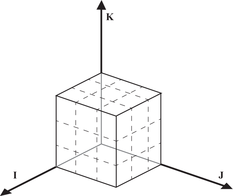
Figure 1. An example of a $3\times 3\times 3$ table.

Algorithm 3.6 (Store structures in the zero-one table).

This algorithm stores the structures, including zeros and ones, in the observed table $\mathchoice{\mbox{\boldmath$\displaystyle\bf x$}}{\mbox{\boldmath$\textstyle\bf x$}}{\mbox{\boldmath$\scriptstyle\bf x$}}{\mbox{\boldmath$\scriptscriptstyle\bf x$}}_{0}$. The output will be used to avoid trivial cases in sampling. The output $A$ and $B$ matrices both have the same dimension with $\mathchoice{\mbox{\boldmath$\displaystyle\bf x$}}{\mbox{\boldmath$\textstyle\bf x$}}{\mbox{\boldmath$\scriptstyle\bf x$}}{\mbox{\boldmath$\scriptscriptstyle\bf x$}}_{0}$, so the cell value in $A$ will be $1$ if the position is structured and $0$ if not. The matrix $B$ is only for structure $1$’s. We consider sampling a table without structure $1$’s, that is, a table with new marginals: $X^{*}_{ij+}=X_{ij+}-\sum_{k=1}^{l}B_{ijk}=X_{ij+}-B_{ij+}$, $X^{*}_{i+k}=X_{i+k}-\sum_{j=1}^{n}B_{ijk}=X_{i+k}-B_{i+k}$, and $X^{*}_{+jk}=X_{+jk}-\sum_{i=1}^{m}B_{ijk}=X_{+jk}-B_{+jk}$ for $i=1,2,\ldots,m\mbox{, }j=1,2,\ldots,n$, and $k=1,2,\ldots,l$.

• The observed marginals $X_{ij+}$, $X_{i+k}$, and $X_{+jk}$ for $i=1,2,\ldots,m\mbox{, }j=1,2,\ldots,n$, and $k=1,2,\ldots,l$.

• Matrix $A$ and $B$, new marginals $X^{*}_{ij+}$, $X^{*}_{i+k}$, and $X^{*}_{+jk}$ for $i=1,2,\ldots,m\mbox{, }j=1,2,\ldots,n$, and $k=1,2,\ldots,l$.

• 1. Check all marginals in direction I. For $i=1,2,\ldots,m$:
     If $X_{+jk}=0$, $A_{i^{\prime}jk}=1$, for all $i^{\prime}=1,2,\ldots,m$ and $A_{i^{\prime}jk}=0$;
     If $X_{+jk}=1$, $A_{i^{\prime}jk}=1$ and $B_{i^{\prime}jk}=1$, for all $i^{\prime}=1,2,\ldots,m$ and $A_{i^{\prime}jk}=0$.
     

  2. Check all marginals in direction J. For $j=1,2,\ldots,n$:
     If $X_{i+k}=0$, $A_{ij^{\prime}k}=1$, for all $j^{\prime}=1,2,\ldots,n$ and $A_{ij^{\prime}k}=0$;
     If $X_{i+k}=1$, $A_{ij^{\prime}k}=1$ and $B_{ij^{\prime}k}=1$, for all $j^{\prime}=1,2,\ldots,n$ and $A_{ij^{\prime}k}=0$.
     

  3. Check all marginals in direction K. For $k=1,2,\ldots,l$:
     If $X_{ij+}=0$, $A_{ijk^{\prime}}=1$, for all $k^{\prime}=1,2,\ldots,l$ and $A_{ijk^{\prime}}=0$;
     If $X_{ij+}=1$, $A_{ijk^{\prime}}=1$ and $B_{ijk^{\prime}}=1$, for all $k^{\prime}=1,2,\ldots,l$ and $A_{ijk^{\prime}}=0$.
     

  4. If any changes made in step (1), (2) or (3), come back to (1), else stop.

  5. Compute new marginals:
     $X^{*}_{ij+}=X_{ij+}-B_{ij+}$, $X^{*}_{i+k}=X_{i+k}-B_{i+k}$, and $X^{*}_{+jk}=X_{+jk}-B_{+jk}$ for $i=1,2,\ldots,m\mbox{, }j=1,2,\ldots,n$, and $k=1,2,\ldots,l$.

Algorithm 3.7 (Generate a two-way table with given marginals).

This algorithm is used to generate a layer (fixed $i$) of the three-way table, with the probability of the sampled layer.

• Row sums $r^{*}_{j}$ and column sums $c^{*}_{k}$, $j=1,2,\ldots,n$, and $k=1,2,\ldots,l$; structures $A$; marginals on direction I: $X_{+jk}$ for $i=1,2,\ldots,m$.

• A sampled table and its probability. Return $0$ if the process fails.

• 1. Order all columns with decreasing sums.

  2. Generate the column (along the direction $K$) with the largest sum, the weights used in CP are shown in equation (3.5). Notice that $k$ relates to each specific cell in the column, $r_{k}$ and $c_{k}$ which are the row sums in the direction $J$ and $I$, respectively. $g^{r_{0}}_{k}$ and $g^{c_{0}}_{k}$ are the number of structures in the rows of the direction $J$ and $I$, respectively. The probability of the generated column will be returned if the process succeeds, while $0$ may be returned in this step if it does not exist.

  3. Delete the generated column in (2), and for the remaining subtable, do the following:

     1. If only one column is left, fill it with fixed marginals and go to (4).

     2. If (a) is not true, check all marginals to see if there are any new structures caused by step (2). We need to avoid trivial cases by doing this. Go back to (1) with new marginals and structures.

  4. Return generated matrix as the new layer and its CP probability. If failed, return $0$.

Algorithm 3.8 (SIS with CP for sampling a three-way zero-one table).

We describe an algorithm to sample a three-way zero-one table $\textstyle\bf X$ with given marginals $X_{ij+}$, $X_{i+k}$, and $X_{+jk}$ for $i=1,2,\ldots,m\mbox{, }j=1,2,\ldots,n$, and $k=1,2,\ldots,l$ via the SIS with CP.

• The observed table $\mathchoice{\mbox{\boldmath$\displaystyle\bf x$}}{\mbox{\boldmath$\textstyle\bf x$}}{\mbox{\boldmath$\scriptstyle\bf x$}}{\mbox{\boldmath$\scriptscriptstyle\bf x$}}_{0}$.

• The sampled table $\textstyle\bf x$.

• 1. Compute the marginals $X_{ij+}$, $X_{i+k}$, and $X_{+jk}$ for $i=1,2,\ldots,m\mbox{, }j=1,2,\ldots,n$, and $k=1,2,\ldots,l$.

  2. Use Algorithm 3.6 to compute the structure tables $A$ and $B$. Consider the new marginals in the output as the sampling marginals.

  3. For the sampling marginals, do the SIS:

     1. Delete the layers filled by structures; consider the left-over subtable.

     2. Consider the layers in direction $I$ ($i$ varies). Sum within all layers and order them from the largest to smallest.

     3. Consider the layer with the largest sum and plug in the structure table $A$ from Algorithm 3.7 to generate a sample for this layer. The algorithm may return $0$ if the sampling fails.

     4. Delete the generated layer in (c), and for the remaining subtable, do the following:

        1. If only one layer left, fill it with fixed marginals and go to (e).

        2. else, go back to (2) with new marginals.

     5. Add the sampled table with table $B$ (the structure $1$’s table).

  4. Return the table in (e) and the same probability with the sampled table. Return $0$ if failed.

4. Four or higher dimensional zero-one tables

In this section we consider a $d$-way zero-one table under the no $d$-way interaction model for $d\in{\mathbb{N}}$ and $d>3$. Let $\mathchoice{\mbox{\boldmath$\displaystyle\bf X$}}{\mbox{\boldmath$\textstyle\bf X$}}{\mbox{\boldmath$\scriptstyle\bf X$}}{\mbox{\boldmath$\scriptscriptstyle\bf X$}}=(X_{i_{1}\ldots i_{d}})$ be a zero-one contingency table of size $(n_{1}\times\cdots\times n_{d})$, where $n_{i}\in{\mathbb{N}}$ for $i=1,\ldots,d$. The sufficient statistics under the no $d$-way interaction model are

(4.1) $$\begin{array}[]{l}X_{+i_{2}\ldots i_{d}},\,X_{i_{1}+i_{3}\ldots i_{d}},\,\ldots,X_{i_{1}\ldots i_{d-1}+},\\ \text{for }i_{1}=1,\ldots,n_{1},\,i_{2}=1,\ldots,n_{2},\ldots,i_{d}=1,\ldots,n_{d}.\\ \end{array}$$

For each $i_{1}^{0}\in\{1,\ldots,n_{1}\},\ldots,i_{d-1}^{0}\in\{1,\ldots,n_{d}\}$, we say the column of the entries for a marginal $X_{i_{1}\ldots i_{j-1}+i_{j+1}\ldots i_{d}}$ the $(i_{0},\ldots,i_{j-1},i_{j+1},\ldots,i_{d})$th column of $\textstyle\bf X$. For each $i_{1}^{0}\in\{1,\ldots,n_{1}\},\ldots,i_{d-1}^{0}\in\{1,\ldots,n_{d-1}\}$, we consider the $(i_{1}^{0},\ldots,i_{d-1}^{0})$th column for the $d$th factor. Let $l_{0}=X_{i_{1}^{0},\ldots,i_{d-1}^{0}+}$. Let $r_{k}^{j}=X_{i_{1}^{0}\ldots i_{j-1}^{0}+i_{j+1}^{0}\ldots i_{d-1}^{0}k}$ for fixed $k\in\{1,\ldots,n_{d}\}$. For sampling a zero-one $d$-way table $\textstyle\bf X$, we set

(4.2) $$p_{k}:=\frac{\prod_{j=1}^{d-1}r_{k}^{j}}{\prod_{j=1}^{d-1}r_{k}^{j}+\prod_{j=1}^{d-1}(n_{j}-r_{k}^{j})}.$$

Remark 4.1.

We assume that we do not have trivial cases, namely, $1\leq r_{k}^{j}\leq n_{j}-1$ for $j=1,\ldots,d$.

Theorem 4.2.

For the uniform distribution over all $d$-way zero-one contingency tables $\mathchoice{\mbox{\boldmath$\displaystyle\bf X$}}{\mbox{\boldmath$\textstyle\bf X$}}{\mbox{\boldmath$\scriptstyle\bf X$}}{\mbox{\boldmath$\scriptscriptstyle\bf X$}}=(X_{i_{1}\ldots i_{d}})$ of size $(n_{1}\times\cdots\times n_{d})$, where $n_{i}\in{\mathbb{N}}$ for $i=1,\ldots,d$ with marginals $l_{0}=X_{i_{1}^{0},\ldots,i_{d-1}^{0}+}$, and $r_{k}^{j}=X_{i_{1}^{0}\ldots i_{j-1}^{0}+i_{j+1}^{0}\ldots i_{d-1}^{0}k}$ for $k\in\{1,\ldots,n_{d}\}$, the marginal distribution of the fixed marginal $l_{0}$ is the same as the conditional distribution of $Z$ defined by (3.1) given $S_{Z}=l_{0}$ with

$$p_{k}:=\frac{\prod_{j=1}^{d-1}r_{k}^{j}}{\prod_{j=1}^{d-1}r_{k}^{j}+\prod_{j=1}^{d-1}(n_{j}-r_{k}^{j})}.$$

Proof.

The proof is similar to the proof for Theorem 3.2, we just extend the same argument to a $d$-way zero-one table under the no $d$-way interaction model with the probability

$$p_{k}=\frac{\prod_{j=1}^{d-1}{n_{j}-1\choose r_{k}^{j}-1}}{\prod_{j=1}^{d-1}{n_{j}-1\choose r_{k}^{j}-1}+\prod_{j=1}^{d-1}{n_{j}-1\choose r_{k}^{j}}}=\frac{\prod_{j=1}^{d-1}r_{k}^{j}}{\prod_{j=1}^{d-1}r_{k}^{j}+\prod_{j=1}^{d-1}(n_{j}-r_{k}^{j})}.$$

∎

During the intermediary steps of our SIS procedure via CP on a three-way zero-one table there will be some columns for the $d$th factor with trivial cases. In that case we have to treat them as structural zeros in the $k$th slice for some $k\in\{1,\ldots,l\}$. In that case we have to use the probabilities for the distribution in (3.1) as follows:

(4.3) $$p_{k}:=\frac{\prod_{j=1}^{d-1}r_{k}^{j}}{\prod_{j=1}^{d-1}r_{k}^{j}+\prod_{j=1}^{d-1}(n_{j}-r_{k}^{j}-g_{k}^{j})}.$$

where $g_{k}^{j}$ is the number of structural zeros in the $(i_{1}^{0},\ldots,i_{j-1}^{0},i_{j+1}^{0},\ldots,i_{d-1}^{0}k)$th column of $\textstyle\bf X$. Thus we have weights:

(4.4) $$w_{k}=\frac{\prod_{j=1}^{d-1}r_{k}^{j}}{\prod_{j=1}^{d-1}(n_{j}-r_{k}^{j}-g_{k}^{j})}.$$

Theorem 4.3.

For the uniform distribution over all $d$-way zero-one contingency tables $\mathchoice{\mbox{\boldmath$\displaystyle\bf X$}}{\mbox{\boldmath$\textstyle\bf X$}}{\mbox{\boldmath$\scriptstyle\bf X$}}{\mbox{\boldmath$\scriptscriptstyle\bf X$}}=(X_{i_{1}\ldots i_{d}})$ of size $(n_{1}\times\cdots\times n_{d})$, where $n_{i}\in{\mathbb{N}}$ for $i=1,\ldots,d$ with marginals $l_{0}=X_{i_{1}^{0},\ldots,i_{d-1}^{0}+}$, and $r_{k}^{j}=X_{i_{1}^{0}\ldots i_{j-1}^{0}+i_{j+1}^{0}\ldots i_{d-1}^{0}k}$ for $k\in\{1,\ldots,n_{d}\}$, the marginal distribution of the fixed marginal $l_{0}$ is the same as the conditional distribution of $Z$ defined by (3.1) given $S_{Z}=l_{0}$ with

$$p_{k}:=\frac{\prod_{j=1}^{d-1}r_{k}^{j}}{\prod_{j=1}^{d-1}r_{k}^{j}+\prod_{j=1}^{d-1}(n_{j}-r_{k}^{j}-g_{k}^{j})}$$

where $g_{k}^{j}$ is the number of structural zeros in the $(i_{1}^{0},\ldots,i_{j-1}^{0},i_{j+1}^{0},\ldots,i_{d-1}^{0}k)$th column of $\textstyle\bf X$.

Proof.

The proof is similar to the proof for Theorem 3.4, we just extend the same argument to a $d$-way zero-one table under the no $d$-way interaction model with the probability

$$p_{k}=\frac{\prod_{j=1}^{d-1}{n_{j}-1-g^{j}_{k}\choose r_{k}^{j}-1}}{\prod_{j=1}^{d-1}{n_{j}-1-g^{j}_{k}\choose r_{k}^{j}-1}+\prod_{j=1}^{d-1}{n_{j}-1-g^{j}_{k}\choose r_{k}^{j}}}=\frac{\prod_{j=1}^{d-1}r_{k}^{j}}{\prod_{j=1}^{d-1}r_{k}^{j}+\prod_{j=1}^{d-1}(n_{j}-r_{k}^{j}-g^{j}_{k})}.$$

∎

5. Computational examples

For our simulation study we used the software package R [10]. We count the exact numbers of tables via the software LattE [5] for small examples in this section (Examples (5.2) to (5.13)).

When the contingency tables are large and/or the models are complicated, it is very difficult to obtain the exact number of tables. Thus we need a good measurement of accuracy in the estimated number of tables. In [3], they used the coefficient of variation ($cv^{2}$):

$$cv^{2}=\frac{var_{q}\{p({\bf X})/q({\bf X})\}}{{\mathbb{E}}^{2}_{q}\{p({\bf X})/q({\bf X})\}}$$

which is equal to $var_{q}\{1/q({\bf X})\}/{\mathbb{E}}^{2}_{q}\{1/q({\bf X})\}$ for the problem of estimating the number of tables. The value of $cv^{2}$ is simply the chi-square distance between the two distributions $p^{\prime}$ and $q$, which means the smaller it is, the closer the two distributions are. In [3] they estimated $cv^{2}$ by:

$$cv^{2}\approx\frac{\sum_{i=1}^{N}\{1/q({\bf X_{i}})-\left[\sum_{j=1}^{N}1/q({\bf X_{j}})\right]/N\}^{2}/(N-1)}{\left\{\left[\sum_{j=1}^{N}1/q({\bf X_{j}})\right]/N\right\}^{2}},$$

where ${\bf X_{1}},\ldots,{\bf X_{N}}$ are tables drawn iid from $q({\bf X})$. When we have rejections, we compute the variance using only accepted tables. In this paper we also investigated relations with the exact numbers of tables and $cv^{2}$ when we have rejections.

In this section, we define the three two-way marginal matrices as following:
Suppose we have an observed table $\mathchoice{\mbox{\boldmath$\displaystyle\bf x$}}{\mbox{\boldmath$\textstyle\bf x$}}{\mbox{\boldmath$\scriptstyle\bf x$}}{\mbox{\boldmath$\scriptscriptstyle\bf x$}}=(x_{ijk})_{m\times n\times l}$, $i=1,2,\ldots,m\mbox{, }j=1,2,\ldots,n$, and $k=1,2,\ldots,l$;
Define: $si=(X_{+jk})_{n\times l}$, $sj=(X_{i+k})_{m\times l}$, and $sk=(X_{ij+})_{m\times n}$.

Example 5.1 (The 3-dimension Semimagic Cube).

Suppose $si$, $sj$, and $sk$ are all $3\times 3$ matrices with all 1’s inside, that is:

$$si=sj=sk=\begin{array}[]{|c|c|c|}\hline\cr 1&1&1\\ \hline\cr 1&1&1\\ \hline\cr 1&1&1\\ \hline\cr\end{array}$$

The real number of tables is $12$. We took $114.7$ seconds to run $10,000$ samples in the SIS, the estimator is $12$, acceptance rate is $100$%. Actually, we found that if the acceptance rate is $100$%, then sample size does not matter in the estimation.

We used R to produce more examples. Examples (5.2) to (5.13) are constructed by the same code but with different values for parameters. We used the R package “Rlab” for the following code.

    seed=6; m=3; n=3; l=4; prob=0.8; N=1000; k=200
    set.seed(seed)
    A=array(rbern(m*n*l,prob),c(m,n,l))
    outinfo=tabinfo(A)
    numtable(N,outinfo,k)

Here prob is the probability of getting $1$ for every Bernoulli variable, and $N$ is the sample size (the total number of tables sampled, including both acceptances and rejections). Notice that $cv^{2}$ is defined as $\frac{Var}{Mean^{2}}$.

Example 5.2 (seed=6; m=3; n=3; l=4; prob=0.8).

Suppose $si$, $sj$, and $sk$ are as following, respectively:

$$\begin{array}[]{|c|c|c|c|}\hline\cr 2&2&2&2\\ \hline\cr 1&3&2&2\\ \hline\cr 2&3&3&2\\ \hline\cr\end{array}\,,\ \ \ \begin{array}[]{|c|c|c|c|}\hline\cr 2&3&2&2\\ \hline\cr 1&3&3&3\\ \hline\cr 2&2&2&1\\ \hline\cr\end{array}\,,\ \ \ \begin{array}[]{|c|c|c|}\hline\cr 3&3&3\\ \hline\cr 3&3&4\\ \hline\cr 2&2&3\\ \hline\cr\end{array}\,.$$

The real number of tables is $3$. An estimator is $3.00762$ with $cv^{2}=0.0708$. The whole process took $13.216$ seconds (in R) with a $100$% acceptance rate.

Example 5.3 (seed=60; m=3; n=4; l=4; prob=0.5).

Suppose $si$, $sj$, and $sk$ are as following, respectively:

$$\begin{array}[]{|c|c|c|c|}\hline\cr 2&2&2&1\\ \hline\cr 1&1&1&0\\ \hline\cr 1&1&1&2\\ \hline\cr 1&1&2&3\\ \hline\cr\end{array}\,,\ \ \ \begin{array}[]{|c|c|c|c|}\hline\cr 3&3&2&1\\ \hline\cr 1&0&2&2\\ \hline\cr 1&2&2&3\\ \hline\cr\end{array}\,,\ \ \ \begin{array}[]{|c|c|c|c|}\hline\cr 3&2&2&2\\ \hline\cr 1&0&2&2\\ \hline\cr 3&1&1&3\\ \hline\cr\end{array}\,.$$

The real number of tables is $5$. An estimator is $4.991026$ with $cv^{2}=0.1335$. The whole process took $17.016$ seconds (in R) with a $100$% acceptance rate.

Example 5.4 (seed=61; m=3; n=4; l=4; prob=0.5).

Suppose $si$, $sj$, and $sk$ are as following, respectively:

$$\begin{array}[]{|c|c|c|c|}\hline\cr 1&2&2&1\\ \hline\cr 0&1&1&2\\ \hline\cr 1&0&2&1\\ \hline\cr 0&1&3&2\\ \hline\cr\end{array}\,,\ \ \ \begin{array}[]{|c|c|c|c|}\hline\cr 1&2&3&2\\ \hline\cr 1&1&2&3\\ \hline\cr 0&1&3&1\\ \hline\cr\end{array}\,,\ \ \ \begin{array}[]{|c|c|c|c|}\hline\cr 3&1&1&3\\ \hline\cr 1&2&2&2\\ \hline\cr 2&1&1&1\\ \hline\cr\end{array}\,.$$

The real number of tables is $8$. An estimator is 8.04964 with $cv^{2}=0.2389$. The whole process took $16.446$ seconds (in R) with a $100$% acceptance rate.

Example 5.5 (seed=240; m=4; n=4; l=4; prob=0.5).

Suppose $si$, $sj$, and $sk$ are as following, respectively:

$$\begin{array}[]{|c|c|c|c|}\hline\cr 2&3&3&2\\ \hline\cr 1&3&2&1\\ \hline\cr 1&2&3&0\\ \hline\cr 4&2&2&2\\ \hline\cr\end{array}\,,\ \ \ \begin{array}[]{|c|c|c|c|}\hline\cr 2&2&4&1\\ \hline\cr 3&2&2&2\\ \hline\cr 2&3&3&1\\ \hline\cr 1&3&1&1\\ \hline\cr\end{array}\,,\ \ \ \begin{array}[]{|c|c|c|c|}\hline\cr 2&2&3&2\\ \hline\cr 3&2&1&3\\ \hline\cr 3&2&2&2\\ \hline\cr 2&1&0&3\\ \hline\cr\end{array}\,.$$

The real number of tables is $8$. An estimator is 8.039938 with $cv^{2}=0.2857$. The whole process took $23.612$ seconds (in R) with a $100$% acceptance rate.

Example 5.6 (seed=1240; m=4; n=4; l=4; prob=0.5).

Suppose $si$, $sj$, and $sk$ are as following, respectively:

$$\begin{array}[]{|c|c|c|c|}\hline\cr 2&3&2&3\\ \hline\cr 1&2&3&2\\ \hline\cr 2&2&3&2\\ \hline\cr 3&2&3&2\\ \hline\cr\end{array}\,,\ \ \ \begin{array}[]{|c|c|c|c|}\hline\cr 1&4&1&3\\ \hline\cr 4&2&4&2\\ \hline\cr 1&2&4&3\\ \hline\cr 2&1&2&1\\ \hline\cr\end{array}\,,\ \ \ \begin{array}[]{|c|c|c|c|}\hline\cr 2&2&2&3\\ \hline\cr 3&3&3&3\\ \hline\cr 3&2&2&3\\ \hline\cr 2&1&2&1\\ \hline\cr\end{array}\,.$$

The real number of tables is $28$. An estimator is $26.89940$ with $cv^{2}=1.0306$. The whole process took $29.067$ seconds (in R) with a $100$% acceptance rate. It converges even better for sample size 5000: the estimator becomes $28.0917$, with $cv^{2}=1.2070$.

Example 5.7 (seed=2240; m=4; n=4; l=4; prob=0.5).

Suppose $si$, $sj$, and $sk$ are as following, respectively:

$$\begin{array}[]{|c|c|c|c|}\hline\cr 1&2&3&1\\ \hline\cr 2&3&2&3\\ \hline\cr 2&4&2&1\\ \hline\cr 2&1&4&1\\ \hline\cr\end{array}\,,\ \ \ \begin{array}[]{|c|c|c|c|}\hline\cr 2&3&2&0\\ \hline\cr 3&2&3&2\\ \hline\cr 1&3&3&1\\ \hline\cr 1&2&3&3\\ \hline\cr\end{array}\,,\ \ \ \begin{array}[]{|c|c|c|c|}\hline\cr 2&1&2&2\\ \hline\cr 3&2&3&2\\ \hline\cr 1&4&2&1\\ \hline\cr 1&3&2&3\\ \hline\cr\end{array}\,.$$

The real number of tables is $4$. An estimator is $3.98125$ with $cv^{2}=0.0960$. The whole process took $26.96$ seconds (in R) with a $100$% acceptance rate.

Example 5.8 (seed=3340; m=4; n=4; l=4; prob=0.5).

Suppose $si$, $sj$, and $sk$ are as following, respectively:

$$\begin{array}[]{|c|c|c|c|}\hline\cr 2&4&1&3\\ \hline\cr 1&2&1&2\\ \hline\cr 1&1&0&3\\ \hline\cr 4&1&0&2\\ \hline\cr\end{array}\,,\ \ \ \begin{array}[]{|c|c|c|c|}\hline\cr 2&1&1&2\\ \hline\cr 3&1&1&3\\ \hline\cr 1&2&0&2\\ \hline\cr 2&4&0&3\\ \hline\cr\end{array}\,,\ \ \ \begin{array}[]{|c|c|c|c|}\hline\cr 3&1&1&1\\ \hline\cr 3&1&2&2\\ \hline\cr 1&2&1&1\\ \hline\cr 3&2&1&3\\ \hline\cr\end{array}\,.$$

The real number of tables is $2$. An estimator is $2$ with $cv^{2}=0$. The whole process took $15.214$ seconds (in R) with a $100\%$ acceptance rate.

Example 5.9 (seed=3440; m=4; n=4; l=4; prob=0.5).

Suppose $si$, $sj$, and $sk$ are as following, respectively:

$$\begin{array}[]{|c|c|c|c|}\hline\cr 1&3&1&3\\ \hline\cr 1&1&2&2\\ \hline\cr 2&3&1&0\\ \hline\cr 3&2&2&3\\ \hline\cr\end{array}\,,\ \ \ \begin{array}[]{|c|c|c|c|}\hline\cr 2&2&2&2\\ \hline\cr 2&1&2&1\\ \hline\cr 1&3&1&2\\ \hline\cr 2&3&1&3\\ \hline\cr\end{array}\,,\ \ \ \begin{array}[]{|c|c|c|c|}\hline\cr 3&1&1&3\\ \hline\cr 1&2&1&2\\ \hline\cr 2&0&3&2\\ \hline\cr 2&3&1&3\\ \hline\cr\end{array}\,.$$

The real number of tables is $12$. An estimator is $12.04838$ with $cv^{2}=0.7819733$. The whole process took $27.074$ seconds (in R) with a $85.9$% acceptance rate.

Example 5.10 (seed=5440; m=4; n=4; l=4; prob=0.5).

Suppose $si$, $sj$, and $sk$ are as following, respectively:

$$\begin{array}[]{|c|c|c|c|}\hline\cr 2&1&0&1\\ \hline\cr 2&3&1&2\\ \hline\cr 3&1&2&1\\ \hline\cr 1&3&2&2\\ \hline\cr\end{array}\,,\ \ \ \begin{array}[]{|c|c|c|c|}\hline\cr 2&3&2&1\\ \hline\cr 2&1&2&3\\ \hline\cr 2&1&0&1\\ \hline\cr 2&3&1&1\\ \hline\cr\end{array}\,,\ \ \ \begin{array}[]{|c|c|c|c|}\hline\cr 1&2&2&3\\ \hline\cr 1&1&3&3\\ \hline\cr 1&3&0&0\\ \hline\cr 1&2&2&2\\ \hline\cr\end{array}\,.$$

The real number of tables is $9$. An estimator is $8.882672$ with $cv^{2}=0.7701368$. The whole process took $30.171$ seconds (in R) with a $100$% acceptance rate. Another result for the same sample size is: an estimator is $8.521734$, $cv^{2}=0.6695902$. You can find that the latter has a slightly better $cv^{2}$ but a slightly worse estimator. We’ll discuss more in Section 7.

Example 5.11 (seed=122; m=4; n=4; l=5; prob=0.2).

Suppose $si$, $sj$, and $sk$ are as following, respectively:

$$\begin{array}[]{|c|c|c|c|c|}\hline\cr 2&0&3&3&2\\ \hline\cr 0&0&1&0&0\\ \hline\cr 1&0&1&1&1\\ \hline\cr 0&1&0&1&0\\ \hline\cr\end{array}\,,\ \ \ \begin{array}[]{|c|c|c|c|c|}\hline\cr 1&0&0&2&1\\ \hline\cr 1&0&2&1&1\\ \hline\cr 1&1&1&1&1\\ \hline\cr 0&0&2&1&0\\ \hline\cr\end{array}\,,\ \ \ \begin{array}[]{|c|c|c|c|}\hline\cr 3&0&0&1\\ \hline\cr 4&1&0&0\\ \hline\cr 1&0&3&1\\ \hline\cr 2&0&1&0\\ \hline\cr\end{array}\,.$$

The real number of tables is $5$. An estimator is $4.93625$ with $cv^{2}=0.2035$. The whole process took $21.325$ seconds (in R) with a $100$% acceptance rate.

Example 5.12 (seed=222; m=4; n=4; l=5; prob=0.2).

Suppose $si$, $sj$, and $sk$ are as following, respectively:

$$\begin{array}[]{|c|c|c|c|c|}\hline\cr 1&0&1&1&1\\ \hline\cr 2&1&0&1&2\\ \hline\cr 0&1&1&1&0\\ \hline\cr 1&1&1&1&1\\ \hline\cr\end{array}\,,\ \ \ \begin{array}[]{|c|c|c|c|c|}\hline\cr 2&1&0&0&2\\ \hline\cr 1&2&1&2&1\\ \hline\cr 1&0&1&1&1\\ \hline\cr 0&0&1&1&0\\ \hline\cr\end{array}\,,\ \ \ \begin{array}[]{|c|c|c|c|}\hline\cr 2&3&0&0\\ \hline\cr 1&3&2&1\\ \hline\cr 0&0&1&3\\ \hline\cr 1&0&0&1\\ \hline\cr\end{array}\,.$$

The real number of tables is $2$. An estimator is $2$ with $cv^{2}=0$. The whole process took $19.064$ seconds (in R) with a $100$% acceptance rate.

Example 5.13 (seed=322; m=4; n=4; l=5; prob=0.2).

Suppose $si$, $sj$, and $sk$ are as following, respectively:

$$\begin{array}[]{|c|c|c|c|c|}\hline\cr 1&1&1&1&1\\ \hline\cr 1&1&1&1&1\\ \hline\cr 1&2&0&0&1\\ \hline\cr 2&0&1&1&2\\ \hline\cr\end{array}\,,\ \ \ \begin{array}[]{|c|c|c|c|c|}\hline\cr 0&0&1&1&0\\ \hline\cr 1&0&1&0&1\\ \hline\cr 2&2&0&1&2\\ \hline\cr 2&2&1&1&2\\ \hline\cr\end{array}\,,\ \ \ \begin{array}[]{|c|c|c|c|}\hline\cr 0&2&0&0\\ \hline\cr 1&0&0&2\\ \hline\cr 1&3&1&2\\ \hline\cr 3&0&3&2\\ \hline\cr\end{array}\,.$$

The real number of tables is $5$. An estimator is $4.992$ with $cv^{2}=0.2179682$. The whole process took $23.25$ seconds (in R) with a $85.2$% acceptance rate.

Summary 5.14 (Summarize the results from Example (5.2) to Example (5.13)).

This is only a summary of main results of those examples in Table 1. For all results here, we set the sample size $1,000$. We will discuss these results in Section 7.

Dimension	Example	# tables	Estimation	$cv^{2}$	Acceptance rate
$3\times 3\times 4$	5.2	3	3.00762	0.0708	100%
$3\times 4\times 4$	5.3	5	4.991026	0.1335	100%
	5.4	8	8.04964	0.2389	100%
$4\times 4\times 4$	5.5	8	8.039938	0.2857	100%
	5.6	28	26.89940	1.0306	100%
	5.7	4	3.98125	0.0960	100%
	5.8	2	2	0	100%
	5.9	12	12.04838	0.7820	85.9%
	5.10	9	8.882672	0.7701	100%
$4\times 4\times 5$	5.11	5	4.93625	0.2035	100%
	5.12	2	2	0	100%
	5.13	5	4.992	0.2180	85.2%

Table 1. Summary of Examples (5.2) - (5.13)

Example 5.15 (High-dimension Semimagic Cubes).

In this example, we consider $m\times n\times l$ tables for $m=n=l=4,\ldots,10$ such that each marginal sum equals to $1$. The results are summarized in Table 2.

Dimension $m$	$N$	CPU time (sec)	Estimation	$cv^{2}$	Acceptance rate
$4$	$1000$	$32.44$	568.944	0.26	$100\%$
	$10000$	$324.18$	571.1472	0.27	$100\%$
$5$	$1000$	$60.39$	161603.5	0.18	$99\%$
	$10000$	$605.45$	161439.3	0.18	$99.2\%$
$6$	$1000$	$102.66$	801634023	0.58	$98.3\%$
	$10000$	$1038.46$	819177227	0.45	$98.8\%$
$7$	$1000$	$158.55$	6.08928e+13	0.60	$97\%$
	$10000$	$1590.84$	6.146227e+13	0.64	$97.7\%$
$8$	$1000$	$234.53$	1.080208e+20	1.07	$95.6\%$
	$10000$	$2300.91$	1.099627e+20	1.00	$96.5\%$
$9$	$1000$	$329.17$	5.845308e+27	1.46	$94\%$
	$10000$	$3238.1$	5.684428e+27	1.59	$95.3\%$
$10$	$1000$	$451.24$	9.648942e+36	1.44	$93.3\%$
	$10000$	$4425.12$	9.73486e+36	1.73	$93.3\%$

Table 2. Summary of computational results on $m\times n\times l$ tables for $m=n=l=4,\ldots,10$. The all marginal sums are equal to one in this example.

Example 5.16 (High-dimension Semimagic Cubes continues).

In this example, we consider $m\times n\times l$ tables for $m=n=l=4,\ldots,10$ such that each marginal sum equals to $s$. The results are summarized in Table 3. In this example, we set the sample size $N=1000$.

Dimension $m$	$s$	CPU time (sec)	Estimation	$cv^{2}$	Acceptance rate
$4$	$2$	$27.1$	51810.36	0.66	$97.7\%$
$5$	$2$	$58.1$	25196288574	1.69	$97.5\%$
$6$	$2$	$97.1$	6.339628e+18	2.56	$94.8\%$
	$3$	$99.3$	1.269398e+22	2.83	$96.5\%$
$7$	$2$	$150.85$	1.437412e+30	4.76	$93.1\%$
	$3$	$166.68$	2.365389e+38	25.33	$96.7\%$
$8$	$2$	$229.85$	5.369437e+44	6.68	$89.8\%$
	$3$	$256.70$	3.236556e+59	7.05	$94.5\%$
	$4$	$328.52$	2.448923e+64	11.98	$94.3\%$
$9$	$2$	$319.32$	4.416787e+62	8.93	$85.7\%$
	$3$	$376.67$	7.871387e+85	15.23	$91.6\%$
	$4$	$549.73$	2.422237e+97	14.00	$93.4\%$
$10$	$2$	$429.19$	2.166449e+84	10.46	$83.3\%$
	$3$	$527.14$	6.861123e+117	26.62	$90\%$
	$4$	$883.34$	3.652694e+137	33.33	$93.8\%$
	$5$	$1439.50$	1.315069e+144	46.2	$91.3\%$

Table 3. Summary of computational results on $m\times n\times l$ tables for $m=n=l=4,\ldots,10$. The all marginal sums are equal to $s$ in this example. The sample $N=1000$ in this example.

Example 5.17 (Bootstrap-t confidence interval of Semimagic Cubes).

As we can see that in Table 3, generally we have larger $cv^{2}$ when the number of tables is larger, and in this case, the estimator we get via the SIS procedure might vary greatly in different iterations. Therefore, we might want to compute a $(1-\alpha)100\%$ confidence interval for each estimator via a non-parametric bootstrap method (see Appendix A for a pseudo code for a non-parametric bootstrap method to get the $(1-\alpha)100\%$ confidence interval for $|\Sigma|$). See Table 4 for some results of Bootstrap-t $95\%$ confidence intervals ($\alpha=0.05$).

		Estimation			$cv^{2}$
Dim	s	$\widehat{|\Sigma|}$	Lower $95\%$	Upper $95\%$	$\widehat{cv^{2}}$	Lower $95\%$	Upper $95\%$	Acceptance Rate
7	2	1.306480e+30	1.156686e+30	1.468754e+30	3.442306	2.678507	4.199513	$93.3\%$
	3	3.033551e+38	2.245910e+38	4.087225e+38	22.84399	8.651207	35.080408	$96.2\%$
8	2	5.010225e+44	4.200752e+44	5.902405e+44	6.712335	4.539368	8.590578	$90.4\%$
	3	2.902294e+59	2.389625e+59	3.484405e+59	9.047914	5.680128	12.797488	$93.1\%$
	4	2.474874e+64	1.847911e+64	3.295986e+64	21.53559	5.384647	32.166086	$94.6\%$
9	2	4.548401e+62	3.682882e+62	5.593370e+62	10.07973	4.886817	15.406899	$87.1\%$
	3	9.702672e+85	7.189849e+85	1.250875e+86	18.65302	11.33462	23.77980	$92.5\%$
	4	2.023034e+97	1.547951e+97	2.561084e+97	14.96126	10.20331	19.09515	$92.2\%$
10	2	2.570344e+84	1.908609e+84	3.339243e+84	17.83684	9.785778	24.231544	$84.8\%$
	3	8.68783e+117	5.92233e+117	1.22271e+118	29.67200	18.64549	37.64892	$90.2\%$
	4	4.12634e+137	2.94789e+137	5.52727e+137	23.36831	15.32719	31.02614	$92\%$
	5	1.54956e+144	9.85557e+143	2.24043e+144	39.06521	20.23674	53.60838	$91.8\%$

Table 4. Summary of confidence intervals. Dimensions and marginals$=s$ are defined same with Table 3. $\widehat{|\Sigma|}$ means an estimator of ${|\Sigma|}$ and $\widehat{cv^{2}}$ is an estimator of $cv^{2}$. The sample size for the SIS procedure is $N=1000$ and the sample size for bootstraping is $B=5000$. Only cases with relatively large $cv^{2}$ are involved.

6. Experiment with Sampson’s data set

Sampson recorded the social interactions among a group of monks when he was visiting there as an experimenter on vision. He collected numerous sociometric rankings [1, 8]. The data is organized as a $18\times 18\times 10$ table and one can find the full data sets at http://vlado.fmf.uni-lj.si/pub/networks/data/ucinet/UciData.htm#sampson. Each layer of $18\times 18$ table represents a social relation between 18 monks at some time point. Most of the present data are retrospective, collected after the breakup occurred. They concern a period during which a new cohort entered the monastery near the end of the study but before the major conflict began. The exceptions are “liking” data gathered at three times: SAMPLK1 to SAMPLK3 - that reflect changes in group sentiment over time (SAMPLK3 was collected in the same wave as the data described below). In the data set four relations are coded, with separate matrices for positive and negative ties on the 10 relation: esteem (SAMPES) and disesteem (SAMPDES); liking (SAMPLK which are SAMPLK1 to SAMPLK3) and disliking (SAMPDLK); positive influence (SAMPIN) and negative influence (SAMPNIN); praise (SAMPPR) and blame (SAMPNPR). In the original data set they listed top three choices and recorded as ranks. However, we set these ranks as an indicator (i.e., if they are in the top three choices, then we set one and else, zero).

We ran the SIS procedure with $N=100000$ and a bootstrap sample size $B=50000$. An estimator was 1.704774e+117 with its $95\%$ confidence interval, [1.119321e+117 2.681264e+119] and $cv^{2}=621.4$ with its $95\%$ confidence interval, [324.29, 2959.65]. The CPU time was $70442$ seconds. The acceptance rate is 3%.

7. Discussion

In this paper we do not have a sufficient and necessary condition for the existence of the three-way zero-one table so we cannot avoid rejection. However, since the SIS procedure gives an unbiased estimator, we may only need a small sample size as long as it converges. For example, in Table 1, all estimators with sample size $1000$ are exactly the same as the true numbers of tables because they all converge very quickly. Also note that an acceptance rate does not depend on a sample size. Thus, it would be interesting to investigate the convergence rate of the SIS procedure with CP for zero-one three-way tables.

It seems that the convergence rate is slower when we have a “large” table (here “large” means in terms of $|\Sigma|$ rather than its dimension, i.e., the number of cells). A large estimator $\widehat{|\Sigma|}$ usually corresponds to a larger $cv^{2}$, and this often comes with large variations of $\widehat{|\Sigma|}$ and $cv^{2}$. This means that if we have a large $|\Sigma|$, more likely we get extremely larger $\widehat{|\Sigma|}$ and $cv^{2}$ and different iterations can give very different results. For example, we ran three iterations for the $8\times 8\times 8$ semimagic cube with all marginals equal to $3$ and we got the following results: estimator =3.236556e+59 with $cv^{2}=7.049114$; estimator =2.902294e+59 with $cv^{2}=9.047914$; and estimator =3.880133e+59 with $cv^{2}=55.59179$. Fortunately, even though we have a large $|\Sigma|$, our acceptance rate is still high and a computational time seems to still be attractive. Thus, when one finds a large estimation or a large $cv^{2}$, we recommend to apply several iterations and pick the result with the smallest $cv^{2}$. We should always compare $cv^{2}$ in a large scale. However, a small improvement does not necessarily mean a better estimator (see Example 5.10).

For calculating the bootstrap-t confidence intervals, we often have a larger confidence interval when we have a larger $cv^{2}$, and this confidence interval might be less informative and less reliable. Therefore we suggest to use the result with the smallest $cv^{2}$ for bootstraping procedure. In Table 4 we showed only confidence intervals for semimagic cubes with $m=n=l=7,\ldots,10$ in Example 5.17 because of the following reason: When $cv^{2}$ is very small, computing bootstrap-t confidence interval does not make much sense, since the estimation has already converged.

For an experiment with Sampson’s data set, we have observed a very low acceptance rate compared with experimental studies on simulated data sets. We are investigating why this happens and how to increase the acceptance rates.

In [3], the Gale–Ryser Theorem was used to obtain an SIS procedure without rejection for two-way zero-one tables. However, for three-way table cases, it seems very difficult because we naturally have structural zeros and trivial cases on a process of sampling one table. In [2] Chen showed a version of Gale–Ryser Theorem for structural zero for two-way zero-one tables, but it assumes that there is at most one structural zero in each row and column. In general there are usually more than one in each row and column.

In this paper the target distribution is the uniform distribution. We are sampling a table from the set of all zero-one tables satisfying the given marginals as close as uniformly via the SIS procedure with CP. For a goodness-of-fit test one might want to sample a table from the set of all zero-one tables satisfying the given marginals with the hypergeometric distribution. We are currently working on how to sample a table via the SIS procedure with CP for the hypergeometric distribution.

8. Acknowledgement

The authors would like to thank Drs. Stephen Fienberg and Yuguo Chen for useful conversations.

Appendix A Non-parametric bootstrap method

In this section we explain how to use a non-parametric bootstrap method to get the $(1-\alpha)100\%$ confidence interval for $|\Sigma|$. Notice that the bootstrap sample size is fixed as B, and notations here are consistent with Section 2.

• Drawing pseudo dataset.

  1. In an SIS procedure with sample size N, we get a sequence of random tables ${\bf X_{1}},\ldots,{\bf X_{N}}$. Define ${\bf Y_{i}}=\frac{\mathbb{I}_{{\bf X_{i}}\in\Sigma}}{q({\bf X_{i}})},\ i=1,\ldots,N$ where $q({\bf X})$ is the trial distribution, then ${\bf Y_{1}},\ldots,{\bf Y_{N}}$ is a sequence of i.i.d random variables. This means that it makes sense to consider the empirical distribution of $\bf Y_{i}$, which is nonparametric maximum likelihood estimator of the real distribution of $\bf Y_{i}$ (actually, as $\bf Y_{i}$ can only take finitely many values, the empirical distribution becomes the maximum likelihood estimator of the real distribution). Draw a pseudo sample ${\bf Y^{*}_{1}},\ldots,{\bf Y^{*}_{N}}$ from the empirical distribution.

  2. Use the SIS procedure to get ${\bf Y_{i}}=\frac{\mathbb{I}_{{\bf X_{i}}\in\Sigma}}{q({\bf X_{i}})},\ i=1,\ldots,N$, which should be just a sequence of numbers. Draw N elements from this sequence with replacement.

• One Bootstrap replication.

  1. Consider the pseudo sample ${\bf Y^{*}_{1}},\ldots,{\bf Y^{*}_{N}}$ as a ”new” sample from the empirical distribution, then the cumulative distribution function (CDF) of $\widehat{\theta}^{*}=T({\bf Y^{*}_{1}},\ldots,{\bf Y^{*}_{N}})$ is a consistent estimator of the CDF of $\widehat{\theta}=T({\bf Y_{1}},\ldots,{\bf Y_{N}})$. Here we can consider our estimator of $|\Sigma|$:

     $$\widehat{|\Sigma|}=\widehat{\theta_{1}}=T_{1}({\bf Y_{1}},\ldots,{\bf Y_{N}})=\frac{1}{N}\sum_{i=1}^{N}{\bf Y_{i}}$$

     And the $cv^{2}$:

     $$\widehat{cv^{2}}=\widehat{\theta_{2}}=T_{2}({\bf Y_{1}},\ldots,{\bf Y_{N}})=\frac{\sum_{i=1}^{N}\{\bf Y_{i}-\left[\sum_{j=1}^{N}{\bf Y_{j}}\right]/N\}^{2}/(N-1)}{\{\left[\sum_{j=1}^{N}\bf Y_{j}\right]/N\}^{2}}$$

  2. Treat the pseudo sample as a sample from the SIS and compute the statistics based on it. That means, this bootstrap replication can be got by:

     $$\widehat{|\Sigma|}^{*1}=\frac{1}{N}\sum_{i=1}^{N}{\bf Y^{*}_{i}};\ \widehat{cv^{2}}_{*1}=cv^{2}of({\bf Y^{*}_{1}},\ldots,{\bf Y^{*}_{N}})$$

• Bootstrap-t Confidence Interval.

  1. Repeat the previous two steps until we get B Bootstrap replications: $\widehat{\theta_{i}}^{*1},\ldots,\widehat{\theta_{i}}^{*B},\ i=1,2$. The empirical distribution of $\widehat{\theta_{i}}^{*}$ is the nonparametric maximum likelihood estimator of CDF of $\widehat{\theta_{i}}^{*}$, and the latter is consistent estimator of the CDF of $\widehat{\theta_{i}}$. So we can use $(\frac{\alpha}{2})100_{th}$ and $(1-\frac{\alpha}{2})100_{th}$ percentiles of the empirical distribution as our confidence Interval.

  2. Repeat the previous two steps for B times. For $\{\widehat{|\Sigma|}^{*1},\ldots,\widehat{|\Sigma|}^{*B}\}$, define $\widehat{|\Sigma|}_{(a)}^{*}$ as the $100a_{th}$ percentile of the list of values. Then bootstrap-t $(1-\alpha)100\%$ confidence interval of $\widehat{|\Sigma|}$ is $[\widehat{|\Sigma|}_{(\alpha/2)}^{*},\widehat{|\Sigma|}_{(1-\alpha/2)}^{*}]$. Similarly we can get confidence interval for $\widehat{cv^{2}}$.

References

[1]
R. Breiger, S. Boorman, and P. Arabie.
An algorithm for clustering relational data with applications to
social network analysis and comparison with multidimensional scaling.
Journal of Mathematical Psychology, 12:328–383, 1975.
[2]
Y. Chen.
Conditional inference on tables with structural zeros.
Journal of Computational and Graphical Statistics,
16(2):445––467, 2007.
[3]
Y. Chen, P. Diaconis, S. Holmes, and J. S. Liu.
Sequential monte carlo methods for statistical analysis of tables.
J. Amer. Statist. Assoc., 100:109–120, 2005.
[4]
J. De Loera and S. Onn.
All linear and integer programs are slim 3-way transportation
programs.
SIAM Journal on Optimization, 17:806–821, 2006.
[5]
J. A. De Loera, D. Haws, R. Hemmecke, P. Huggins, J. Tauzer, and R. Yoshida.
LattE, version 1.2.
Available from URL http://www.math.ucdavis.edu/~latte/,
2005.
[6]
I. H. Dinwoodie.
Polynomials for classification trees and applications, 2008.
[7]
M. Huber.
Fast perfect sampling from linear extensions.
Discrete Mathematics, 306:420–428, 2006.
[8]
S. Sampson.
Crisis in a cloister. unpublished doctoral dissertation, 1969.
[9]
T. A. B. Snijders.
Enumeration and simulation methods for matriceswith given
marginals.
Psychometrika, 56:397–417, 1991.
[10]
R Project Team.
R project.
GNU software. Available at http://www.r-project.org/, 2011.