Abstract

An effective cylindrical cloak may be conceptualized as an assembly of adjacent local neighbourhoods, each of which is made from a homogenized composite material (HCM). The HCM is required to be a certain uniaxial dielectric-magnetic material, characterized by positive-definite constitutive dyadics. It can arise from the homogenization of remarkably simple component materials, such as two isotropic dielectric-magnetic materials, randomly distributed as oriented spheroidal particles. By carefully controlling the spheroidal shape of the component particles, a high degree of HCM anisotropy may be achieved, which is necessary for the cloaking effect to be realized. The inverse Bruggeman formalism can provide estimates of the shape and constitutive parameters for the component materials, as well as their volume fractions.

Keywords: cloak, geometric optics, Bruggeman formalism, inverse homogenization

1 Introduction

The problem of light propagation in a homogeneous material occupying a region of complex shape can be reversibly transformed into the problem of light propagation in an inhomogeneous material occupying a region of simple shape. This observation has been appreciated since Tamm’s pioneering work on the electromagnetics of curved spacetime in the 1920s [1, 2], and it also provides the foundation for the well-established C method in grating analysis, developed by Chandezon and colleagues [3, 4] and applied in the context of negative refraction [5]. Additionally, it underpins recent proposals of electromagnetic cloaks, which supposedly render objects contained inside the cloaks almost invisible to an external observer [6]. These cloaks are made of composite materials with judiciously-engineered microstructures or nanostructures.

A variety of theoretical schemes for achieving electromagnetic cloaking have been put forward [7, 8, 9, 10]. Furthermore, partial cloaking in the microwave frequency range — at a single frequency for a single polarization — was observed in the laboratory five years ago for a cloak made from an assembly of split-ring resonators [11]. More recently, there have been further experimental reports of cloaking involving tapered waveguides [12] and plasmonic composite materials [13], for examples.

Designers of composite materials face severe challenges when attempting to realize a cloak. Typically, a high degree of anisotropy and a high degree of inhomogeneity are needed. In order to cope with these requirements, cloak designs are generally based on rather complex microstructures or nanostructures. However, some simplifications have emerged very recently: A lamination process can be implemented in order to realize a wide range of dielectric and magnetic constitutive parameter values, such as may be required for an electromagnetic cloak [14]. Also, mention should be made of a relatively simple cloak design based on an array of elliptical rods proposed by Gao et al. [15].

The aim of realizing a cloak using a simple microstructure or nanostructure provides the motivation for our study. In the following we show how the homogenization of a random distribution of oriented spheroidal particles, made from isotropic dielectric-magnetic materials, can give rise to a well-functioning quasi-monochromatic cloak, as demonstrated by a study of ray trajectories. In addition, we show how the constitutive and morphological parameters of the component materials, as well as their volume fractions, can be estimated using a process of inverse homogenization.

In the following, vectors are underlined, with the $\hat{}$ symbol signifying a unit vector. With respect to the Cartesian unit basis vectors $\left\{\hat{\underline{x}},\hat{\underline{y}},\hat{\underline{z}}\right\}$, the position vector is expressed as $\underline{r}=x\,\hat{\underline{x}}+y\,\hat{\underline{y}}+z\,\hat{\underline{z}}$. Dyadics are double underlined. The permittivity and permeability of free space in the absence of a gravitational field are denoted as $\epsilon_{\scriptscriptstyle 0}$ and $\mu_{\scriptscriptstyle 0}$, respectively.

2 Cloak inspired by a cosmic string

The object to be cloaked is contained within an empty cylinder which is aligned with the $z$ axis and has radius $\rho=\rho_{c}>1$, where the radial distance $\rho=\sqrt{x^{2}+y^{2}}$. The constitutive relations of the inhomogeneous material from which the cloak is composed are

$$\left.\begin{array}[]{l}\underline{D}(\underline{r})=\epsilon_{\scriptscriptstyle 0}\underline{\underline{\gamma}}(\rho)\cdot\underline{E}(\underline{r})\vspace{4pt}\\ \underline{B}(\underline{r})=\mu_{\scriptscriptstyle 0}\underline{\underline{\gamma}}(\rho)\cdot\underline{H}(\underline{r})\end{array}\right\},\qquad\qquad\rho>\rho_{c},$$ (1)

where the diagonal 3$\times$3 dyadic

$$\underline{\underline{\gamma}}(\rho)=\gamma_{11}(\rho)\left(\hat{\underline{x}}\,\hat{\underline{x}}+\hat{\underline{z}}\,\hat{\underline{z}}\right)+\gamma_{22}(\rho)\hat{\underline{y}}\,\hat{\underline{y}}$$ (2)

has components

$$\left.\begin{array}[]{l}\displaystyle{\gamma_{11}(\rho)=\frac{\rho-1}{\rho}\vspace{6pt}}\\ \displaystyle{\gamma_{22}(\rho)=\frac{\rho}{\rho-1}}\\ \end{array}\right\}.$$ (3)

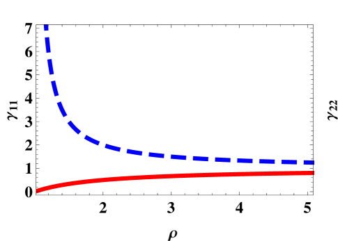
Figure 1: The constitutive parameters $\gamma_{11}$ (red, solid curve) and $\gamma_{22}$ (blue, dashed curve) plotted versus radial distance $\rho$.

The constitutive parameters $\gamma_{11}$ and $\gamma_{22}$ are plotted versus radial distance $\rho$ in Fig. 1. Both constitutive dyadics are obviously positive definite for all $\rho>1$. In the limit $\rho\to 1$, we see that $\gamma_{11}$ becomes null-valued while $\gamma_{22}$ becomes unbounded. On the other hand, both $\gamma_{11}$ and $\gamma_{22}$ rapidly approach unity as $\rho\to\infty$.

In fact, the structure of our proposed cloak is identical to the Tamm medium which represents the exterior region of a (non-spinning) cosmic string [16]. In a geometric-optics study of this Tamm medium, it was demonstrated that the interior of the cosmic string is almost entirely invisible to a distant observer [17]. Furthermore, the similarity between the constitutive relations (1)–(3) and those of the experimentally-realized cloak of Schurig et al. [11] is noted.

3 Ray trajectories

A study of light rays passing through the cloak specified by the constitutive relations (1)–(3) was performed, within the geometric optics regime. As our ray-tracing methodology is described in detail elsewhere [17, 18], only a brief outline is provided here. For a quasi-planewave with relative wavevector $\underline{k}$, the quantity

$$\mathcal{H}=\det\underline{\underline{\gamma}}(\rho)-\underline{k}\cdot\underline{\underline{\gamma}}(\rho)\cdot\underline{k}$$ (4)

represents a suitable Hamiltonian function. With the parameterizations $\underline{r}(\tau)$ and $\underline{k}(\tau)$, ray trajectories are governed by the coupled vector differential equations [19, 20]

$$\left.\begin{array}[]{l}\displaystyle{\frac{d\underline{r}}{d\tau}=\nabla_{\underline{k}}\mathcal{H}\vspace{10pt}}\\ \displaystyle{\frac{d\underline{k}}{d\tau}=-\nabla_{\underline{r}}\mathcal{H}}\end{array}\right\},$$ (5)

with their direction being given by $\nabla_{\underline{k}}\mathcal{H}$, which is aligned with the time-averaged Poynting vector. Standard numerical methods, such as the Runge–Kutta method, can be used to solve the system (5) for $\underline{r}(\tau)$ and $\underline{k}(\tau)$, once appropriate initial conditions $\underline{r}(0)$ and $\underline{k}(0)$ have been specified.

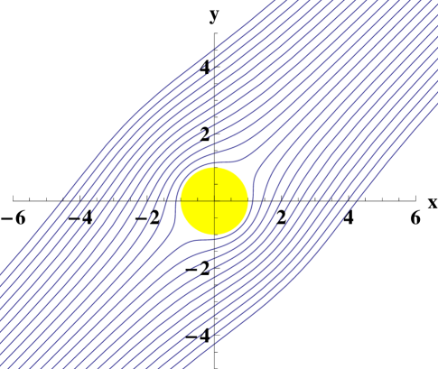
Figure 2: A two-dimensional example of ray trajectories for $\rho_{c}=1.1$. Rays start at equally spaced locations along the line $\underline{x}(0)=\underline{\underline{M}}\cdot\left(30,\nu,0\right)$ with $-12.5<\nu<12.5$ and where the rotation dyadic $\underline{\underline{M}}=\cos\varphi\,\left(\hat{\underline{x}}\,\hat{\underline{x}}+\hat{\underline{y}}\,\hat{\underline{y}}\right)-\sin\varphi\,\left(\hat{\underline{x}}\,\hat{\underline{y}}-\hat{\underline{y}}\,\hat{\underline{x}}\right)$ with $\varphi=\pi/4$; and $\underline{k}(0)$ is directed along $\left(-1,-1,0\right)$.

An example of planar ray trajectories is illustrated in Fig. 2 for $\rho_{c}=1.1$. Yellow shading indicates the disc $\rho=1$. The rays start at equally-spaced locations in the first quadrant of $xy$ plane along a line parallel to $y=-x$, with $\underline{k}(0)$ directed along $\left(-1,-1,0\right)$. The ray trajectories remain in the $xy$ plane. The rays skirt around the outside of the circle $\rho=\rho_{c}$, such that within a few radiuses from the centre of the circle there is minimal deflection of the rays from their original straight line trajectories. Thus the contents of the cloak are almost entirely invisible to a distant observer located in the third quadrant of the $xy$ plane.

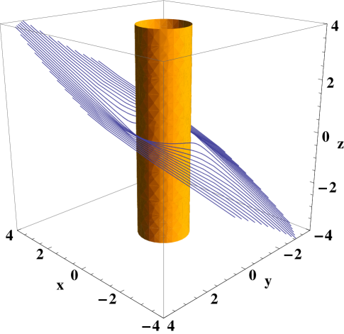
Figure 3: A three-dimensional example of ray trajectories for $\rho_{c}=1.1$. Rays start at equally spaced locations along the line $\underline{x}(0)=\underline{\underline{M}}\cdot\left(30,\nu,29\right)$ with $-12.5<\nu<12.5$ and where the rotation dyadic $\underline{\underline{M}}$ is defined as in Fig. 2; and $\underline{k}(0)$ is directed along $\left(-1,-1,-1\right)$.

An example of ray trajectories in three dimensions is represented in Fig. 3. Here rays start at equally-spaced locations within a plane parallel to $y=-x$ in the octant $\left\{x>0,y>0,z>0\right\}$, with $\underline{k}(0)$ directed along $\left(-1,-1,-1\right)$. The rays do not remain in a single plane in this case, but the deviation from the plane is relatively small, especially at distances beyond a few radiuses from the cloak’s axis.

By considering values of $\rho_{c}$ smaller than $1.1$, the degree of cloaking is improved very little as perceived by an observer more than a few radiuses away from the cloak’s axis. However, by increasing the value of $\rho_{c}$ from $1.1$ the degree of cloaking quite rapidly diminishes.

4 Cloak as a homogenized composite material

Let us now turn to the issue of realizing the cloak specified by the constitutive relations (1)–(3). It was recently demonstrated that certain uniaxial dielectric-magnetic Tamm mediums can be envisaged as homogenized composite materials (HCMs) that can be fabricated from relatively simple component materials [21]. A similar approach is taken here.

Before turning to the homogenization process itself, we must first deal with the inhomogeneity of the proposed cloak. This may be catered for by subdividing the region of space occupied by the cloak into local neighbourhoods which are sufficiently small as to be considered approximately homogeneous. Then the inverse homogenization procedure described later in this section can be applied locally. This piecewise homogeneous approach is documented in detail elsewhere for general Tamm mediums [22].

Now we turn to the homogenization of simple-component composite materials, with our aim being to specify a HCM whose constitutive parameters coincide with the proposed cloak. As our theoretical foundation, we rely on the well-established Bruggeman formalism [23, 24].

Suppose we consider the homogenization of a composite material comprising two isotropic component materials, one being a dielectric-magnetic material with relative permittivity $\epsilon_{a}$ and relative permeability $\mu_{a}$ and the other likewise being a dielectric-magnetic material but with relative permittivity $\epsilon_{b}$ and relative permeability $\mu_{b}$. The component materials $a$ and $b$ are randomly distributed with respective volume fractions $f_{a}$ and $f_{b}=1-f_{a}$. Each component material is distributed as spheroidal particles. The axis of these spheroids for both component materials is assumed to be aligned with the symmetry axis of $\underline{\underline{\gamma}}$, namely the $y$ axis. Thus, the vector

$$\underline{r}_{\,s}=\nu_{\ell}\,\left(\hat{\underline{x}}\,\hat{\underline{x}}+U_{\ell}\,\hat{\underline{y}}\,\hat{\underline{y}}+\hat{\underline{z}}\,\hat{\underline{z}}\right)\cdot\hat{\underline{r}},\qquad\quad\left(\ell=a,b\right),$$ (6)

prescribes the surface of each spheroid relative to its centre. Here the vector $\hat{\underline{r}}$ prescribes the surface of the unit sphere, while the parameter $\nu_{\ell}>0$ is a linear measure of size which is taken to be much smaller than the electromagnetic wavelengths involved. Prolate spheroids are characterized by $U_{\ell}>1$ whereas oblate spheroids are characterized by $U_{\ell}<1$.

In accordance with the Bruggeman formalism, the corresponding HCM is a uniaxial dielectric-magnetic material. Its relative permittivity dyadic $\underline{\underline{\epsilon}}^{Br}$ and relative permeability dyadic $\underline{\underline{\mu}}^{Br}$ have the form

$$\underline{\underline{\tau}}=\tau^{Br}_{11}\left(\hat{\underline{x}}\,\hat{\underline{x}}+\hat{\underline{z}}\,\hat{\underline{z}}\right)+\tau^{Br}_{22}\hat{\underline{y}}\,\hat{\underline{y}},\qquad\left(\tau=\epsilon,\mu\right).$$ (7)

For the case of uniaxial dielectric-magnetic HCMs such as is involved here, full details of the numerical process of computing the dyadics $\underline{\underline{\epsilon}}^{Br}$ and $\underline{\underline{\mu}}^{Br}$ are available elsewhere [21, 23].

Usually, homogenization formalisms are implemented in the forward sense, whereby the constitutive parameters of the HCM are estimated from a knowledge of the constitutive and morphological parameters of their component materials. However, our goal here is to estimate constitutive and morphological parameters of the component materials which give rise to a HCM such that $\epsilon^{Br}_{11}=\mu^{Br}_{11}=\gamma_{11}$ and $\epsilon^{Br}_{22}=\mu^{Br}_{22}=\gamma_{22}$. In order to do so, an inverse implementation of the Bruggeman formalism is required. We note that formal expressions of the inverse Bruggeman formalism have been established [25], but in some instances these formal expressions can be ill-defined [26]. In practice, direct numerical methods may be more effective in implementing the inverse formalism [27]. A note of caution should be added concerning the inverse Bruggeman formalism: certain constitutive parameter regimes have been identified as problematic [28], but these regimes do not overlap with those considered here.

As a representative example, let us focus on a particular inverse homogenization scenario whilst noting that other scenarios are also feasible. For convenience, we seek component materials which are composed of spheroidal particles all of the same shape; i.e., $U_{a}\equiv U_{b}$. Furthermore, we shall assume that the relative permittivity and relative permeability parameters of the component materials are the same; i.e., $\epsilon_{a}\equiv\epsilon_{b}$ and $\mu_{a}\equiv\mu_{b}$. This coincidence of constitutive parameters can be straightforwardly engineered if the component materials themselves are envisaged as HCMs, as has been demonstrated previously [21]. Now, assuming that the relative permittivity and relative permeability of component material $a$ are fixed, we implement the inverse Bruggeman formalism in order to estimate the volume faction, shape parameter and constitutive parameters for component material $b$.

The inversion of the Bruggeman formalism may carried out as follows. Let $\left\{\breve{\epsilon}^{Br}_{11},\breve{\epsilon}^{Br}_{22},\breve{\mu}^{Br}_{11},\breve{\mu}^{Br}_{22}\right\}$ denote the forward Bruggeman estimates of the HCM’s relative permittivity and relative permeability parameters, computed for physically-plausible ranges of the parameters $f_{b}$, $U_{b}$ and $\epsilon_{b}$, namely $f_{b}\in\left(f^{-}_{b},f^{+}_{b}\right)$, $U_{b}\in\left(U^{-}_{b},U^{+}_{b}\right)$ and $\epsilon_{b}\in\left(\epsilon^{-}_{b},\epsilon^{+}_{b}\right)$. Then:

• Fix $U_{b}=\left(U^{-}_{b}+U^{+}_{b}\right)/2$ and $\epsilon_{b}=\left(\epsilon^{-}_{b}+\epsilon^{+}_{b}\right)/2$. For all values of $f_{b}\in\left(f^{-}_{b},f^{+}_{b}\right)$, find the value $f^{\dagger}_{b}$ for which the quantity

  $$\Delta = \left[\left(\frac{\breve{\epsilon}^{Br}_{11}-\gamma_{11}}{\gamma_{11}}\right)^{2}+\left(\frac{\breve{\epsilon}^{Br}_{22}-\gamma_{22}}{\gamma_{22}}\right)^{2}+\left(\frac{\breve{\mu}^{Br}_{11}-\gamma_{11}}{\gamma_{11}}\right)^{2}+\left(\frac{\breve{\mu}^{Br}_{22}-\gamma_{22}}{\gamma_{22}}\right)^{2}\right]^{1/2}$$ (8)

  is minimized.

• Fix $f_{b}=f^{\dagger}_{b}$ and $\epsilon_{b}=\left(\epsilon^{-}_{b}+\epsilon^{+}_{b}\right)/2$. For all values of $U_{b}\in\left(U_{b}^{-},U_{b}^{+}\right)$, find the value $U_{b}^{\dagger}$ for which $\Delta$ is minimized.

• Fix $f_{b}=f^{\dagger}_{b}$ and $U_{b}=U^{\dagger}_{b}$. For all values of $\epsilon_{b}\in\left(\epsilon_{b}^{-},\epsilon_{b}^{+}\right)$, find the value $\epsilon_{b}^{\dagger}$ for which $\Delta$ is minimized.

The steps (i)–(iii) are repeated, using $U_{b}^{\dagger}$ and $\epsilon_{b}^{\dagger}$ as the fixed values of $U_{b}$ and $\epsilon_{b}$ in step (i), and $\epsilon_{b}^{\dagger}$ as the fixed value of $\epsilon_{b}$ in step (ii), until $\Delta$ becomes sufficiently small.

Estimates of $f_{b}$, $U_{b}$ and $\epsilon_{b}$ computed using this scheme are presented in Fig. 4 for the case $\rho_{c}=1.1$. These quantities are plotted versus the radial distance $\rho$. The relative permittivities chosen for component material $a$ were: $\epsilon_{a}=0.01$ for the range $\rho_{c}<\rho\leq 1.5$; $\epsilon_{a}=0.1$ for the range $1.5<\rho\leq 2.5$; and $\epsilon_{a}=0.3$ for the range $2.5<\rho\leq 5$. For all the numerical results presented in Figs. 4, the degree of convergence of the numerical schemes was $<0.1\%$. While the constitutive parameters chosen for component material $a$ are not commonplace, reports of materials with relative permittivities and relative permeabilities close to zero are to be found in the recent literature [29, 30, 31]. Materials with extreme properties are now being considered as well [32]. Furthermore, the constitutive parameters for component material $b$ represented in Fig. 4 are not at all exotic.

5 Closing remarks

We have shown theoretically that the homogenization of a composite material comprising two simple isotropic component materials can result in an HCM which can be used to create a well-functioning cylindrical cloak. By carefully controlling the spheroidal shape of the particles which make up the two component materials, the high degree of HCM anisotropy which is essential for cloaking can be achieved. The inverse Bruggeman formalism provides estimates of the shapes needed for the component particles, as well as their appropriate constitutive parameters and volume fractions. Provided the component materials are weakly dispersive in their constitutive parameters, the proposed cloak can function in a spectral regime of appreciable bandwidth.

The homogenization scenario presented here is by no means the only way of realizing a uniaxial dielectric-magnetic HCM of the required form. For example, the two component materials could both be uniaxial dielectric-magnetic materials (with parallel symmetry axes) which are distributed as spherical particles [33]. Alternatively, four component materials could be homogenized: two isotropic dielectric materials and two isotropic magnetic materials, with all four component materials being composed of spheroidal particles (all with the same alignment) [21]. However, the two-component formulation presented here is more computationally-efficient for the inverse Bruggeman formalism.

Acknowledgment: AL thanks the Charles Godfrey Binder Endowment at Penn State for partial financial support of his research activities.

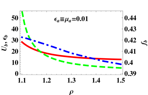
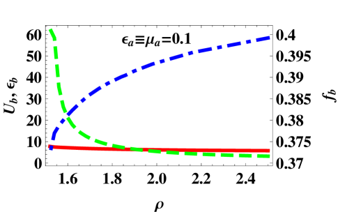
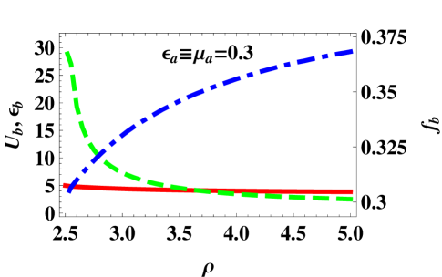
Figure 4: The constitutive parameter $\epsilon_{b}\equiv\mu_{b}$ (red, solid curves), shape parameter $U_{b}\equiv U_{a}$ (green, dashed curves), and the volume faction $f_{b}$ (blue, broken dashed curves) plotted versus radial distance $\rho$ for (a) $\epsilon_{a}\equiv\mu_{a}=0.01$, (b) $\epsilon_{a}\equiv\mu_{a}=0.1$, and (c) $\epsilon_{a}\equiv\mu_{a}=0.3$.

References

- [1] Skrotskii G V 1957 The influence of gravitation on the propagation of light Soviet Phys.–Dokl. 2 226–229
- [2] Plébanski J 1960 Electromagnetic waves in gravitational fields Phys. Rev. 118 1396–1408
- [3] Chandezon J, Dupuis M T, Cornet G and Maystre D 1982 Multicoated gratings: a differential formalism applicable in the entire optical region J. Opt. Soc. Amer. A 72 839–846
- [4] Li L, Chandezon J, Granet G and Plumey J-P 1999 Rigorous and efficient grating-analysis method made easy for optical engineers Appl. Opt. 38 304–313
- [5] Depine R A, Inchaussandague M E and Lakhtakia A 2006 Vector theory of diffraction by gratings made of a uniaxial dielectric-magnetic material exhibiting negative refraction J. Opt. Soc. Amer. B 23 514–528
- [6] Pendry J B, Schurig D and Smith D R 2006 Controlling electromagnetic fields Science 312 1780 2
- [7] Nicorovici N-A P, Milton G W, McPhedran R C and Botten L C 2007 Quasistatic cloaking of two-dimensional polarizable discrete systems by anomalous resonance Opt. Express 15 6314 -6323
- [8] Greenleaf A, Kurylev Y, Lassas M and Uhlmann G 2009 Cloaking devices, electromagnetic wormholes, and transformation optics SIAM Rev. 51 3–33
- [9] Lai Y, Chen H, Zhang Z-Q and Chan C T 2009 Complementary media invisibility cloak that cloaks objects at a distance outside the cloaking shell Phys. Rev. Lett. 102 093901
- [10] Perczel J, Tyc T and Leonhardt U 2011 Invisibility cloaking without superluminal propagation New J. Phys. 13 083007
- [11] Schurig D, Mock J J, Justice B J, Cummer S A, Pendry J B, Starr A F and Smith D R 2006 Metamaterial electromagnetic cloak at microwave frequencies Science 314 977–980
- [12] Smolyaninov I I, Smolyaninova V N, Kildishev A V and Shalaev V M 2009 Anisotropic metamaterials emulated by tapered waveguides: application to optical cloaking Phys. Rev. Lett. 102 213901
- [13] Edwards B, Alù A, Silveirinha M G and Engheta N 2009 Experimental verification of plasmonic cloaking at microwave frequencies with metamaterials Phys. Rev. Lett. 103 153901
- [14] Milton G 2010 Realizability of metamaterials with prescribed electric permittivity and magnetic permeability tensors New J. Phys. 12 033035
- [15] Gao H, Zhang B and Barbastathis G 2011 Photonic cloak made of subwavelength dielectric elliptical rod arrays Opt. Commun. 284 4820–4823
- [16] Mackay T G and Lakhtakia A 2010 Towards a metamaterial simulation of a spinning cosmic string Phys. Lett. A 374 2305–2308
- [17] Anderson T H, Mackay T G and Lakhtakia A 2010 Ray trajectories for a spinning cosmic string and a manifestation of self-cloaking Phys. Lett. A 374 4637–4641
- [18] Anderson T H, Mackay T G and Lakhtakia 2011 Ray trajectories for Alcubierre spacetime J. Opt. 13 055107
- [19] Kline M and Kay I W 1965 Electromagnetic Theory and Geometric Optics (New York: Interscience)
- [20] Sluijter M, De Boer D K and Urbach H P 2009 Ray-optics analysis of inhomogeneous biaxially anisotropic media J. Opt. Soc. Amer. A 26 317–329
- [21] Mackay T G and Lakhtakia A 2011 Towards a realization of Schwarzschild-(anti-)de Sitter spacetime as a particulate metamaterial Phys. Rev. B 83 195424
- [22] Mackay T G, Lakhtakia A and Setiawan S 2005 Gravitation and electromagnetic wave propagation with negative phase velocity New J. Phys. 7 75
- [23] Mackay T G and Lakhtakia A 2010 Electromagnetic Anisotropy and Bianisotropy: A Field Guide (Singapore: Word Scientific)
- [24] Mackay T G 2011 Effective constitutive parameters of linear nanocomposites in the long-wavelength regime J. Nanophoton. (at press)
- [25] Weiglhofer W S 2001 On the inverse homogenization problem of linear composite materials Microw. Opt. Technol. Lett. 28 421–423
- [26] Cherkaev E 2001 Inverse homogenization for evaluation of effective properties of a mixture Inverse Problems 17 1203–1218
- [27] Mackay T G and Lakhtakia A 2010 Determination of constitutive and morphological parameters of columnar thin films by inverse homogenization J. Nanophoton. 4 041535
- [28] Jamaian S S and Mackay T G 2010 On limitations of the Bruggeman formalism for inverse homogenization J. Nanophoton. 4 043510
- [29] Alù A, Silveirinha M, Salandrino A and Engheta N 2007 Epsilon-near-zero metamaterials and electromagnetic sources: Tailoring the radiation phase pattern Phys. Rev. B 75 155410
- [30] Lovat G, Burghignoli P, Capolino F and Jackson D R 2007 Combinations of low/high permittivity and/or permeability substrates for highly directive planar metamaterial antennas IET Microw. Antennas Propagat. 1 177–183
- [31] Navarro-Cía M N, Beruete M, Campillo I and Sorolla M 2011 Enhanced lens by and near-zero metamaterial boosted by extraordinary optical transmission Phys. Rev. B 83 115112
- [32] Sihvola A, Tretyakov S and de Baas A 2007 Metamaterials with extreme material parameters J. Commun. Technol. Electron. 52 986–990
- [33] Mackay T G and Weiglhofer W S 2000 Homogenization of biaxial composite materials: dissipative anisotropic properties J. Opt. A: Pure Appl. Opt. 2 426–432