Analytic solution of the fractional advection diffusion equation for the time-of-flight experiment in a finite geometry

Abstract

A general analytic solution to the fractional advection diffusion equation is obtained in plane parallel geometry. The result is an infinite series of spatial Fourier modes which decay according to the Mittag-Leffler function, which is cast into a simple closed form expression in Laplace space using the Poisson summation theorem. An analytic expression for the current measured in a time-of-flight experiment is derived, and the sum of the slopes of the two respective time regimes on logarithmic axes is demonstrated to be $-2$, in agreement with the well known result for a continuous time random walk model. The sensitivity of current and particle number density to variation of experimentally controlled parameters is investigated in general, and the results applied to analyze selected experimental data.

I Introduction

Modern solid state electronics is largely based upon inorganic, crystalline materials, such as silicon and germanium, the transport properties of which are generally well understood Kittel (1996). The same applies to gaseous electronics, for which there is a one-to-one correspondence with crystalline condensed matter Robson (1985). On the other hand, organic semiconductors are attracting increasing interesting because of their desirable properties, such as transparency, flexibility, and the prospect of economic advantage over inorganic electronics Forrest (2004). Organic materials, which may be amorphous, exhibit electrical properties which are generally qualitatively and quantitatively quite different from inorganic materials Scher et al. (1991). For example, charge carriers in a time-of-flight experiment exhibit long lived, spatially dispersed structures. Furthermore, the roles of the mobility and diffusion coefficients, $\mu$ and $D_{L}$ respectively, are not at all clear cut, as they are in crystalline structures or gases. Such anomalous or “dispersive” behavior arises because the scattering of charge carriers may be accompanied by trapping in localized states for times $\tau$, as determined by a “relaxation function” $\phi(\tau)$, which has an asymptotic time dependence $\sim\tau^{-\gamma}$, with fractional exponent $\gamma$.

The recent interest in “fractional kinetics” derives mainly from the seminal paper of Scher and Montroll Scher and Montroll (1975), whose discussion in terms of a continuous time random walk has spawned an extensive literature in its own right Scher et al. (1991); Compte (1996); Compte and Cáceres (1998); Metzler and Klafter (2000a); Barkai (2001, 2002); Metzler and Klafter (2004). In this literature, it is often assumed that the charge carrier number density $n(z,t)$ may be found as the solution of a fractional diffusion equation, which for present purposes we will refer to as the “Caputo” form of the fractional advection diffusion equation:

$${}_{0}^{C}D_{t}^{\gamma}n+W\frac{\partial n}{\partial z}-D_{L}\frac{\partial^{2}n}{\partial z^{2}}=0,$$ (1)

where ${}_{0}^{C}D_{t}^{\gamma}$ is the Caputo fractional partial derivative with respect to $t$ of order $\gamma$. The Caputo derivative (see Appendix A) accounts for trapping in localized states. This is appropriate for a thin sample of amorphous material confined between two large plane parallel boundaries, with all spatial variation confined to the normal direction, which defines the $z$ axis of a system of coordinates. In addition it is assumed that the small signal limit prevails, and that both the drift velocity $W=\mu E$ , also directed along the $z$ axis, and the longitudinal diffusion coefficient $D_{L}$ derive entirely from an externally applied field $E$. For non-dispersive transport, $\gamma\to 1$ such that ${}_{0}^{C}D_{t}^{\gamma}n\rightarrow\frac{\partial n}{\partial t}$, and Eq. (1) assumes the familiar classical form Huxley and Crompton (1974). The present article focuses on new techniques for solution of Eq. (1) for the purposes of better understanding the factors influencing experiment.

Before proceeding with the detailed analysis, it is important to bear in mind that Eq. (1) is only approximate. Just as the kinetic theory of classical charge carrier transport in crystalline semiconductors and gases has been developed to a sophisticated level through solution of Boltzmann’s kinetic equation, a more general and accurate picture of anomalous transport in amorphous media should be obtained through solution of a fractional kinetic equation in phase space, in which the microscopic collision operator accounts for scattering and trapping processes. Projection onto configuration space is achieved by integration over velocity space, yielding (with approximations) Eq. (1) plus expressions for macroscopic properties such as $\mu$ and $D_{L}$. The phase space approach is beyond the scope of the present work, and the reader is referred to Robson and Blumen (2005) for such considerations.

Whatever the medium, gaseous or condensed matter, crystalline or amorphous, the advection diffusion equation (1) is usually assumed to provide the link between theory and experiment, its limitations not withstanding. Thus, on the one hand, solution of the Boltzmann kinetic equation provides theoretical values of $\mu$ and $D_{L}$, and on the other, solution of Eq. (1) for $n(z,t)$, with appropriate boundary and initial conditions, enables experimental data to be unfolded to furnish empirical values of the same transport properties. Comparison of theoretically derived and experimentally measured transport properties then gives information about the fundamental microscopic nature of the interaction of charge carriers with the medium including the trapping/detrapping process. This procedure is standard for electrons and ion “swarms” in gases Huxley and Crompton (1974), but application of the idea to amorphous media awaits the further development of fractional Boltzmann phase space kinetics. That is part of our long term theoretical program, but in the meantime, we focus in the present article on the more practical imperative of developing an accurate and efficient means of solving Eq. (1).

To this end, a simple and numerically efficient solution of Eq. (1) would be highly desirable. Previously reported solutions of fractional diffusive systems for bounded media have been expressed in terms of infinite series solutions Agrawal (2002); Metzler and Klafter (2000b); Metzler and Klafter (2000a). We show that the series solution to Eq. (1) with absorbing boundaries may be collapsed into a simple closed form solution in Laplace space by building upon the experience gained in solution of the non-dispersive diffusion equation in gaseous electronics, specifically, for the pulsed radiolysis drift tube experiment Robson (1985). The structure of this article is as follows: In Section II, we model the time of flight experiment Tiwari and Greenham (2009) and obtain a formal analytic solution of Eq. (1) as a series of Mittag-Leffler functions, which is cast into a tractable form, suitable for practical purposes, using the Poisson summation theorem. In Section III, we express the current measured in a time-of-flight experiment in terms of this analytic solution, and show analytically that sums of the slopes in distinct time regimes add up to -2 on a log-log plot, as first predicted by Scher and Montroll Scher and Montroll (1975) and as observed in many experiments Scher et al. (1991). In Section IV, we explore the way that current varies with experimental parameters, and go on to fit selected experimental data. We show that our solution demonstrates the power-law decay characteristic of dispersive transport.

II Analytic solutions of the fractional diffusion equation

In this article, we will use Eq. (1) to model a disordered semiconductor in a time of flight experiment Tiwari and Greenham (2009). The relationship between the various forms of the fractional advection diffusion equation using both Caputo and Riemann-Liouville forms of the fractional derivative operator are discussed in Appendix A. A one dimensional equation, such as (1), is appropriate for a thin sample of disordered material confined between two large plane parallel boundaries, which we shall take to be at $z=0$ and $L$ respectively. All spatial variation is confined to the normal direction, which defines the $z$ axis of a system of coordinates. In addition it is assumed that the small signal limit prevails, and that both the drift velocity $W=\mu E$ (where $\mu$ is the mobility) and the longitudinal diffusion coefficient $D_{L}$ derive entirely from an externally applied field $E$.

In the idealized time-of-flight experiment, a sharp pulse of $n_{0}$ charge carriers is released from a source plane $z=z_{0}$ at time $t=t_{0},$ i.e.,

$$n(z,t_{0})=n_{0}\delta(z-z_{0}),$$ (2)

and the fractional advection diffusion equation is solved using the methods and techniques described below. The solution for other experimental arrangements, e.g., for sources distributed in space and/or emitting for finite times, can be found by appropriate integration of this fundamental solution over $z_{0}$ and/or $t_{0}$ respectively. The solution for perfectly absorbing boundaries, for which

$$n(0,t)=0=n(L,t)$$ (3)

is

$$n(z,t)=n_{0}\sum_{m=1}^{\infty}\varphi_{m}(z)E_{\gamma}\left(-\omega_{m}\left(t-t_{0}\right)^{\gamma}\right),$$ (4)

where the spatial modes are

$$\varphi_{m}(z)\equiv\frac{e^{\lambda\left(z-z_{0}\right)}}{L}\left(\cos\left[k_{m}(z-z_{0})\right]-\cos\left[k_{m}(z+z_{0})\right]\right),$$

and where

$$\lambda \equiv\frac{W}{2D_{L}}$$ (5a)

$$\omega_{m} \equiv D_{L}\left(\lambda^{2}+k_{m}^{2}\right)$$ (5b)

$$k_{m} \equiv\frac{m\pi}{L}.$$ (5c)

In Eq. (4), $E_{\gamma}(z)$ is the Mittag-Leffler function of order $\gamma$:

$$E_{\alpha,\beta}(z) \equiv \sum_{k=0}^{\infty}\frac{z^{k}}{\Gamma(\alpha k+\beta)}$$ (6)

$$E_{\alpha}(z) \equiv E_{\alpha,1}(z).$$

Equation (4) gives an exact solution, however, this expression is somewhat difficult to manipulate due to the presence of the Mittag-Leffler function. Furthermore, a large number of terms are needed for this series to converge, and the numerical evaluation of the Mittag-Leffler to suitable precision is computationally difficult.

As is well known, fractional models obey a correspondence principle, where non-fractional behavior is recovered in appropriate limits. In this case, in the limit $\gamma\to 1$ the Mittag-Leffler function reduces to an exponential, i.e. $E_{1}(z)=e^{z}$, and (4) reduces to Eq. (3b) in Ref. Robson (1985). In the classical, non-fractional limit Robson (1985), it was shown that the series convergence could be substantially improved through application of the Poisson summation theorem (PST):

$$\sum_{m=-\infty}^{\infty}f(mT)=\frac{1}{T}\sum_{m=-\infty}^{\infty}F\left(\frac{m}{T}\right),$$ (7)

where $F(k)$ is the Fourier transform of $f(x)$. This article will demonstrate that the PST can also be applied to the fractional advection diffusion equation with similar benefits. Attempting to apply the PST directly to Eq. (4) results in an intractable Fourier transform involving the Mittag-Leffler function. On the other hand, the Mittag-Leffler function has a simple Laplace domain representation. Transformed into Laplace space, Eq. (4) becomes

$$\bar{n}(z,s)=n_{0}\sum_{m=1}^{\infty}\varphi_{m}(z)\frac{s^{\gamma-1}}{s^{\gamma}+\omega_{m}},$$ (8)

where without loss of generality we have taken $t_{0}=0$.

Applying the Poisson summation theorem to Eq. (8) gives the equivalent form

$$\bar{n}(z,s)=\alpha e^{\lambda z}\sum_{m=-\infty}^{\infty}\bigg{[}e^{-\beta\left|2Lm-\left(z-z_{0}\right)\right|}\\ -e^{-\beta\left|2Lm-\left(z+z_{0}\right)\right|}\biggr{]},$$ (9)

where the space-independent parameters $\alpha$ and $\beta$ are defined as

$$\alpha(s) \equiv\frac{n_{0}s^{\gamma-1}e^{-\lambda z_{0}}}{2\sqrt{D_{L}}\sqrt{s^{\gamma}+D_{L}\lambda^{2}}}$$ (10)

$$\beta(s) \equiv\frac{\sqrt{s^{\gamma}+D_{L}\lambda^{2}}}{\sqrt{D_{L}}}.$$ (11)

Simplifying Eq. (9), we obtain the closed form expression

$$\bar{n}(z,s)=\alpha e^{\lambda z}\biggl{[}e^{-\beta|z-z_{0}|}-e^{-\beta|z+z_{0}|}\\ -\frac{4\sinh\left(\beta z\right)\sinh\left(\beta z_{0}\right)}{e^{2\beta L}-1}\biggr{]}.$$ (12)

A necessary condition for convergence to the closed form expression Eq. (12) is

$$|\exp(-2\beta L)|<1,$$ (13)

which defines the region of convergence of the Laplace domain function Eq. (12).

It should be emphasized that Eq. (12) is a general result, valid for fractional and non-fractional cases. For normal transport (i.e., crystalline semiconductors or gaseous electronics), $\gamma=1$, and Eq. (9) has an analytic inverse Laplace transform that reduces to Eq. (7) of Robson (1985), where it was obtained using time domain methods. For dispersive transport, $\gamma<1$, and an analytical inverse Laplace transform is difficult to find, so the applications presented below required numerical inversion of the Laplace transform.

III Currents and the Sum Rule

III.1 Number, number density and charge carrier current in the time of flight experiment

A typical time of flight experiment measures the external current as photogenerated carriers are driven through the sample by an applied electric field. Under the condition that the experimental time scale is much less than the RC time of the measurement circuit, the observed current is the space averaged conduction current

$$I=\frac{1}{L}\int_{0}^{L}j(z,t)dz.$$ (14)

Expressed in terms of the number density $n(z,t)$, the photocurrent is

$$I(t)=q\frac{d}{dt}\left\{\frac{1}{L}\int_{0}^{L}zn(z,t)dz-\int_{0}^{L}n(z,t)dz\right\},$$ (15)

where $q$ is the charge on each carrier. The origin of Eq. (15) is detailed in Appendix B. Substituting the time domain $n(z,t)$ solution Eq. (4) into Eq. (15), the current is found to be

$$I(t)=\sum_{m=1}^{\infty}\kappa_{m}t^{-1}E_{\gamma,0}\left(-\omega_{m}t^{\gamma}\right),$$ (16)

with

$$\kappa_{m}=\frac{2qn_{0}e^{-\lambda z_{0}}k_{m}D_{L}}{L^{2}\omega_{m}^{2}}\sin\left(k_{m}z_{0}\right)\\ \times\left[2\lambda D_{L}\left(e^{\lambda L}\left(-1\right)^{m}-1\right)-L\omega_{m}\right].$$

Alternatively, a closed form expression may be found in Laplace space by substituting Eq. 12 into Eq. (15).

III.2 Sum rule for asymptotic slopes

Experimental time of flight current traces plotted on double logarithmic axes often demonstrate two distinct straight line regimes (see, for example, Figure 5), a distinctive shape which has been described as the “signature” of dispersive transport Scher et al. (1991). In many materials, the sum of the slopes on logarithmic axes of these two regimes is very close to $-2$ (Refs. Scher et al. (1991); Zallen (1983)), a prediction originally made for a continuous time random walk model by Scher and Montroll Scher and Montroll (1975). In what follows, we prove that our expression for the current, Eq. (16), demonstrates the same “sum of slopes” criterion.

The small argument asymptote of the Mittag-Leffler function can be written down from its power series definition, Eq. (6). The result is

$$E_{\gamma,0}(-\omega_{m}t^{\gamma})\sim-\omega_{m}t^{\gamma},$$

where we have neglected terms of order $O\left(\left[\omega_{m}t^{\gamma}\right]^{2}\right)$ and higher. Substituting this into Eq. (16) we find the early time current to be

$$I_{\text{early}}(t) \approx \sum_{m=1}^{\infty}-\kappa_{m}t^{-1}\omega_{m}t^{\gamma}\sim t^{\gamma-1}.$$

Conversely, for the long time current, we use the large $|z|$ asymptote valid for negative real $z$ Gorenflo et al. (2002)

$$E_{\alpha,\beta}(z)=-\sum_{k=1}^{p}\frac{z^{-k}}{\Gamma\left(\beta-\alpha k\right)}+O\left(\left|z\right|^{-1-p}\right).$$

If $t$ is large, then by taking $p=1$ we obtain the following form for the long time current

$$I_{\text{late}}(t) \approx -\sum_{m=1}^{\infty}\kappa_{m}t^{-1}\frac{\left(-\omega_{m}t^{\gamma}\right)^{-1}}{\Gamma\left(-\gamma\right)}$$

$$\sim t^{-(1+\gamma)},\qquad\gamma\neq 1.$$

In summary, the asymptotic forms of the current for $\gamma\neq 1$ are

$$I(t)\sim\begin{cases}t^{-(1-\gamma)},&\text{early times}\\ t^{-(1+\gamma)},&\text{late times},\end{cases}$$ (17)

in agreement with the sums of slopes condition.

It is noteworthy that these asymptotes are independent of the boundary conditions imposed on the system. When solving the fractional diffusion equation $n(z,t)$ is assumed to be factorable as $n(z,t)=Z(z)T(t)$. The time-dependent function, $T(t)$ can be expressed in terms of Mittag-Leffler functions

$$n(z,t)=\sum_{m}Z_{m}(z)E_{\gamma}\left(c_{m}t^{\gamma}\right),$$ (18)

where $c_{m}$ are the separation eigenvalues found by applying the boundary conditions to the differential equation for $Z(z)$. The asymptotes of the Mittag-Leffler functions Gorenflo et al. (2002) are such that physically acceptable solutions must have $c_{m}<0$ so that $n(z,t)$ remains bounded as $t\to\infty$. Imposing only the requirement that the boundary conditions result in a negative separation constant, using Eq. (15) the current must take the form

$$I(t) = \sum_{m}\left\{t^{-1}E_{\gamma,0}\left(c_{m}t^{\gamma}\right)\int_{0}^{L}\left(\frac{z}{L}-1\right)Z_{m}(z)dz\right\}.$$

Using the asymptotic limits detailed above, the time dependence may be brought outside the summation, and the the same temporal asymptotes detailed above then follow. This result is independent of the spatial boundary conditions and hence independent of the specific form of $Z(z)$.

III.3 Transit Time

The transit time can be obtained from the expression for the total number of charge carriers within the medium. Defining

$$\bar{N}(s)\equiv\int_{0}^{L}\bar{n}(z,s)dz$$

we find in Laplace space

$$\bar{N}=\frac{n_{0}}{s}\left[1-e^{-\left(\lambda+\beta\right)z_{0}}-\frac{\sinh\left(\beta z_{0}\right)}{\sinh\left(\beta L\right)}e^{-\lambda z_{0}}\left(e^{\lambda L}-e^{-\beta L}\right)\right].$$ (19)

To simplify the mathematics and obtain an estimate for the transit time, we neglect diffusion by taking the limit $D_{L}\to 0$:

$$\bar{N}_{D_{L}=0} = \frac{n_{0}}{s}\left(1-\exp\left[\frac{-s^{\gamma}\left(L-z_{0}\right)}{W}\right]\right).$$ (20)

In the classical case with $\gamma=1$, the above equation has the expected inverse Laplace transform

$$N_{D_{L}=0}^{(\text{classical})}(t)=n_{0}\left[1-H\left(t-\frac{L-z_{0}}{W}\right)\right],$$

where $H(t)$ is the Heaviside step function.

For the dispersive case, where $\gamma<1$, Laplace inversion by complex contour integration gives

$$N_{D_{L}=0}(t)=n_{0}\sum_{m=1}^{\infty}\eta_{m,\gamma}\left(\frac{L-z_{0}}{Wt^{\gamma}}\right)^{m},$$ (21)

where

$$\eta_{m,\gamma}\equiv\frac{\left(-1\right)^{m+1}\sin\left(m\pi\gamma\right)\Gamma\left(\gamma m\right)}{\pi m!}.$$

In the special case of $\gamma=1/2$, the power series Eq. (21) is equivalent to the closed form expression

$$N_{D_{L}=0}^{(\gamma=0.5)}(t)=n_{0}\,\text{erf}\left(\frac{L-z_{0}}{2W\sqrt{t}}\right),$$ (22)

where erf is the Gaussian error function. It is interesting to note that Eq. (22) demonstrates great dispersion despite it being a zero diffusion limit of the true behavior of the system.

A clear transit time cannot be precisely defined because the packet of charge carriers becomes widely dispersed. Nevertheless, there exist two regimes of current transport behavior, and the boundary between these regimes defines a “transit time” for the material. It can be seen that two distinct regimes will emerge from Eq. (21), according to the magnitude of the term in parenthesis. The transit time, defining the transition between regimes, is therefore approximately given by

$$\frac{L-z_{0}}{Wt_{tr}^{\gamma}}\sim 1.$$

Solving for the transit time $t_{tr}$

$$t_{tr}\sim\left(\frac{L-z_{0}}{W}\right)^{1/\gamma}.$$ (23)

This is in agreement with the expected experimental length and field dependence Scher et al. (1991); Scher and Montroll (1975); Zallen (1983).

Figure 1: (Color online) Impact of the fractional order $\gamma$ on the temporal current profiles. Each curve is the current resulting from the respective number density solution of Figure 2.

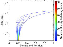
(a) $\gamma=1.00$

(b) $\gamma=0.75$

(c) $\gamma=0.50$

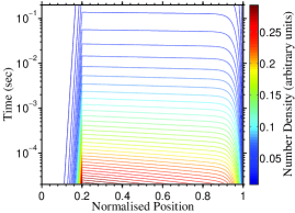
(d) $\gamma=0.25$

Figure 2: (Color online) Impact of the fractional order $\gamma$ of the trapping distribution on the space-time evolution of the number density. In these plots, $W=40/L$ ($\text{s}^{-\gamma}$) and $D_{L}=1/L^{2}$ ($\text{s}^{-\gamma}$).

(a) $W=10.0$; $D_{L}=1.0$

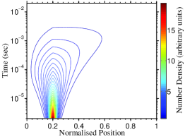
(b) $W=10.0$; $D_{L}=10.0$

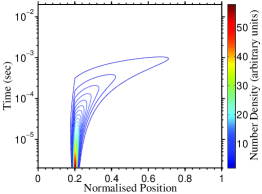
(c) $W=100.0$; $D_{L}=1.0$

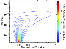
(d) $W=100.0$; $D_{L}=10.0$

Figure 3: (Color online) Space-time evolution of the number density profile for $\gamma=0.8$. Here, $W$ and $D_{L}$ are normalized to the length of the apparatus and are hence both specified in units of $\text{s}^{-\gamma}$.

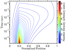
(a) $W=10.0$; $D_{L}=1.0$

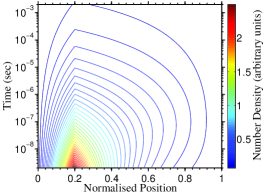
(b) $W=10.0$; $D_{L}=10.0$

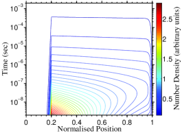
(c) $W=100.0$; $D_{L}=1.0$

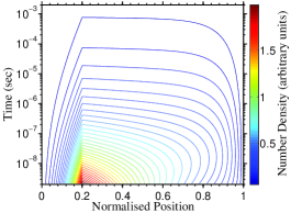
(d) $W=100.0$; $D_{L}=10.0$

Figure 4: (Color online) Space-time evolution of the number density profile for $\gamma=0.4$. Notice that these figures use a different time scale to those in Figure 3. Here, $W$ and $D_{L}$ are normalized to the length of the apparatus and are hence both specified in units of $\text{s}^{-\gamma}$.

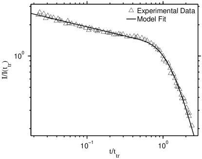
Figure 5: Experimental time of flight current trace data for trinitrofluorenone-polyvinylcarbazole, digitized from Scher and Montroll (1975). The solid line is the model fit.

IV Results

IV.1 Impact of model parameters on the density and current profiles

The model discussed above has five parameters: the fractional drift velocity $W$, the fractional diffusion coefficient $D_{L}$, the fractional order $\gamma$, the initial source location $z_{0}$, and the length of the sample $L$. These parameters are constrained such that $0<\gamma\leq 1$, $0<z_{0}<L$ and $D_{L}>0$. The effects of varying the first three of these parameters will be discussed below. The remaining two, the initial location and length of the sample, have obvious implications for the number density profiles.

IV.1.1 Variation in fractional order $\gamma$

The fractional order $\gamma$ is a dimensionless quantity which defines the degree of the trapping within the medium, with a smaller value corresponding to greater and longer lasting traps. The maximum value of $\gamma=1$ corresponds to “normal transport,” which is governed by the classical (non-fractional) diffusion advection equation.

The impact of $\gamma$ on the electric current is demonstrated in Figure 1. For non-dispersive transport ($\gamma=1$), the result is essentially a time independent (displacement) current until a sharp cutoff where the charged particles exit the system through the electrode. The finite drop off time is a reflection of the diffusion in the system. For dispersive transport, the departure of the current traces from the classical profiles is enhanced as the fractional order decreases. The fractional order $\gamma$ defines the slopes of the two regimes, and hence, characterizes the fundamental shape of the current trace. The relevant relations are given in Eq. (17) above.

Number density profiles corresponding to the aforementioned current solutions are shown in Figure 2. Solutions for $\gamma=1$ exhibit a moving Gaussian “pulse” of charge carriers, spreading according to $D_{L}$ and drifting according to $W$. This is shown in Figure 2a.

For $\gamma<1$, the signature of fractional or dispersive behavior appears. In this mode, the number density profile retains a “memory” of the initial sharp spike at $z=z_{0}$. This peak in the density profile does not drift with $W$, as it does in the non-dispersive case. This long persistence of the initial condition has previously been mentioned in the literature Metzler and Klafter (2000a); Scher and Montroll (1975); Sibatov and Uchaikin (2007). The smaller the value of $\gamma$, the more dispersive the transport. Indeed, for strongly dispersive systems, the spike at $z=z_{0}$ is the most prominent feature of the entire charge distribution for much of its lifetime. This sharp spike is most clearly illustrated in the contour plots of Figures 2c and 2d.

IV.1.2 Impact of the drift velocity $W$ and diffusion coefficient $D_{L}$

The fractional drift velocity has units of $\text{m/\text{s}}^{\gamma}$, and describes the tendency of the charged particles to drift in the positive $z$ direction. The fractional diffusion coefficient has units of $\text{m}^{2}/\text{s}^{\gamma}$, and describes the tendency of the charged particles to diffuse down the concentration gradient. The effects of varying $W$ and $D_{L}$ are demonstrated in Figure 3, for a weakly dispersive system $(\gamma=0.8)$; and in Figure 4 for a strongly dispersive system $(\gamma=0.4)$. The relevant parameters are indicated in the figure captions. For both systems, an increased $W$ sweeps the charge carriers further to the right, and an increased $D_{L}$ spreads the swarm over a wider area.

IV.2 Experimental Results

To demonstrate the process by which this model may be fitted to time-of-flight experimental data, we consider the data for trinitrofluorenone and polyvinylcarbazole (TNF-PVK) presented as Figure 6 of Scher and Montroll (1975). The data was digitized from the scanned plot, and the slopes of the two regimes was used to furnish an estimate for $\gamma$. We used $L=1$ to give a normalized length scale; and selected the initial source location $z_{0}$ to be $0.2$, since the model is largely insensitive to the location of the source, provided it is sufficiently far from the electrodes to avoid substantial “back diffusion.”

The intercept of the two straight lines was taken to be the transit time $t_{tr}$, and the following equation was used to furnish an estimate of W, which provided a starting point for curve fitting:

$$t_{tr}\sim\frac{1}{2}\left(\frac{L-z_{0}}{W}\right)^{\frac{1}{\gamma}},$$ (24)

the factor of $1/2$ being an empirical correction that gives better results when compared with the order of magnitude estimate Eq. (23). The final remaining parameter was initially taken as $D_{L}\approx W/20$.

The parameter estimates discussed above were used as the starting point for nonlinear least squares curve fitting. The Matlab Curve Fitting Toolbox was used. The result of the model fitting is shown in Figure 5.

V Conclusion

We have demonstrated a fractional advection diffusion equation modeling the hopping transport observed in many disordered semiconductors. We have shown that the infinite series of Fourier modes [Eq. (4)] for the bounded solution can be collapsed into a closed form expression using the Poisson summation theorem [Eq. (12)]. It this closed form expression that then facilitates the extraction of model parameters from the experimental data using a simple curve fitting routine. We have modeled a time of flight experiment by assuming the initial condition $n(z,t_{0})=n_{0}\delta(z-z_{0})$. We have calculated the resultant electric current, and shown that the sum of slopes on logarithmic axes is $-2$, as predicted by other models and as verified by experiment. It is possible to extend this solution to sources of finite duration or finite width, by integrating with respect to $t_{0}$ or $z_{0}$, respectively.

Appendix A Caputo and Riemann-Liouville forms of the Fractional Advection Diffusion equation

A.1 Fractional Derivatives

The two forms of fractional derivative commonly used to describe subdiffusive systems are the Caputo derivative and the Riemann-Liouville derivative. In what follows, we describe fractional partial derivatives with respect to $t$ in terms of an arbitrary function $f(t,x,y,...)$. For clarify of presentation, the functional dependence of $f$ on the other variables is suppressed, and we write simply $f(t)$.

The Caputo derivative of order $0<\alpha<1$ is defined as Gorenflo and Mainardi (2008):

$${}_{0}^{C}D_{t}^{\alpha}f(t)\equiv\frac{1}{\Gamma(1-\alpha)}\int_{0}^{t}\left(t-\tau\right)^{-\alpha}f^{\prime}(\tau)d\tau,$$ (25)

where $f^{\prime}(\tau)$ is the ordinary partial derivative $\partial f/\partial t$ evaluated at $t=\tau$. The Laplace transform of the Caputo derivative is:

$$\int_{0}^{\infty}e^{-st}\,{}_{0}^{C}D_{t}^{\alpha}f(t)\,dt=s^{\alpha}\bar{f}(s)-s^{\alpha-1}f(0),$$ (26)

where $\bar{f}(s)$ is the Laplace transform of $f(t)$, and $f(0)$ is the initial condition.

The Riemann-Liouville fractional derivative of order $0<\alpha<1$ is the defined as Gorenflo and Mainardi (2008):

$${}_{0}^{RL}D_{t}^{\alpha}f(t)\equiv\frac{1}{\Gamma(1-\alpha)}\frac{\partial}{\partial t}\int_{0}^{t}\left(t-\tau\right)^{-\alpha}f(\tau)d\tau.$$ (27)

The Laplace transform of a Riemann-Liouville derivative is:

$$\int_{0}^{\infty}e^{-st}\,{}_{0}^{RL}D_{t}^{\alpha}f(t)\,dt=s^{\alpha}\bar{f}(s)-f_{0},$$

where $f_{0}$ is a fractional initial condition:

$$f_{0}\equiv\frac{1}{\Gamma\left(1-\alpha\right)}\lim_{t\to 0}\int_{0}^{t}\frac{f(\tau)}{\left(t-\tau\right)^{\alpha}}d\tau.$$ (28)

A.2 Fractional Advection-Diffusion Equations

The first model for dispersive transport was due to Scher and Montroll Scher and Montroll (1975), who used a continuous time random walk (CTRW) where the waiting time probability density function has divergent mean. A continuous time random walk is characterized by a hopping probability density function (pdf) $\psi(z,t)$. We consider the decoupled case $\psi(z,t)=\lambda(z)w(t)$ where $\lambda(z)$ is the jump length pdf and $w(t)$ is the waiting time pdf. Under these conditions, the CTRW has the Fourier-Laplace space solution Klafter et al. (1987):

$$\bar{n}(k,s)=\frac{1-\bar{w}(s)}{s}\frac{n_{0}(k)}{1-\lambda(k)\bar{w}(s)},$$ (29)

where Fourier transformed functions are denoted by explicit dependence on the Fourier variable $k$, and $n_{0}(k)$ is the Fourier transformed initial condition.

We postulate a CTRW where the waiting time pdf has divergent mean. Such a pdf has the small $s$ asymptote Klafter et al. (1987); Metzler and Klafter (2000a):

$$\bar{w}(s)\sim 1-\left(\tau s\right)^{\gamma}.$$ (30)

We further postulate a well-behaved jump length pdf with moment generating function

$$M_{\lambda}(\chi)=1+M_{1}\chi+\frac{M_{2}\chi^{2}}{2!}+...,$$

for first and second moments $M_{1}$ and $M_{2}$, respectively. This corresponds to a characteristic function (i.e. Fourier transform) in the small $k$ limit of:

$$\lambda(k)=M_{\lambda}(ik)\sim 1+iM_{1}k-\frac{M_{2}k^{2}}{2}.$$ (31)

Substituting these asymptotes into Eq. (29), and discarding terms of order $O(ks^{\gamma})$ and higher, we obtain:

$$\bar{n}(k,s) = \frac{n_{0}(k)s^{\gamma-1}}{s^{\gamma}-iWk+D_{L}k^{2}},$$ (32)

where $W\equiv M_{1}/\tau^{\gamma}$ and $D_{L}\equiv M_{2}/2\tau^{\gamma}$. Equation (32) is the free-space propagator of fractional advection-diffusion. By rearranging Eq. (32), one can derive various forms of fractional advection diffusion equation. For example, one readily obtains:

$$s^{\gamma}\bar{n}(z,s)-s^{\gamma-1}n_{0}(z)+\left(W\frac{\partial}{\partial z}-D_{L}\frac{\partial^{2}}{\partial z^{2}}\right)\bar{n}(z,s)=0,$$ (33)

which is the Laplace transform of the Caputo fractional equation (1). Alternatively, Eq. (32) may be rearranged to give:

$$\bar{n}(z,s)-\frac{n_{0}(z)}{s}+s^{-\gamma}\left(W\frac{\partial}{\partial z}-D_{L}\frac{\partial^{2}}{\partial z^{2}}\right)\bar{n}(z,s)=0,$$ (34)

which is a fractional integral equation. Inverting the Laplace transform in Eq. (34), and taking an ordinary partial derivative with respect to time, one obtains the following form of the fractional advection diffusion equation:

$$\frac{\partial n}{\partial t}+\,_{0}^{RL}D_{t}^{1-\gamma}\left(W\frac{\partial n}{\partial z}-D_{L}\frac{\partial^{2}n}{\partial z^{2}}\right)=0.$$ (35)

Equation (35) is a special case of the fractional Fokker-Planck equation Metzler et al. (1999); Barkai (2001), and is equivalent to the Caputo fractional advection diffusion equation (1) considered in this paper.

Appendix B Derivation of Current Formula

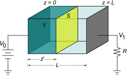
Figure 6: (Color online) Simplified time of flight schematic used in current derivation. The two electrodes at $z=0$ and $z=L$ have potentials $V_{0}$ and $V_{1}$, respectively. A surface $\mathcal{S}$ cuts through the sample at $z=z^{\prime}$; the volume $\mathcal{V}$ is the space between the $z=0$ electrode and the surface $\mathcal{S}$.

Consider a time of flight system where all spatial variation is confined to the $z$ direction, normal to the electrodes. An electrode at $z=0$ is held at a potential $V_{0}$ by an external power supply, and the opposite electrode at $z=L$ has potential $V_{1}$ and is connected via a resistor $R$ to the ground, as shown in Figure 6. We define a surface $\mathcal{S}$ which is normal to the electrodes at a position $z=z^{\prime}$, and a volume $\mathcal{V}$ which is the entire area between the $z=0$ electrode and the surface $\mathcal{S}$.

The overall current will consist of a conduction current and a displacement current. Integrating across the width of the sample:

$$I=\frac{1}{L}\int_{0}^{L}j(z^{\prime},t)dz^{\prime}+\frac{\epsilon A}{L}\frac{d}{dt}\left(V_{0}-V_{1}\right),$$ (36)

where $j(z^{\prime},t)$ is the conduction current passing through the surface $\mathcal{S}$, $\epsilon$ is the permittivity of the semiconducting material, and $A$ is the area of the electrodes.

Under typical measuring conditions, the transit time $t_{tr}$ is much less than the RC time of the circuit. Therefore, we assume that $V_{0}-V_{1}$ is essentially constant, and then the current is simply the space-averaged conduction current:

$$I=\frac{1}{L}\int_{0}^{L}j(z^{\prime},t)dz^{\prime}.$$ (37)

The conduction current leaving the volume $\mathcal{V}$ is the negative rate of change of the charge enclosed:

$$j(z^{\prime},t)=-\frac{d}{dt}\int_{0}^{z^{\prime}}qn(z,t)dz.$$

Using Eq. (37):

$$I = -\frac{q}{L}\frac{d}{dt}\int_{0}^{L}\int_{0}^{z^{\prime}}n(z,t)dzdz^{\prime}.$$

Changing the order of integration:

$$I = -\frac{q}{L}\frac{d}{dt}\int_{0}^{L}\int_{z}^{L}n(z,t)dz^{\prime}dz$$ (38)

$$= -\frac{q}{L}\frac{d}{dt}\int_{0}^{L}\left(L-z\right)n(z,t)dz$$

$$= q\frac{d}{dt}\left\{\frac{1}{L}\int_{0}^{L}zndz-\int_{0}^{L}ndz\right\}.$$

It should be noted that different expressions exist within the literature for the current depending on whether the paper in question uses a multiple trapping model or a hopping model. This is why our current expression (38) is at first glance not equivalent to the current expressions used by some other authors. Under a multiple trapping model, the equivalent is:

$$I(t)\propto\frac{W}{L}\int_{0}^{L}n_{\text{free}}(z,t)dz,$$ (39)

where $n_{\text{free}}$ is the distribution of untrapped particles and $W$ is the drift velocity of these particles. This formula can be obtained by neglecting diffusive flux to substitute $j=Wn_{\text{free}}$ into Eq. (37).

References

- Kittel (1996) C. Kittel, Introduction to Solid State Physics (John Wiley & Sons, New York, 1996), 7th ed., ISBN 0471111813.
- Robson (1985) R. E. Robson, Physical Review A 31, 3492 (1985).
- Forrest (2004) S. Forrest, Nature 428, 911 (2004).
- Scher et al. (1991) H. Scher, M. F. Shlesinger, and J. T. Bendler, Physics Today 44, 26 (1991).
- Scher and Montroll (1975) H. Scher and E. Montroll, Physical Review B 12, 2455 (1975).
- Compte (1996) A. Compte, Physical Review E 53, 4191 (1996).
- Compte and Cáceres (1998) A. Compte and M. O. Cáceres, Physical Review Letters 81, 3140 (1998).
- Metzler and Klafter (2000a) R. Metzler and J. Klafter, Physics Reports 339, 1-77 (2000a).
- Barkai (2001) E. Barkai, Physical Review E 63, 046118 (2001).
- Barkai (2002) E. Barkai, Chemical Physics 284, 13 (2002).
- Metzler and Klafter (2004) R. Metzler and J. Klafter, Journal of Physics A: Mathematical and General 37, R161 (2004).
- Huxley and Crompton (1974) L. G. H. Huxley and R. W. Crompton, The diffusion and drift of electrons in gases (John Wiley and Sons, New York, 1974).
- Robson and Blumen (2005) R. E. Robson and A. Blumen, Physical Review E 71, 061104 (2005).
- Agrawal (2002) O. Agrawal, Nonlinear Dynamics 29, 145 (2002).
- Metzler and Klafter (2000b) R. Metzler and J. Klafter, Physica A: Statistical Mechanics and its Applications 278, 107 (2000b).
- Tiwari and Greenham (2009) S. Tiwari and N. C. Greenham, Optical and Quantum Electronics 41, 69 (2009).
- Zallen (1983) R. Zallen, in The Physics of Amorphous Solids (John Wiley & Sons, 1983), chap. 6, pp. 253–297.
- Gorenflo et al. (2002) R. Gorenflo, J. Loutchko, and Y. Luchko, Fractional Calculus and Applied Analysis 5, 491 (2002).
- Sibatov and Uchaikin (2007) R. T. Sibatov and V. V. Uchaikin, Semiconductors 41, 335 (2007).
- Gorenflo and Mainardi (2008) R. Gorenflo and F. Mainardi, arXiv preprint (2008), eprint 0805.3823, URL http://arxiv.org/abs/0805.3823.
- Klafter et al. (1987) J. Klafter, A. Blumen, and M. F. Shlesinger, Physical Review A 35, 3081 (1987).
- Metzler et al. (1999) R. Metzler, E. Barkai, and J. Klafter, Physical Review Letters 82, 3563 (1999).
- Srigutomo (2006) W. Srigutomo, Gaver-Stehfest algorithm for inverse Laplace transform (2006), URL http://www.mathworks.com/matlabcentral/fileexchange/9987.
- Barrowes (2009) B. Barrowes, Multiple Precision Toolbox for MATLAB (2009), URL http://www.mathworks.com/matlabcentral/fileexchange/6446.