Evolution of Currents of Opposite Signs in the Flare Productive Solar Active Region NOAA 10930

Abstract

Analysis of a time series of high spatial resolution vector magnetograms of the active region NOAA 10930 available from SOT/SP on-board Hinode revealed that there is a mixture of upward and downward currents in the two foot-points of an emerging flux-rope. The flux emergence rate is almost the same in both the polarities. We observe that along with an increase in magnetic flux, the net current in each polarity increases initially for about three days after which it decreases. This net current is characterized by having exactly opposite signs in each polarities while its magnitude remains almost the same most of the time. The decrease of net current in both the polarities is due to the increase of current having a sign opposite to that of the net current. The dominant current, with same sign as the net current, is seen to increase first and then decreases during the major X-class flares. Evolution of non-dominant current appears to be a necessary condition for a flare initiation. The above observations can have a plausible explanation in terms of the superposition of two different force-free states resulting in non-zero Lorentz force in the corona. This Lorentz force then push the coronal plasma and might facilitate the magnetic reconnection required for flares. Also, the evolution of the net current is found to follow the evolution of magnetic shear at the polarity inversion line.

1 INTRODUCTION

The magnetic field in sunspots has been studied with increasing details ever since Hale’s first detection (Hale, 1908). With the advent of vector magnetographs, it is now possible to estimate few components of the competing electrodynamic forces (Borrero, Lites & Solanki, 2008; Venkatakrishnan & Tiwari, 2010) which had been invoked to define the sunspot structure and equilibrium (Chitre, 1963; Mayer, Schmidt & Weiss, 1977; Parker, 1979; Low, 1984). An important electrodynamic quantity in this context is the electric current which is expected to play a crucial role in eruptive processes (Melrose, 1991; Longcope & Welsch, 2000). Such currents in astrophysical plasmas are generally produced by deforming magnetic field through the motion of the plasma in which the field is embedded (Parker, 1979). The sites of these deformations could be either the convection zone (Fan, 2009; Longcope, Fisher & Pevtsov, 1998) with subsequent emergence of the deformed fields (Leka, Canfield, McClymont & van Driel-Gesztelyi, 1996) or the photosphere (Aulanier, Démoulin, & Grappin, 2005).

A classic case of flux emergence was seen in the active region NOAA 10930 which has been well studied for a variety of flare related magnetic phenomena. Although, the emergence of current carrying fine structures were reported (Lim, Chae, Jing, Wang & Weigelmann, 2010; Wang, Jing, Tan, Weigelmann & Kubo, 2008), there has been so far no study of the evolution of the net current in this region. Such a study is important because of the highly flare productive nature of this active region. In this paper, we follow the time evolution of the net vertical current in the whole active region spanning two major X-class flares and show some new properties of current-bearing flux emergence that seem to be relevant for the triggering of the flares.

2 OBSERVATIONAL DATA AND ITS PROCESSING

The Spectro-Polarimeter (Tsuneta et al., 2008; Suematsu et al., 2008; Ichimoto et al., 2008) on board HINODE (Kosugi et al., 2007) satellite makes spectro-polarimetric measurements at a spatial sampling of 0.3^′′. The I, Q, U and V Stokes profiles have been obtained in 6301.5 Å and 6302.5 Å lines. The spectro-polarimeter makes the maps of the Stokes vector by scanning the slit across the active regions. The spatial sampling is 0.295${}^{\prime\prime}~{}{\rm{pixel}}^{-1}$ along the slit direction and is 0.317${}^{\prime\prime}~{}{\rm{pixel}^{-1}}$ in the scanning direction. There are many modes of observations depending on the exposure time, resolution, signal-to-noise ratio etc. We have obtained the data of AR NOAA 10930 in fast mapping mode. The Stokes signals are calibrated using the standard solar software pipeline for the spectro-polarimetry. The complete information on the vector magnetic fields is obtained by inverting the Stokes vector using the Milne Eddington inversion (Skumanich & Lites, 1987; Lites & Skumanich, 1990; Lites et al., 1993). The ambiguity in the transverse field is resolved based on the minimum energy algorithm developed by Metcalf (1994) and implemented in FORTRAN by Leka, Barnes & Crouch (2009). The magnetic field vector has been transformed to the disk center using the method described in Venkatakrishnan, Hagyard, & Hathaway (1989). The resulting vertical (B_z) and transverse (B_t) magnetic fields have measurement errors of 8 G and 23 G respectively.

The horizontal components of the magnetic fields B_x and B_y are utilized in computing the vertical current density $J_{z}$ as

$$J_{z}=\frac{1}{\mu}(\frac{\partial B_{y}}{\partial x}-\frac{\partial B_{x}}{\partial y})~{}~{}~{},$$ (1)

where $\mu$ is the magnetic permeability.

We computed the net current in the active region separately for the N and S polarity regions by integrating the current density over the surface. This has been done only for those pixels whose B_z value is larger than 50 G to avoid the noisy pixels and the pixels that do not belong to the active region.

3 RESULTS

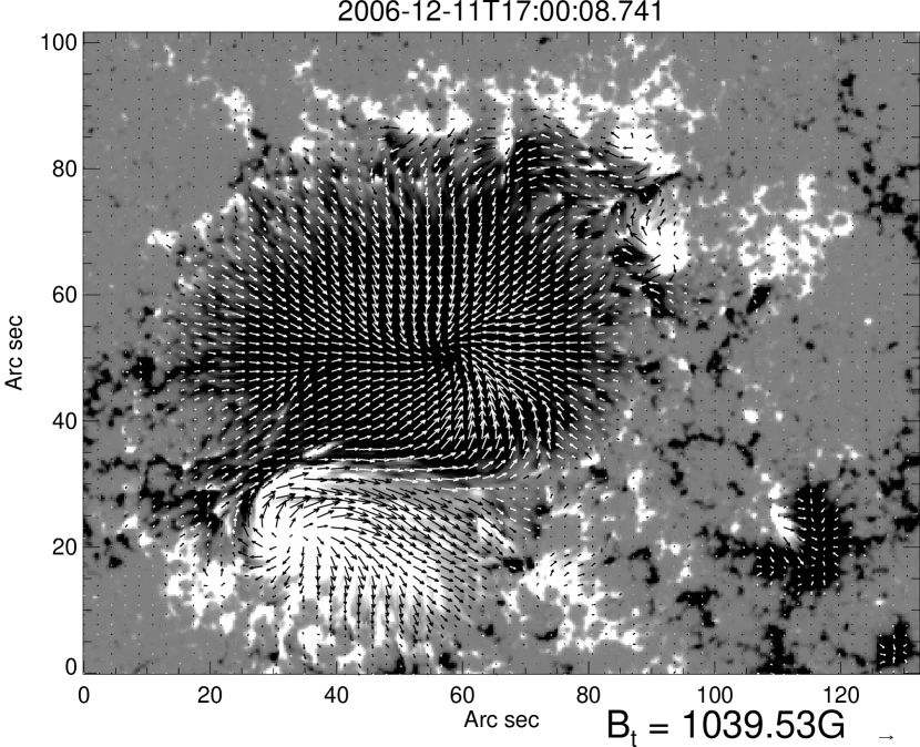
Figure 1: A sample vector magnetogram showing the ambiguity resolved transverse field overlaid upon the vertical magnetic field. The black (white) color represents the S (N) polarity regions. Arrows indicate the direction of the transverse magnetic fields.

Figure 2: Evolution of flux ($+$ symbol) in North (top) and South (bottom) polarities is plotted as a function of time. The small dashed lines represent the linear least square fit to the data points. The net vertical current ($\times$ symbol) in each of these polarities is shown in the same plot. The negative(positive) net vertical current is observed in the North(South) polarity spot. The Y-axis on the right side is shown for the net currents. The long vertical lines represent the on-set time of X3.4 and X1.3 class flares. The $\times$ symbol with vertical bar shown on the top plot in the left hand side is error in measuring the net current.

Figure 1 shows a sample vector magnetogram of the active region NOAA 10930. Both, N-polarity and S-polarity sunspots are present in the active region. The S-polarity sunspot is large and well developed. The N-polarity sunspot is small and emerging. The transverse field vectors are highly sheared near the polarity inversion lines (PIL). Figure 2 shows the temporal evolution of magnetic flux of N and S-polarity regions over a period of 6 days. The flux has been estimated for those pixels whose vertical magnetic field strength is larger than 50 G. The flux is observed to increase from the beginning of the observations till the end of December 12 and after that no flux emergence is seen up to the middle of December 14. This is followed by a small flux emergence before the X1.3 class flare followed by a decrease in flux. Since we have used the pixels where B_z values are larger than 6 times the measurement error, the error in flux computation is negligible. The flux increased linearly from December 9 till the end of December 12 at a rate of about 0.6$\times$10²⁰ Mx h^-1 in both the polarities. This indicates the emergence of a flux rope with end points in the N and S-polarity of this active region.

3.1 Spatial Map of Vertical Current Density

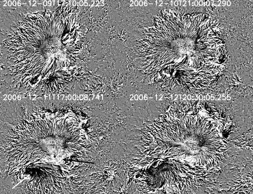
Figure 3: Maps of vertical current density obtained at different time of the epoch. The black and white arrows in the bottom left figure show the dominant regions of vertical current density in two different polarities. The field-of-view of each map is same as in Figure 1.

Figure 4: Histogram of the vertical current density of full map. The values of current density extended till 200 mA $m^{-2}$ in both the positive and negative side.

Figure 3 shows the spatial maps of vertical current densities at different epochs. It also shows how the distribution of current densities in spatial locations evolve in time. The current density is of mixed sign (salt and pepper) in the umbra of S-polarity sunspot while it is in the form of fibrils in the penumbra, alternatively changing their sign azimuthally as has been reported by Su, Sakurai & Suematsu (2009) and Tiwari, Venkatakrishnan, & Sankarasubramanian (2009). Apart from these there is a region of dominant sign of current density in the S and N-polarity regions. In the S-polarity region the positive current density is dominant and in the N-polarity region the negative current density is dominant. These regions are shown by arrows in both the polarities (Figure 3 bottom left). These dominant regions grow with time. They occupy a portion of the umbra and also extend to the penumbra in both polarities. The vertical current density is distributed over a wide range of magnitudes. Figure 4 shows the histogram of the vertical current density in the active region. The plot shows that positive as well as negative current densities exist in the active region and its tail is extended up to $\pm 200~{}mA~{}m^{-2}$. The amplitude of variation of the vertical current density on small scales is comparable to that seen in the less flare productive region 10933 by Venkatakrishnan & Tiwari (2009).

3.2 Temporal Evolution of Net Vertical Current Over The Active Region

In order to examine the temporal evolution of net vertical currents in different polarity regions, we isolated the N and S-polarity regions by using a threshold of 50 G in the vertical magnetic field strength. We then integrated the currents for the N and S-polarity regions separately. Figure 2 shows the net current over the N (bottom) and S-polarity (top) regions. The net current evolution is plotted over the flux evolution to compare the both. The negative (positive) net current is represented as I_n (I_p), which is observed to be dominant in N (S) polarity region. The integrated currents in each polarity is expressed in terms of Amps. We used the histogram depicted in Figure 4 to arrive at a measure of the statistical uncertainty of average vertical current density as $\delta J_{z}=\sigma_{J_{z}}/\sqrt{(}N)$ (Hagino & Sakurai, 2004), where, $\sigma_{J_{z}}$ is the FWHM of the histogram and N is the number of data points. From this, we estimated the statistical uncertainty in the integrated net current as $\delta I=\sqrt{(}N)\cdot\sigma_{J_{z}}\cdot\Delta S$ with $\Delta S$ being the area of each pixel in m² (since, $I=\sum\limits_{N}J\cdot\Delta S$). The uncertainty in measuring the net current is shown in the top left hand side of the Figure 2. Initially, the current is small till December 10, 2006. Later, it increased linearly in both the polarities till mid of December 11, 2006. This part of the net current increase just follows the curve of increase in flux (see the plot Figure 2). Later it undulates for a few hours and then starts decreasing till the end of observations. The behavior of currents is almost the same in both the polarities throughout the observations. The dashed vertical lines mark the times of the peak flux of the X3.4 and X1.3 class flare that occurred on Dec 13 and 14 respectively. After the X3.4 class flare, there is a decrease in net current in both the polarities, however after the X1.3 class flare the net current increased by a small amount in both the polarities.

Figure 5: Left: The temporal evolution of net vertical currents in S-polarity region (shown by $+$ symbol). Right: Same as left side plot but for N-polarity region. The top and bottom plots show the temporal evolution of positive and negative currents in the same polarity region. The right side scale on the Y-axis is drawn to show the I_abs in each of the polarities. The I_abs is shown by $\times$ symbol.

From the flux evolution map (Figure 2) it is clear that there is an increase in flux and the net current till the beginning of Dec 12. However, the net current started to decrease after the beginning of December 12, even as the flux continued to emerge. In order to seek an answer to this puzzle we examined the vertical current of both the signs in each polarity region separately. Figures 5(left) and (right) show the vertical currents for the S and N-polarity regions. Let IN(+), IN(-), IS(+) and IS(-) denote the positive (+) and negative (-) currents in the North(N) and South (S) polarity regions. The following observations are then of particular importance.

• IS(+) increased till Dec 12.5 by about 1.3$\times$10¹³ Amps, decreased till Dec 13.6 by about 0.5$\times$10¹³ Amps, increased again till Dec 14.5 by about 0.5$\times$10¹³ Amps then decreased till X1.3 class flare by about 0.2$\times$10¹³ Amps, followed by a slight increase in its value. At the same time the IS(-) was almost constant at 2.2$\times$10¹³ Amps with small increase in its value till December 12.5 by about 0.5$\times$10¹³ Amps. Later, it decreased till the on-set of X3.4 class flare by about 0.3$\times$10¹³ Amps and then increased again till 14.5 by about 0.6$\times$10¹³ Amps then decreased till X1.3 class flare. The pattern of increase and decrease in IS(+) and IS(-) coincides well from Dec 11 till the onset of X3.4 class flare. Then onwards IS(-) increased and and IS(+) decreased till the on-set of X1.3 class flare. After this IS(-) decreased and IS(+) increased in magnitude slightly.

• IN(-) increased till Dec 12.5 (with a change in rate of increase after 11.3) by about 1.5$\times$10¹³ Amps, decreased till X1.3 class flare by a small amount of about 0.5$\times$10¹³ Amps, followed by a slight increase. On the other hand, IN(+) increased till Dec 12.5 (with undulations), decreased till 13.3, increased again till 14.5 then decreases till X1.3 class flare.

• There is a mis-match in the values of the dominant current and non-dominant current at least by a factor of about 1.5 at all the time.

• The most important feature observed is that the dominant current appears to follow the flux evolution in each polarities whereas the non dominant current evolves differently.

The above observations then suggest that increase of dominant and non-dominant current could be due to both emergence and deforming flows, while decrease in both types of currents can be either due to deforming flows or diffusion of field (we rule out the later process in section 4). We have noted that increase in dominant current by and large follows the flux emergence, while increase in non-dominant current does not follow the flux evolution so closely, except in the beginning. The increase in non-dominant current is the reason for decrease in the net current as depicted in Figure 2. The small decrease in IS(-) and IN(+) on Dec 11 between 0 to 7 hrs could be related to the C-class flares observed by GOES satellite (cf. Figure 1(a) of Tiwari, Venkatakrishnan, & Gosain (2010)). The increase in the opposite current leads to decrease in the net current in both the magnetic polarities after beginning of December 12.

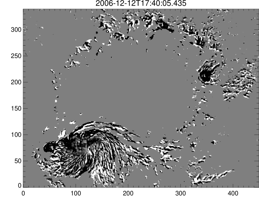
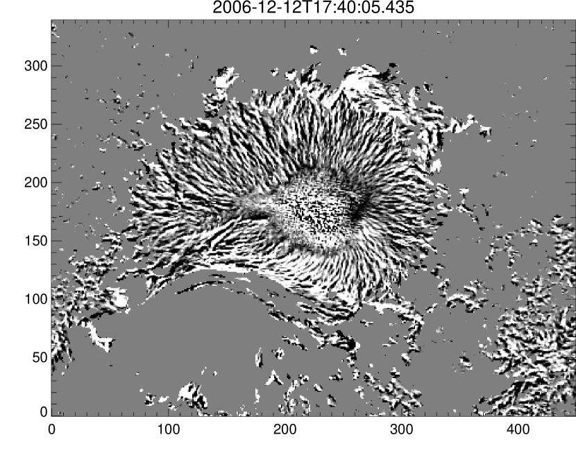
Figure 6: Maps of vertical current density used to compute the net vertical current in the N (left) and S (right) polarity regions in the active region.

Figure 6 (left and right) shows a map of the current densities which are utilized in computing the currents of different polarity regions in Figure 5 (left and right). The left side image shows the map of positive and negative currents for the N-polarity region. The right side is for the S-polarity region. The map shows that the majority of the current originates from the dominant current region which is large in size and the opposite current originates from the smaller size regions, for example the salt and pepper like region in the umbra and fibril type regions in the penumbra.

Figure 5 also shows the sum of absolute value of net current of both signs (${I_{abs}}$), obtained in N and S-polarity regions. For comparisons with the dominant current in each polarity we have shown the ${I_{abs}}$ separately in IS and IN. The ${I_{abs}}$ in the north polarity is shown as negative. This is simply to compare it with the dominant current. The plot shows that ${I_{abs}}$ in the N-polarity sunspot increases with time in the beginning and reaches almost a plateau in later part of the observations. In the S-polarity region, ${I_{abs}}$ increased till the mid of December 12, decreased thereafter till mid of December 13 and then it increased. ${I_{abs}}$ in the S-polarity increased up to about 6$\times$10¹³ Amps. There is a mis-match in the values of ${I_{abs}}$ in the N and S-polarity regions. ${I_{abs}}$ is large in the S-polarity region compared to the N-polarity region. This is not unreasonable because the S-polarity carries a larger amount of flux than the N-polarity spot. The pattern of evolution of ${I_{abs}}$ in both the polarities is following the dominant current, however their magnitudes are different.

4 SUMMARY AND DISCUSSION

Active region NOAA 10930 is a flare productive region and it produced several X and M-class flares during its disk passage. The active region was associated with an emerging flux. Several morphological details of the flux emergence have already been reported (Kubo et al., 2007). In our present work, we note that although there is a flux imbalance in the active region, the rate of flux emergence is the same in both the polarities. The vector field maps showed that the transverse field in the N-polarity region was highly sheared near the PIL and there was a twisted flux rope emergence (Schrijver et al., 2008). The flux was continuously increasing till the end of Dec 12 and there after it leveled off till December 14, followed by a smaller bout of emergence till 15th. The net current, I_n & I_p in each polarity also increased over a couple of days and then it started decreasing. The decrease in the net current can be attributed to the fact that the opposite current in the same polarity region was also increasing with time. For example in the S-polarity region the positive current IS(+) was the dominant one and the IS(+) increased till end of Dec 12. Meanwhile, the opposite current, IS(-) started increasing after beginning of Dec 12. A similar behavior was also found in the N-polarity region. This clearly shows that the emerging flux carries the dominant current. However, the the different behaviour of the non-dominant current suggests that mostly it is related to the deforming motion of the flux tube but partly related to the emergence. Since the sign of current relative to the sign of flux indicates the chirality of the current, this means that the emerging flux and deforming flows produces both types of chirality of the current. If the origin of the chirality lies in the vorticity of the sub-photospheric flows that distort the magnetic field, then it shows that both signs of vorticity exist in the sub-surface flows. However, it must be noted here that the observed opposite current might have nothing to do with the surface or shunt current which is required by Parker (1996) to neutralize the photospheric current for creating the field free regions outside the sunspot.

Let us now see whether the evolution of current is related to the flares. The evolution of the current with dominant sign (IS(+) and IN(-)) in each polarity (Figure 5) is seen to decrease during the period from December 13 to 14, which corresponds to the period when two X-class flares occurred. The decrease of current of a given sign (IS(+) and IN(-)) cannot be attributed to the emergence of opposite current, as was done to explain the decrease of the net current (I_n and I_p). Currents can decrease either by ohmic dissipation or by deformation of the magnetic field because of plasma motion on a dynamical time scale. The time scale for this deformation is then the Alfv́en travel time across the active region. Given the size of 60 arc-sec and Alfv́en speed of 10 km s^-1 in the photosphere, the Alfv́en travel time works out to be of the order of 1 hour. This is smaller than the cadence of the vector magnetograms. Hence one can admit the possibility of the dynamical deformation of the field, which can then explain the observed decrease of the current. In summary, the increase in current can be attributed to emergence, while the decrease in current on time scales smaller than the diffusive time can only be attributed to the dynamical deformation of the magnetic field. It is possible that the flare could have been triggered due to such a dynamical evolution. In fact, indirect evidence for such a dynamical process associated with the December 13, X3.4 class flare, was found from the high cadence G-band pictures (Gosain, Venkatakrishnan, & Tiwari, 2009). It may be noted that the current with the non-dominant (IS(-) and IN(+)) sign showed episodes of decrease before the X-class flares. Except IN(-), all components of the current increased for some time before each flare and then decreased. IN(-) showed no increase before the X1.3 class flare. The dynamical evolution of magnetic field alone cannot lead to an eruption but it also needs triggering by reconnection for that. Reconnection, in turn, requires pushing two oppositely directed magnetic field lines towards each other to a viable limit such that the magnetic field becomes discontinuous and the small-scale effects become dominant. Because of the complex dynamics of the plasma, it is unlikely that this discontinuity will form at the very beginning of the evolution phase which explains the existence of a time delay between the onset of the evolution and the X-ray flare peak. However, we believe that it would be very difficult to predict the onset of the flare purely from a study of the photospheric magnetic field.

The emergence of dominant current (IS(+) and IN(-)) may not be a sufficient condition for the flare. It is seen at least in this active region that flare occurs only after a significant evolution of non-dominant current. This is true for both the X3.4 and X1.3 class flare. A similar behavior is found in the case of magnetic helicity by Park et al. (2010), wherein it is observed that injection of opposite sign of helicity triggers the X3.4 class flare. So, maybe the non-dominant current provides the trigger. In the corona, the field is believed to be force-free. To initiate a flare, the newly emerged field lines have to be pushed against the pre-existing field to produce a current sheet followed by reconnection. So, there has to be some force created on the plasma to push the frozen field. Since plasma forces are not strong enough in the low beta coronal plasma, the only force available is the Lorentz force. But the Lorentz force is possible only in a non-force-free field. It can be shown that the superposition of two force-free fields can result in a non-zero Lorentz force (Appendix). The necessary conditions for this are that a) the new field must have a force-free parameter alpha which is different from that of the pre-existing field AND b) the new field is not aligned with the old field. The larger the amount of new field with different alpha, the larger will be the Lorentz force. This could explain our observation that the major flares occurred only after significant appearance of the oppositely directed current.

The total absolute current increased till the mid of December 12. Since the larger magnitude of current implies the larger value of free magnetic energy, this behavior of the absolute current suggests that the free energy increased till mid of December 12. The current decreased from middle of December 12 suggesting a drop in free energy. The drop in total absolute current in the S-polarity region started well before the beginning of the X3.4 class flare, while it dropped in N-polarity region after the flare . The decrease in total absolute current indicates that the free energy for the flare and CME was supplied from this active region as suggested by Ravindra & Howard (2010), although there is a time delay between the start of decrease in free energy as observed at the photosphere and the release of this energy to the flare and the CME. Once again, we wish to point out that monitoring the free energy in the photosphere might not reveal the exact process of the delivery of this free energy to the flare and the CME. The non linear force free field (NLFFF) analysis of the Hinode vector magnetograms by Schrijver et al. (2008) also suggest that the flares are associated with the energy carried by the currents that originate from the sub photospheric surface.

There is yet another important result seen in these observations. We find that the net observed current within an individual spot evolves from a small value at the beginning of the flux emergence, peaks to a high value, and then diminishes to the pre-emergence values following a decrease in the rate of flux emergence. The net vertical current (I_n and I_p) in both the polarities behaved exactly opposite to each other. Even the magnitude of net current in both the polarities is almost the same throughout the observations. The temporal evolution plot of the current clearly indicated that in one polarity the current was flowing in to the corona and in the other polarity it was returning back to the photosphere. This kind of behavior of evolution of net vertical current is not reported earlier. An inspection of Figure 1 shows that the transverse field was highly sheared at the polarity inversion line (PIL) and not sheared at other locations of the outer penumbra of each spot. Thus, a line integral of the transverse field along a contour at the periphery of each spot would be dominant contributions only from the PIL. Thus, the net current in the interior of this contour would be largely determined by the magnitude of the shear along the PIL. Also, the sign of the current for the contour integral around the S polarity spot would be opposite to that around the N polarity spot. Thus, we can understand the symmetrical evolution of the currents in Figure 2 as chiefly due to the evolution of shear in the PIL of the active region. This is also consistent with the evolution of the mean weighted shear angle (MWSA) of AR 10930 as seen in Figure 3(a) of Tiwari, Venkatakrishnan, & Gosain (2010). Thus, it could well be that the contrasting results on net current obtained in earlier observations (Leka, Canfield, McClymont & van Driel-Gesztelyi, 1996; Wheatland, 2000; Venkatakrishnan & Tiwari, 2009) might be due to observations of the active regions at different stages in the flux emergence and directly related to the magnitude of shear at the PIL. This conjecture can be easily tested with other cases of flux emergence where a time series of vector magnetograms is available. Another interesting extension of this conjecture would be that the emergence of bi-directional currents might also be the cause of the large scatter in the observed chirality of the active regions (Pevtsov, Canfield & Metcalf, 1995), since the average chirality could be affected by presence of a time dependent contribution from flux with opposite chirality. This points to the importance of future synoptic observations of vector magnetic fields of active regions obtained with adequate cadence to eliminate the possible effects of improper sampling of an essentially time-dependent phenomenon. Given the small dynamical time scale for field relaxation, it is essential that the spatial and spectral scanning of an active region be completed well within this time scale. From this point of view, the vector magnetograms from HMI (Schou, Borrero, Norton, Tomczyk, Elmore & Card, 2010) on-board SDO are eagerly awaited.

References

- Aulanier, Démoulin, & Grappin (2005) Aulanier, G. Démoulin, P. & Grappin, R. 2005, A&A, 430, 1067
- Borrero, Lites & Solanki (2008) Borrero, J. M. Lites, B. W. & Solanki, S. K. 2008, A&A, 481, L13
- Chitre (1963) Chitre, S. M. 1963, MNRAS, 126, 431
- Fan (2009) Fan Y., 2009, ApJ, 697, 1529
- Gosain, Venkatakrishnan, & Tiwari (2009) Gosain, S., Venkatakrishnan, P. & Tiwari, S. K., 2009, ApJ, 706, L240.
- Hagino & Sakurai (2004) Hagino, M & Sakurai, T. 2004, PASJ, 56, 831
- Hale (1908) Hale, G. E. 1908, ApJ, 28, 315
- Ichimoto et al. (2008) Ichimoto, K., et al. 2008, Sol. Phys., 249, 233
- Kosugi et al. (2007) Kosugi, T., et al. 2007, Sol. Phys., 243, 3
- Kubo et al. (2007) Kubo, M. et al. 2007, PASJ, 59, S779
- Leka, Canfield, McClymont & van Driel-Gesztelyi (1996) Leka, K. D., canfield, R. C., McClymont, A. N., & van Driel-Gesztelyi L., 1996, ApJ, 462, 547
- Leka, Barnes & Crouch (2009) Leka, K. D., Barnes, G. & Crouch, A. 2009, \aspc, 415, 365
- Lim, Chae, Jing, Wang & Weigelmann (2010) Lim, E., Chae J., Jing J., Wang, H. & Weigelmann, T, 2010, ApJ, 719, 403.
- Lites & Skumanich (1990) Lites, B. W., & Skumanich, A. 1990, ApJ, 348, 747
- Lites et al. (1993) Lites, B. W., Elmore, D. F., Seagraves, P., & Skumanich, A. P. 1993, ApJ, 418, 928
- Longcope & Welsch (2000) Longcope, D. W. & Welsch, B. T. 2000, ApJ, 545, 1089
- Longcope, Fisher & Pevtsov (1998) Longcope, D. W., Fisher, G. H. & Pevtsov, A. A. 1998, ApJ, 507, 417
- Low (1984) Low, B. C. 1984, ApJ, 277, 415
- Mayer, Schmidt & Weiss (1977) Meyer, F., Schmidt, H. U., & Weiss, N. O. 1977, MNRAS, 179, 741
- Melrose (1991) Melrose, D. B. 1991, ApJ, 381, 306
- Metcalf (1994) Metcalf, T. R. 1994, Sol. Phys., 155, 235
- Park et al. (2010) Park, S. H., Chae, J., Jing, J., Tan, C., Wang, H. 2010, ApJ, 720, 1102.
- Parker (1979) Parker, E. N. 1979, “Cosmical magnetic fields: Their origin and their activity” (Oxford, Clarendon Press, New York, Oxford University Press, 1979)
- Parker (1996) Parker, E. N. 1996, ApJ, 471, 485
- Pevtsov, Canfield & Metcalf (1995) Pevtsov, A. A., Canfield, R C. & Metcalf, T. R. 1995, ApJ, 440, L109
- Ravindra & Howard (2010) Ravindra, B. & Howard, T. A., 2010, \basi, 38, 147.
- Schou, Borrero, Norton, Tomczyk, Elmore & Card (2010) Schou, J., Borrero, J. M., Norton, A. A., Tomczyk, S., Elmore, D., Card, G. L., 2010, Sol. Phys., 177, in Press
- Schrijver et al. (2008) Schrijver, C J., DeRosa, M. L., Metcalf, T. et al. 2008, ApJ, 675, 1637
- Skumanich & Lites (1987) Skumanich, A., & Lites, B. W. 1987, ApJ, 322, 473
- Solanki,Rueedi & Livingston (1992) Solanki, S. K., Rueedi, I. & Livingston, W. 1992, A&A, 263, 229
- Su, Sakurai & Suematsu (2009) Su, J. T., Sakurai, T., Suematsu, Y., Hagino, M. & Liu, Y. 2009, ApJ, 697, 103
- Suematsu et al. (2008) Suematsu, Y., et al. 2008, Sol. Phys., 249, 197
- Tiwari, Venkatakrishnan, & Sankarasubramanian (2009) Tiwari, S. K., Venkatakrishnan, P. & Sankarasubramanian, K. 2009, ApJ, 702, 133
- Tiwari, Venkatakrishnan, & Gosain (2010) Tiwari, S. K., Venkatakrishnan, P. & Gosain, S. 2010, ApJ, 721, 622
- Tsuneta et al. (2008) Tsuneta, S., et al. 2008, Sol. Phys., 249, 167
- Venkatakrishnan, Hagyard, & Hathaway (1989) Venkatakrishnan, P., Hagyard, M. J., Hathaway, D. H., 1989, Sol. Phys., 122, 215
- Venkatakrishnan & Tiwari (2009) Venkatakrishnan, P. & Tiwari, S. K. 2009, ApJ, 706, 114
- Venkatakrishnan & Tiwari (2010) Venkatakrishnan, P. & Tiwari, S. K. 2010, A&A516, L5
- Wang, Jing, Tan, Weigelmann & Kubo (2008) Wang, H., Jing, J., Tan, C., Weigelmann, T. & Kubo, M., 2008, ApJ, 687, 658
- Wheatland (2000) Wheatland, M. S., 2000, ApJ, 532, 616