Time Delay Effect on the Love Dynamical Model

Abstract

We investigate the effect of time delay on the dynamical model of love. The local stability analysis proves that the time delay on the return function can cause a Hopf bifurcation and a cyclic love dynamics. The condition for the occurrence of the Hopf bifurcation is also clarified. Through a numerical bifurcation analysis, we confirm the theoretical predictions on the Hopf bifurcation and obtain a universal bifurcation structure consisting of a supercritical Hopf bifurcation and a cascade of period-doubling bifurcations, i.e., a period doubling route to chaos.

I INTRODUCTION

In a one page pioneering paper Strogatz and a book Strogatz1 , Strogatz suggested a simple pedagogical model describing a love affair. His goal was to teach harmonic oscillation phenomena using “a topic that is already on the minds of many college students: the time-evolution of a love affair between two people”. Later, Rinaldi, Gragnani, and Feichtinger proposed more realistic mathematical models for love dynamics Rinaldi ; Rinaldi1 ; Gragnani ; Rinaldi2 : They showed that dynamic phenomena in the field of social science can also be analyzed by using a modeling approach via ordinary differential equations. Their models explained that two individuals, who are completely indifferent to each other from the start, approach a plateau of love affair. They also showed that the coexistence of insecurity and synergism results in a cyclic dynamics of romantic feelings. Secure individuals react positively to their partner’s love and are not afraid about their partner becoming emotionally close to them while non-secure ones react negatively to high involvement Rinaldi1 . Synergic individuals are those who increase their reactions to their partner’s appeal when they are in love Gragnani . Thereafter, following a suggestion of Strogatz, Sprott investigated the dynamics of a love triangle, which produce a chaotic behavior Sprott , and suggested dynamical models of happiness Sprott1 . Moreover, Wauer et al. studied the love dynamics for time-varying fluctuations Wauer . Very recently, Rinaldi et al. constructed full catalog of possible love stories among two individuals Rinaldi3 , and Barley and Cherif studied the stochastic love dynamical model Barley .

On the other hand, a dynamical model described by using delay differential equations (DDEs) has attracted much attention in various fields of science, e.g., biology Mackey ; Wei , chemistry Epstein , neural systems Kook ; Xu , excitable systems Sethia , transport control Son2 ; Son1 and cryptography Kye ; Kye1 . DDEs also support a realistic mathematical modeling of economic dynamics Cesare ; Neamtu ; Son . In the field of social science, Liao and Ran recently showed that the time delay on love dynamics can cause a Hopf bifurcation Liao . However, they did not consider the linear, secure, and non-secure returns. Also, they did not deal with the synergic instinct. For that reason, they could not clarify the condition for the occurrence of Hopf bifurcation.

In this paper, we investigate the effect of time delay on the nonlinear dynamical model describing a love affair between two individuals. By analyzing the characteristic equation of linearization of the model, we theoretically prove that if no one exhibits a non-secure return in both cases of synergic and non-synergic couples, then the existence of time delay cannot disturb a plateau of love affair, i.e., steady state. However, if at least one of them has a non-secure return, then the time delay on return function can cause a Hopf bifurcation and a cyclic love dynamics. On the other hand, through numerical bifurcation analysis, we confirm the theoretical results on Hopf bifurcation and investigate additional bifurcation phenomena. As a result, we obtain a universal bifurcation structure consisting of a supercritical Hopf and a cascade of period-doubling bifurcations, resulting in chaotic motion for our models.

This paper is organized as follows: Section II presents the love dynamical model. In Section III, we prove the occurrence of Hopf bifurcation by using a local stability analysis. In Section IV, we show the results of our numerical bifurcation analysis. The conclusion is given in Section V.

II Love dynamical model

Now, let us investigate the love dynamical model based on a series of models proposed by Rinaldi, Gragnani, and Feichtinger Rinaldi ; Rinaldi1 ; Gragnani . The model has a variable $x_{i}$ ($i=1,2$), which is a measure of the love of an individual $i$ for his or her partner $j$ ($j=2,1$). Positive values of $x_{i}$ represent love while negative values are associated with hate. Complete indifference is identified by $x_{i}=0$.

It is important to mention the time scale of the love dynamical model. Fast fluctuations of the feelings influenced by daily or weekly activities cannot be captured by the model. Also, the learning and the adaptation processes over a long range of time are not considered. Thus, the following model can only be used on an intermediate time scale (months/years), for example, in predicting if a love story will be characterized by stationary or stormy feelings Rinaldi1 .

The dynamics of love is comprised of three basic processes: oblivion $O_{i}$, return $R_{i}$ and instinct $I_{i}$.

$$\dot{x}_{i}(t)=O_{i}\big{(}x_{i}(t)\big{)}+R_{i}\big{(}x_{j}(t)\big{)}+I_{i}\big{(}x_{i}(t)\big{)}$$ (1)

In the following, $x_{i}(t)$ and $x_{j}(t)$ are replaced by $x_{i}$ and $x_{j}$ for compact notation. Oblivion is described by

$$O_{i}(x_{i})=-\alpha_{i}x_{i},$$ (2)

where $\alpha_{i}>0$ is a forgetting coefficient. Therefore, $x_{i}$ decays exponentially when an individual $i$ loses partner $j$ ($R_{i}=I_{i}=0$).

The return $R_{i}$ is related to the reaction of individual $i$ to the partner’s love $x_{j}$. Three different types of return functions have been considered, namely, the linear return ${R_{i}}^{l}$, the secure return ${R_{i}}^{s}$, and the non-secure return ${R_{i}}^{n}$. The simplest one is the linear return Rinaldi given by

$${R_{i}}^{l}(x_{j})=\beta_{i}x_{j},$$ (3)

where $\beta_{i}>0$ is a reactiveness to the love. It is unbounded and describes that an individual $i$ “loves to be loved” and “hates to be hated”. The secure return Rinaldi1 is specified by

$${R_{i}}^{s}(x_{j})=\left\{\begin{array}[]{ll}\beta_{i}x_{j}/(1+x_{j})&\textrm{for \,$x_{j}\geq 0$},\\ \beta_{i}x_{j}/(1-x_{j})&\textrm{for \,$x_{j}<0$}.\end{array}\right.$$ (6)

It is an increasing and bounded function, as shown in Fig. 1(a). Secure individuals react positively to their partner’s love and are not afraid about their partner becoming emotionally close to them. However, non-secure individuals react negatively to high pressures and involvement, as shown in Fig. 1(b). The non-secure return Gragnani is described by

$${R_{i}}^{n}(x_{j})=\left\{\begin{array}[]{ll}\beta_{i}x_{j}(1-{x_{j}}^{8})/\{(1+x_{j})(1+{x_{j}}^{8})\}\\ \qquad\qquad\qquad\qquad\qquad\quad\ \ \>\textrm{for \,$x_{j}\geq 0$},\\ \beta_{i}x_{j}/(1-x_{j})\qquad\qquad\qquad\textrm{for \,$x_{j}<0$}.\end{array}\right.$$ (10)

Figure 1: Shape of the functions: (a) secure return ${R_{i}}^{s}(x_{j})$, (b) non-secure return ${R_{i}}^{n}(x_{j})$, and (c) synergic function $S_{i}(x_{i})$.

The instinct $I_{i}$ is related to the reaction of individual $i$ to the partner’s appeal $A_{j}$. In the following, we only consider positive appeal $A_{j}$. Two different types of instinct functions have been suggested, namely the synergic instinct ${I_{i}}^{s}$ and non-synergic instinct ${I_{i}}^{n}$. The non-synergic instinct Rinaldi ; Rinaldi1 is given by

$${I_{i}}^{n}=\gamma_{i}A_{j},$$ (11)

where $\gamma_{i}>0$ is a reactiveness to the appeal. When the synergic instinct is considered, the individual’s reaction to the partner’s appeal can be enhanced by love. For example, mothers often have a biased view of the beauty of their children. The synergic instinct Gragnani is described by

$${I_{i}}^{s} = \{1+S_{i}(x_{i})\}\,\gamma_{i}A_{j},$$ (12)

$$S_{i}(x_{i}) = \left\{\begin{array}[]{ll}\sigma_{i}{x_{i}}^{8}/(1+{x_{i}}^{8})&\textrm{for \,$x_{i}\geq 0$},\\ 0&\textrm{for \,$x_{i}<0$},\end{array}\right.$$ (15)

where the synergic function $S_{i}(x_{i})$ is an increasing and bounded function for $x_{i}\geq 0$, as shown in Fig. 1(c).

Now, we can take the essential step for describing our love dynamical model. How does an individual know the partner’s romantic feeling? In a real situation, the romantic interaction is mediated by communication, e.g., a talk, a phone call, an email, a letter, etc. That is, time is required for the romantic feelings of someone to transfer to the other. In addition, Ackerman et al. very recently showed that an individual could delay one’s confessing love to adjust potential costs and benefits Ackerman .

Therefore, the oblivion, the return, and the instinct in the model of Eq. (1) do not proceed simultaneously, and the delay time $\tau$ must be added to the return function. As a result, the love dynamical model can be described by DDEs as follows:

$$\dot{x}_{i}(t)=O_{i}\big{(}x_{i}(t)\big{)}+R_{i}\big{(}x_{j}(t-\tau)\big{)}+I_{i}\big{(}x_{i}(t)\big{)}.$$ (16)

For the purpose of simplification, we consider the same delay time $\tau$ for both individuals.

It seems appropriate to comment on the recent work of Liao and Ran Liao . They introduced the time delay on return functions and observed the occurrence of a Hopf bifurcation. Using the same notation as Ref. Liao , their model is represented by

$$\dot{x}_{i}(t)=-a_{i}x_{i}(t)+b_{i}f(x_{j}(t-\tau_{j}))+\gamma_{i}A_{j}.$$ (17)

It contains the same basic processes of love dynamics: oblivion, return, and instinct. However, their return function $b_{i}f(x_{j}(t-\tau_{j}))$ could not fully consider the linear, the secure, and the non-secure return functions. Also, they did not deal with the synergic instinct. As a result, they could not clarify in which type of return functions the Hopf bifurcation can arise.

In their model, the condition for a Hopf bifurcation results in

$$0>-a_{1}a_{2}>b_{1}b_{2}\left.\frac{df}{dx_{1}}\right|_{x_{1}^{*}}\left.\frac{df}{dx_{2}}\right|_{x_{2}^{*}},$$ (18)

where $(x_{1}^{*},x_{2}^{*})$ is a fixed point of the model in Eq. (17). They also showed a numerical example of a Hopf bifurcation in which $a_{1}=a_{2}=1$, $b_{1}=1.5$, $b_{2}=-2$, and $f(x)=\tanh(x)$. Note that $\tanh(x)$ is an increasing and bounded function, so individuals 1 and 2 exhibit a secure $(b_{1}>0)$ and an anti-secure return $(b_{2}<0)$, respectively. But an anti-secure individual seems unusual.

Therefore, we will fully investigate the effect of time delay on the love dynamical models suggested by Rinaldi, Gragnani, and Feichtinger Rinaldi ; Rinaldi1 ; Gragnani . In the following section, we will explicitly show that, in both cases of synergic and non-synergic couples, if at least one individual exhibits a non-secure return, then the time delay on the return function can cause a Hopf bifurcation.

III Hopf bifurcation analysis

III.1 Non-synergic Couple

First, let us consider a couple composed of non-synergic individuals. We follow the same steps in Refs. Wei ; Son for verifying the occurrence of a Hopf bifurcation. The love dynamics for the non-synergic couple is described by

$$\dot{x_{1}}(t) = -\alpha_{1}x_{1}(t)+R_{1}\big{(}x_{2}(t-\tau)\big{)}+\gamma_{1}A_{2},$$ (19)

$$\dot{x_{2}}(t) = -\alpha_{2}x_{2}(t)+R_{2}\big{(}x_{1}(t-\tau)\big{)}+\gamma_{2}A_{1}.$$

Here, we do not need to fix the type of return function $R_{i}$ at this stage. It may be one of the linear, secure, and non-secure returns. We assume that $(x_{1}^{*},x_{2}^{*})$ is a fixed point of the model in Eq. (19), which is located in the first quadrant. Then, the linearization of the model in Eq. (19) at $(x_{1}^{*},x_{2}^{*})$ is given by

$$\dot{\delta x_{1}}(t) = -\alpha_{1}\delta{x_{1}}(t)+c_{1}\delta x_{2}(t-\tau),$$ (20)

$$\dot{\delta x_{2}}(t) = -\alpha_{2}\delta{x_{2}}(t)+c_{2}\delta x_{1}(t-\tau),$$

where $c_{1}=dR_{1}/dx_{2}|_{x_{2}^{*}}$ and $c_{2}=dR_{2}/dx_{1}|_{x_{1}^{*}}$. The characteristic equation of Eq. (20) is described by

$$\lambda^{2}+(\alpha_{1}+\alpha_{2})\lambda+\alpha_{1}\alpha_{2}-c_{1}c_{2}e^{-2\lambda\tau}=0.$$ (21)

When $\tau=0$, all roots of Eq. (21) have real negative parts if and only if the conditions

$$(\bm{\mathrm{H_{1}}})\ \,\alpha_{1}+\alpha_{2}>0,\ \,\alpha_{1}\alpha_{2}-c_{1}c_{2}>0$$

hold.

Now, let us assume that $i\omega$ (real positive $\omega$) is a root of Eq. (21). Then, we have

$$\omega^{2}-\alpha_{1}\alpha_{2} = -c_{1}c_{2}\cos 2\omega\tau,$$ (22)

$$(\alpha_{1}+\alpha_{2})\omega = -c_{1}c_{2}\sin 2\omega\tau,$$

which lead to

$$p^{2}+({\alpha_{1}}^{2}+{\alpha_{2}}^{2})p+{\alpha_{1}}^{2}{\alpha_{2}}^{2}-{c_{1}}^{2}{c_{2}}^{2}=0,$$ (23)

where $p=\omega^{2}$. It follows that if the conditions

$$(\bm{\mathrm{H_{2}}})\ \,{\alpha_{1}}^{2}+{\alpha_{2}}^{2}>0,\ \,{\alpha_{1}}^{2}{\alpha_{2}}^{2}-{c_{1}}^{2}{c_{2}}^{2}>0$$

are satisfied, then Eq. (23) has no positive roots. Hence, all roots of Eq. (21) have real negative parts when $\tau\in[0,\infty)$.

On the other hand, if the condition

$$(\bm{\mathrm{H_{3}}})\ \,{\alpha_{1}}^{2}{\alpha_{2}}^{2}-{c_{1}}^{2}{c_{2}}^{2}<0$$

holds, then Eq. (23) has a unique positive root $p_{0}={\omega_{0}}^{2}$. Substituting $\omega_{0}$ into Eq. (22), we have the results

$$\omega_{0} = \frac{1}{\sqrt{2}}\Big{[}\sqrt{({\alpha_{1}}^{2}-{\alpha_{2}}^{2})^{2}+4{c_{1}}^{2}{c_{2}}^{2}}-({\alpha_{1}}^{2}+{\alpha_{2}}^{2})\Big{]}^{1/2},$$

$$\tau_{n} = \frac{1}{2\omega_{0}}\cos^{-1}\Big{[}\frac{\alpha_{1}\alpha_{2}-{\omega_{0}}^{2}}{c_{1}c_{2}}\Big{]}+\frac{n\pi}{\omega_{0}},$$ (24)

for $n=0,1,2,\cdots$. Then, let us investigate the sign of $\mathrm{Re}\,[d\lambda/d\tau]$. The differentiation of Eq. (21) with respect to $\tau$ and the substitutions $\tau=\tau_{0}$ and $\lambda=i\omega_{0}$ lead to

$$\textrm{Re}\Big{[}\,\frac{d\lambda}{d\tau}\,\Big{]}_{\tau=\tau_{0},\omega=\omega_{0}}=\frac{4{\omega_{0}}^{4}+2{\omega_{0}}^{2}({\alpha_{1}}^{2}+{\alpha_{2}}^{2})}{A^{2}+B^{2}},$$ (25)

where

$$A = (\alpha_{1}+\alpha_{2})\cos 2\omega_{0}\tau_{0}-2\omega_{0}\sin 2\omega_{0}\tau_{0}+2c_{1}c_{2}\tau_{0},$$

$$B = (\alpha_{1}+\alpha_{2})\sin 2\omega_{0}\tau_{0}+2\omega_{0}\cos 2\omega_{0}\tau_{0}.$$

It is easily obtained that

$$\textrm{Re}\Big{[}\,\frac{d\lambda}{d\tau}\,\Big{]}_{\tau=\tau_{0},\omega=\omega_{0}}>0.$$ (26)

As a result, we have the following theorem from Corollary 2.4 in Ref. Wei :

Theorem 1

1. If ($\bm{\mathrm{H_{1}}}$) and ($\bm{\mathrm{H_{2}}}$) hold, then the fixed point $(x_{1}^{*},x_{2}^{*})$ is asymptotically stable for all $\tau\geq 0$.

2. If ($\bm{\mathrm{H_{1}}}$) and ($\bm{\mathrm{H_{3}}}$) hold, then the fixed point $(x_{1}^{*},x_{2}^{*})$ is asymptotically stable for $\tau<\tau_{0}$ and unstable for $\tau>\tau_{0}$. Furthermore, the love dynamical model in Eq. (19) undergoes a Hopf bifurcation at $(x_{1}^{*},x_{2}^{*})$ when $\tau=\tau_{0}$.

Note that the linear return ${R_{i}}^{l}(x_{j})$ and the secure return ${R_{i}}^{s}(x_{j})$ are always increasing functions with $c_{i}>0$, in contrast to the non-secure return. Because $\alpha_{1}$ and $\alpha_{2}$ are positive, the conditions ($\bm{\mathrm{H_{1}}}$) and ($\bm{\mathrm{H_{3}}}$) result in

$$0>-\alpha_{1}\alpha_{2}>c_{1}c_{2}.$$ (27)

Therefore, if no one exhibits a non-secure return, then the existence of time delay cannot disturb a steady state $(x_{1}^{*},x_{2}^{*})$. However, if at least one of them has a non-secure return and the inequality in Eq. (27) is satisfied, then the time delay on the return function leads to a Hopf bifurcation and a cyclic love dynamics.

III.2 Synergic Couple

Second, let us investigate the effect of time delay on a couple composed of synergic individuals. In this case, the love dynamics is given by

$$\dot{x_{1}}(t)=-\alpha_{1}x_{1}(t) + R_{1}\big{(}x_{2}(t-\tau)\big{)}$$

$$+ \big{\{}1+S_{1}\big{(}x_{1}(t)\big{)}\big{\}}\,\gamma_{1}A_{2},$$

$$\dot{x_{2}}(t)=-\alpha_{2}x_{2}(t) + R_{2}\big{(}x_{1}(t-\tau)\big{)}$$

$$+ \big{\{}1+S_{2}\big{(}x_{2}(t)\big{)}\big{\}}\,\gamma_{2}A_{1}.$$

Also, the type of return function $R_{i}$ is not fixed at this stage. It may be one of the linear, secure, and non-secure returns. Let $(x_{1}^{*},x_{2}^{*})$ be a fixed point of the model in Eq. (III.2), which is located in the first quadrant. The linearization of the model in Eq. (III.2) at $(x_{1}^{*},x_{2}^{*})$ is given by

$$\dot{\delta x_{1}}(t) = -\alpha_{1}\delta{x_{1}}(t)+c_{1}\delta x_{2}(t-\tau)+d_{1}\delta{x_{1}}(t),$$ (29)

$$\dot{\delta x_{2}}(t) = -\alpha_{2}\delta{x_{2}}(t)+c_{2}\delta x_{1}(t-\tau)+d_{2}\delta{x_{2}}(t),$$

where $d_{1}=dS_{1}/dx_{1}|_{x_{1}^{*}}\cdot\gamma_{1}A_{2}$, $d_{2}=dS_{2}/dx_{2}|_{x_{2}^{*}}\cdot\gamma_{2}A_{1}$. Then, the characteristic equation of Eq. (29) is described by

$$\lambda^{2}+(\alpha_{1}^{s}+\alpha_{2}^{s})\lambda+\alpha_{1}^{s}\alpha_{2}^{s}-c_{1}c_{2}e^{-2\lambda\tau}=0,$$ (30)

where $\alpha_{i}^{s}=\alpha_{i}-d_{i}$. For the case of $\tau=0$, all roots of Eq. (30) have real negative parts if and only if the conditions

$$(\bm{\mathrm{H_{4}}})\ \,\alpha_{1}^{s}+\alpha_{2}^{s}>0,\ \,\alpha_{1}^{s}\alpha_{2}^{s}-c_{1}c_{2}>0$$

are satisfied. Then, assuming that $i\omega$ (real positive $\omega$) is a root of Eq. (30), we obtain

$$p^{2}+\{(\alpha_{1}^{s})^{2}+(\alpha_{2}^{s})^{2}\}p+(\alpha_{1}^{s})^{2}(\alpha_{2}^{s})^{2}-{c_{1}}^{2}{c_{2}}^{2}=0.$$ (31)

where $p=\omega^{2}$. In the same manner as in Section III.1, it follows that if the conditions

$$(\bm{\mathrm{H_{5}}})\ \,(\alpha_{1}^{s})^{2}+(\alpha_{2}^{s})^{2}>0,\ \,(\alpha_{1}^{s})^{2}(\alpha_{2}^{s})^{2}-{c_{1}}^{2}{c_{2}}^{2}>0$$

hold, then all roots of Eq. (30) have real negative parts when $\tau\in[0,\infty)$. If the condition

$$(\bm{\mathrm{H_{6}}})\ \,(\alpha_{1}^{s})^{2}(\alpha_{2}^{s})^{2}-{c_{1}}^{2}{c_{2}}^{2}<0$$

is satisfied, then Eq. (31) has a unique positive root $p_{0}={\omega_{0}}^{2}$. Accordingly, we have the results

$$\omega_{0} = \frac{1}{\sqrt{2}}\Big{[}\sqrt{\big{\{}(\alpha_{1}^{s})^{2}-(\alpha_{2}^{s})^{2}\big{\}}^{2}+4{c_{1}}^{2}{c_{2}}^{2}}$$

$$-\big{\{}(\alpha_{1}^{s})^{2}+(\alpha_{2}^{s})^{2}\big{\}}\Big{]}^{1/2},$$

$$\tau_{n} = \frac{1}{2\omega_{0}}\cos^{-1}\Big{[}\frac{\alpha_{1}^{s}\alpha_{2}^{s}-{\omega_{0}}^{2}}{c_{1}c_{2}}\Big{]}+\frac{n\pi}{\omega_{0}},$$

for $n=0,1,2,\cdots$.

Now, the remaining step is to fix the sign of $\mathrm{Re}\,[d\lambda/d\tau]$. We can obtain

$$\textrm{Re}\Big{[}\,\frac{d\lambda}{d\tau}\,\Big{]}_{\tau=\tau_{0},\omega=\omega_{0}}=\frac{4{\omega_{0}}^{4}+2{\omega_{0}}^{2}\big{\{}(\alpha_{1}^{s})^{2}+(\alpha_{2}^{s})^{2}\big{\}}}{C^{2}+D^{2}},$$ (33)

where

$$C = (\alpha_{1}^{s}+\alpha_{2}^{s})\cos 2\omega_{0}\tau_{0}-2\omega_{0}\sin 2\omega_{0}\tau_{0}+2c_{1}c_{2}\tau_{0},$$

$$D = (\alpha_{1}^{s}+\alpha_{2}^{s})\sin 2\omega_{0}\tau_{0}+2\omega_{0}\cos 2\omega_{0}\tau_{0}.$$

This leads to

$$\textrm{Re}\Big{[}\,\frac{d\lambda}{d\tau}\,\Big{]}_{\tau=\tau_{0},\omega=\omega_{0}}>0.$$ (34)

As a result, we have the following theorem from Corollary 2.4 in Ref. Wei :

Theorem 2

1. If ($\bm{\mathrm{H_{4}}}$) and ($\bm{\mathrm{H_{5}}}$) hold, then the fixed point $(x_{1}^{*},x_{2}^{*})$ is asymptotically stable for all $\tau\geq 0$.

2. If ($\bm{\mathrm{H_{4}}}$) and ($\bm{\mathrm{H_{6}}}$) hold, then the fixed point $(x_{1}^{*},x_{2}^{*})$ is asymptotically stable for $\tau<\tau_{0}$ and unstable for $\tau>\tau_{0}$. Furthermore, the love dynamical model in Eq. (19) undergoes a Hopf bifurcation at $(x_{1}^{*},x_{2}^{*})$ when $\tau=\tau_{0}$.

Note that the conditions ($\bm{\mathrm{H_{4}}}$) and ($\bm{\mathrm{H_{6}}}$) result in

$$0>-|\alpha_{1}^{s}\alpha_{2}^{s}|>c_{1}c_{2}.$$ (35)

Thus, if no one exhibits a non-secure return, then the time delay cannot destabilize a steady state $(x_{1}^{*},x_{2}^{*})$. On the other hand, if at least one of them has a non-secure return and the inequality in Eq. (35) is satisfied, then the time delay on the return function leads to a Hopf bifurcation and a cyclic love dynamics. Therefore, we obtain the same results as in the non-synergic case.

IV Numerical bifurcation analysis

In the previous section, we have theoretically proven the occurrence of a Hopf bifurcation. In this section, we show that a numerical bifurcation analysis supports the theoretical results on Hopf bifurcation and investigate additional bifurcation phenomena. The reactiveness to the love, i.e., $\beta_{i}$, and the delay time $\tau$ are considered as varying parameters, and the others are fixed. For numerical detection and continuation of a bifurcation point in parameter space $(\beta_{i},\tau)$, we use DDE-BIFTOOL DDEBIFTOOL and KNUT KNUT .

IV.1 Non-synergic Couple

First, let us investigate a non-synergic couple. Among various combinations, a couple composed of secure and non-secure individuals are considered as a proper case for observing the Hopf bifurcation based on the theoretical results. Thus, the love dynamics is described by

$$\dot{x_{1}}(t) = -\alpha_{1}x_{1}(t)+{R_{1}}^{s}\big{(}x_{2}(t-\tau)\big{)}+\gamma_{1}A_{2},$$ (36)

$$\dot{x_{2}}(t) = -\alpha_{2}x_{2}(t)+{R_{2}}^{n}\big{(}x_{1}(t-\tau)\big{)}+\gamma_{2}A_{1},$$

where the functional forms of the secure return ${R_{1}}^{s}$ and the non-secure return ${R_{2}}^{n}$ are denoted in Eqs. (6) and (10), respectively.

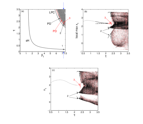
Figure 2(a) is a bifurcation diagram in $(\beta_{1},\tau)$. It shows a supercritical Hopf (sH), a limit point bifurcation of cycles (LPC) and two period doubling (PD) bifurcation curves. In this figure, the two PD curves represent the bifurcation from period-1 to period-2 for two different branches of the limit cycle. The black PD curve corresponds to the period doubling of the stable limit cycle branch emerging from the LPC curve. On the other hand, the red one is associated with the period doubling of the limit cycle branch arising from the sH curve. Figure 2(a) also shows a chaotic region represented by gray dots. That is determined by the largest Lyapunov exponent $\lambda_{1}$ of the model in Eq. (36). For this computation, we firstly obtain the time series of DDEs from the constant history function $x_{1}(t)=x_{2}(t)=0$ for $-\tau\leq t\leq 0$. Remember that we assume the two individuals to be completely indifferent to each other when they first meet. Then, the largest Lyapunov exponent of the time series is estimated with the help of TISEAN TISEAN . The result of Fig. 2(a) also shows bistable phenomena: Two limit cycles emerging from the sH and the LPC curves coexist. Moreover, a limit cycle and a chaotic attractor coexist around the period-doubling bifurcation point ‘2’ in Fig. 2(a). It shows that the red PD curve is on the chaotic region.

In Fig. 2(b), we plot the orbit diagram, i.e., the local maxima of the $x_{1}$ variable as varying $\tau$ at a fixed $\beta_{1}=7.2$. Here, the black and the red dots are obtained from $x_{1}(t)=x_{2}(t)=0$ and $x_{1}(t)=2.4,x_{2}(t)=0.2$ for $-\tau\leq t\leq 0$, respectively. The orbit diagram corresponds to the line indicated by blue arrows in Fig. 2(a). In the following bifurcation diagrams, lines indicated by blue arrows correspond to their matching orbit diagrams. The result of Fig. 2(b) shows a cascade of period-doubling bifurcations. For a clearer illustration, we plot together the orbit diagram based on Poincare section ($x_{2}=0$) at the same fixed value $\beta_{1}=7.2$. It explicitly shows a period-doubling route to chaos. However, in the following orbit diagrams, we only plot those consisting of local extrema, because they are clearer than those based on Poincare section to understand how the bifurcation occurs. Also, Fig. 2(b) and Fig. 2(c) agree well with the result that the time delay can induce a period doubling route to chaos Kitano .

It seems appropriate to comment on more PD curves. In Fig. 2(a), we could not present more PD curves corresponding to the bifurcation from period-2 to period-4 or for higher period because numerical detection and continuation of a bifurcation point in DDEs is more subtle than that of ODEs. However, the result of the orbit diagram in Fig. 2(b) clearly explains that there exists a cascade of period doubling bifurcations in Fig. 2(a). Concerning this diagram, the non-zero history function does not agree with our real experience and the assumption on initial indifference. However, we add it to clarify the bistable phenomena observed in Fig. 2(a). The orbit diagram explicitly shows two coexisting limit cycles and the coexistence of a limit cycle and a chaotic attractor. The points ‘2’ and ‘3’ in Figs. 2(a) and 2(b) represent the same points.

Figure 2: (a) Bifurcation diagram in $(\beta_{1},\tau)$ for the parameter value: $\alpha_{1}=\alpha_{2}=1$, $\beta_{2}=1$, and $\gamma_{1}A_{2}=\gamma_{2}A_{1}=0.5$. (b) Orbit diagram of local maxima of $x_{1}$ at a fixed value $\beta_{1}=7.2$. (c) Orbit diagram based on Poincare section ($x_{2}=0$).

Figure 3: Branch of the limit cycle emanating from the Hopf point and the steady state for the parameter value: $\alpha_{1}=\alpha_{2}=1$, $\beta_{1}=7.2$, $\beta_{2}=1$, and $\gamma_{1}A_{2}=\gamma_{2}A_{1}=0.5$. The points ‘1’ and ‘2’ represent the same points in Figs. 2(a) and 2(b).

Figure 4: (a,b) Time series and (c) phase plot of the model in Eq. (36) for the parameter value: $\alpha_{1}=\alpha_{2}=1$, $\beta_{1}=7.2$, $\beta_{2}=1$, $\gamma_{1}A_{2}=\gamma_{2}A_{1}=0.5$, and $\tau=3.2$. The results are obtained from $x_{1}(t)=x_{2}(t)=0$ for $t\leq 0$.

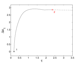
Now, let us show that the Hopf bifurcation in Fig. 2(a) is supercritical. Though, for determining the direction of Hopf bifurcation, rigorous analysis based on the normal form method and the center manifold theory presented in Refs. Wei ; Hassard is required, numerical bifurcation analysis can be used to investigate it. In Fig. 3, we obtain the variation of the amplitude $\Delta{x_{1}}=\mathrm{max}\big{(}x_{1}(t)\big{)}-\mathrm{min}\big{(}x_{1}(t)\big{)}$ for the limit cycle branch emerging from the Hopf bifurcation point ‘1’ with increasing $\tau$ at a fixed $\beta_{1}=7.2$. The solid and the dashed curves represent the stable and the unstable branches, respectively. The result shows that a smooth transition from the steady state to the limit cycle arises across the Hopf point, supporting the Hopf bifurcation being supercritical. The limit cycle branch arising from the Hopf point loses its stability at the period-doubling bifurcation point ‘2’.

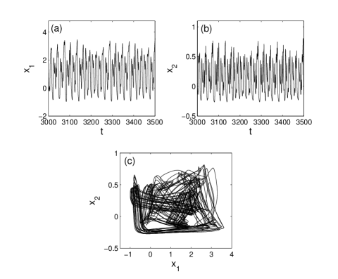
In Fig. 4, we show the time series and the phase plot of the model in Eq. (36) when it exhibits chaotic behavior ($\lambda_{1}\simeq 0.038$). The results tell us that the love dynamics of two individuals exhibits stormy patterns of feelings and a long-time unpredictable state.

Figure 5: (a) Bifurcation diagram in $(\beta_{2},\tau)$ for the parameter value: $\alpha_{1}=\alpha_{2}=1$, $\beta_{1}=1$, and $\gamma_{1}A_{2}=\gamma_{2}A_{1}=0.5$. (b) Orbit diagram of local minima of $x_{2}$ at a fixed value $\beta_{2}=7.2$.

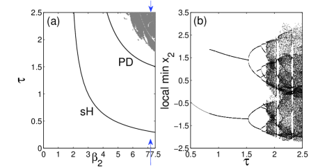
For the parameter space $(\beta_{2},\tau)$, we show the bifurcation diagram in Fig. 5(a). It consists of sH and PD curves including a chaotic region. In Fig. 5(b), we plot the orbit diagram of local minima of $x_{2}$ for fixed $\beta_{2}=7.2$. Here, the orbit diagram is obtained from $x_{1}=x_{2}=0$ for $t\leq 0$ and clearly shows a period-doubling route to chaos. The results of Figs. 5(a) and 5(b) are same as those of Figs. 2(a) and 2(b) except for the bistable phenomena. In both parameter spaces $(\beta_{1},\tau)$ and $(\beta_{2},\tau)$, we observe the same bifurcation structure consisting of a supercritical Hopf and a cascade of period-doubling bifurcations, that is, a period-doubling route to chaos.

Through a numerical bifurcation analysis, we have confirmed the theoretical predictions on the occurrence of a Hopf bifurcation and obtained the following results: For $\beta_{i}$ smaller than ${\beta_{i}}^{c}$, a steady state of love dynamics cannot be destabilized by a Hopf bifurcation, no matter how long $\tau$ is. That is, the existence of time delay does not influence a plateau of the love affair for insensitive couple. ${\beta_{i}}^{c}$ is a minimum value of $\beta_{i}$, which satisfies the inequality of Eq. (27) for given parameter values. In those cases, ${\beta_{1}}^{c}\simeq 1.27$ and ${\beta_{2}}^{c}\simeq 1.68$. For $\beta_{i}>{\beta_{i}}^{c}$, the parameter value of $\tau$, where the supercritical Hopf bifurcation arises, becomes shorter as $\beta_{i}$ increases. For large $\beta_{i}$ and long $\tau$, the limit cycle undergoes a cascade of period doubling bifurcations resulting in chaotic motion, i.e., stormy patterns of feelings.

IV.2 Synergic Couple

Let us now investigate the synergic couple. For the same reason as in the non-synergic case, the couple composed of a secure and a non-secure individuals are considered. Then, the love dynamics is given by

$$\dot{x_{1}}(t)=-\alpha_{1}x_{1}(t) + {R_{1}}^{s}\big{(}x_{2}(t-\tau)\big{)}$$

$$+ \big{\{}1+S_{1}\big{(}x_{1}(t)\big{)}\big{\}}\,\gamma_{1}A_{2},$$

$$\dot{x_{2}}(t)=-\alpha_{2}x_{2}(t) + {R_{2}}^{n}\big{(}x_{1}(t-\tau)\big{)}$$

$$+ \big{\{}1+S_{2}\big{(}x_{2}(t)\big{)}\big{\}}\,\gamma_{2}A_{1},$$

where the functional forms of the secure return ${R_{1}}^{s}$ and the non-secure return ${R_{2}}^{n}$ are described by Eqs. (6) and (10), respectively. Here, the synergic functions ${S_{1}}$ and ${S_{2}}$ are given by Eq. (12).

Figure 6: (a) Bifurcation diagram in $(\beta_{1},\tau)$ for the parameter value: $\alpha_{1}=\alpha_{2}=1$, $\beta_{2}=1$, $\gamma_{1}A_{2}=\gamma_{2}A_{1}=0.5$, and $\sigma_{1}=\sigma_{2}=0.5$. (b) Orbit diagram of local minima of $x_{2}$ at a fixed value $\beta_{1}=9.05$.

Figure 7: (a) Bifurcation diagram in $(\beta_{2},\tau)$ for the parameter value: $\alpha_{1}=\alpha_{2}=1$, $\beta_{1}=1$, $\gamma_{1}A_{2}=\gamma_{2}A_{1}=0.5$, and $\sigma_{1}=\sigma_{2}=0.5$. (b) Orbit diagram of local minima of $x_{2}$ at a fixed value $\beta_{2}=4.3$.

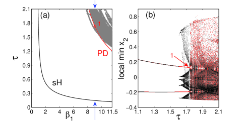
For the parameter space $(\beta_{1},\tau)$, we plot the bifurcation and the orbit diagrams of the model in Eq. (IV.2) in Figs. 6(a) and 6(b), respectively. In Fig. 6(b), the black and the red dots are obtained from $x_{1}(t)=x_{2}(t)=0$ and $x_{1}(t)=2.4,x_{2}(t)=0.2$ for $t\leq 0$, respectively. The above results exhibit bistable phenomena. The point ‘1’ in Figs. 6(a) and 6(b) represents the same point, which corresponds to a period doubling of the limit cycle branch arising from the sH curve. However, we cannot continue other bifurcation curves involved in the bistable phenomena, such as the LPC and the black PD curves in Fig. 2(a).

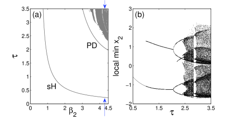
In Figs. 7(a) and 7(b), we present the results of the numerical bifurcation analysis for the parameter space $(\beta_{2},\tau)$. Here, the orbit diagram is obtained from $x_{1}(t)=x_{2}(t)=0$ for $t\leq 0$. Equivalently to the non-synergic case, the results of Figs. 7(a) and 7(b) are the same as those for Figs. 6(a) and 6(b) except for the bistable phenomena. Therefore, we explicitly show that a supercritical Hopf and a cascade of period-doubling bifurcations, i.e., a period-doubling route to chaos, is a universal bifurcation structure in our models in Eqs. (36) and (IV.2). For the synergic case, we identify that ${\beta_{1}}^{c}\simeq 0.79$ and ${\beta_{2}}^{c}\simeq 0.60$.

V Conclusion

In conclusion, we have investigated the effect of time delay on a simplified mathematical model that describes the dynamics of love between two individuals in the field of social science. By analyzing the characteristic equation of linearization of the model, we have theoretically proven that if no one exhibits a non-secure return in both cases of synergic and non-synergic couples, then the existence of time delay cannot disturb a steady state of love dynamics. However, if at least one of them has a non-secure return, then the time delay on the return function can cause a Hopf bifurcation and a cyclic love dynamics. Through a numerical bifurcation analysis, we have confirmed the theoretical predictions on the occurrence of the Hopf bifurcation and obtained the universal bifurcation structure consisting of a supercritical Hopf and a cascade of period-doubling bifurcations, resulting in chaotic motion, which exhibits stormy patterns of feelings and a long-time unpredictable state. We have also ascertained that the existence of time delay does not influence a steady state of the love affair for an insensitive couple.

Through further investigation, we hope that the time delay effect on a more realistic love dynamical model, including a love triangle, can be investigated. Moreover, it seems that such modeling approach with time delay can be applied to various dynamical phenomena in the field of social science, including a study of the proper relation between supplier and consumer in the field of management.