Phase transition in the Jarzynski estimator
of free energy differences

Abstract

The transition between a regime in which thermodynamic relations apply only to ensembles of small systems coupled to a large environment and a regime in which they can be used to characterize individual macroscopic systems is analyzed in terms of the change in behavior of the Jarzynski estimator of equilibrium free energy differences from nonequilibrium work measurements. Given a fixed number of measurements, the Jarzynski estimator is unbiased for sufficiently small systems. In these systems the directionality of time is poorly defined and the configurations that dominate the empirical average, but which are in fact typical of the reverse process, are sufficiently well sampled. As the system size increases the arrow of time becomes better defined. The dominant atypical fluctuations become rare and eventually cannot be sampled with the limited resources that are available. Asymptotically, only typical work values are measured. The Jarzynski estimator becomes maximally biased and approaches the exponential of minus the average work, which is the result that is expected from standard macroscopic thermodynamics. In the proper scaling limit, this regime change has been recently described in terms of a phase transition in variants of the random energy model (REM). In this paper, this correspondence is further demonstrated in two examples of physical interest: the sudden compression of an ideal gas and adiabatic quasi-static volume changes in a dilute real gas.

I Introduction

The laws of thermodynamics summarize empirical observations about the approximate and most probable behavior of macroscopic systems Gibbs (1902); Khinchin (1949); Zwanzig (2001); Castiglione et al. (2008). They are formulated under the assumption of limited resources in the measurements of the quantities involved. In the words of Gibbs, thermodynamics laws “express the laws of mechanics for [systems of a great number of particles] as they appear to beings who have not the fineness of perception to enable them to appreciate quantities of the order of magnitude of those which relate to single particles, and who cannot repeat their experiments often enough to obtain any but the most probable results” Gibbs (1902). This statement summarizes the conditions under which a proper thermodynamic description for a single system can be made: (i) the system has a large number of degrees of freedom, (ii) the quantities of interest involve averages over space and time on scales that are large compared to the corresponding molecular scales, (iii) there are limitations in the time span of the measurements, and (iv) there are limitations in the number of measurements made. For instance, the elimination of condition (iii) gives rise to the objection formulated by Zermelo, based on the fact that any isolated mechanical system will come arbitrarily close to its initial state provided that a sufficiently long period of time elapses (Poincaré recurrences)Zermelo (1896); Zwanzig (2001); Castiglione et al. (2008). If the system is ergodic, averages over phase-space can be replaced by time averages and conditions (iii) and (iv) are equivalent.

Improvements in measurement devices and techniques, an increasing interest in smaller scale systems in biology, physics and chemistry Liphardt et al. (2002); Barkai et al. (2004); Bustamante et al. (2005); Ruschhaupt et al. (2006); Thorn et al. (2008); Ritort (2008) and developments in dynamical systems and chaos theory Gaspard (1998) have prompted numerous researchers to develop interpretations and extensions of thermodynamics applicable to systems with small numbers of degrees of freedom Oppenheim and Mazur (1957); Mazur and Oppenheim (1957); Lebowitz and Percus (1961); Hill (1963); Bustamante et al. (2005); Seifert (2008). In such systems it is not possible to uphold the standard interpretation of the thermodynamic quantities and of their relations. In particular, the measurements are made on molecular scales and produce values that are dominated by fluctuations. Nonetheless, reproducible results are obtained by performing averages over many independent measurements of small systems at equilibrium (e.g., in contact with a heat bath). Therefore, a proper thermodynamic description is recovered if the ensemble method, which was originally devised as an operational construct to obtain results for single macroscopic systems, is given a literal interpretation: Thermodynamic quantities are identified with ensemble averages, which are experimentally realized as averages over independent measurements under equilibrium conditions. Note that the condition of equilibrium requires that the small system be in contact with some other system with a large number of degrees of freedom (e.g. a heat reservoir for the canonical ensemble), so that correct results are obtained from the assumption that the initial state in a particular realization of the process can be treated as an independent sample from the appropriate ensemble. Thus, conditions (i)-(iv) are required for the whole and are essential for a proper thermodynamic description of the small system as well.

In this work we investigate the transition between the regime in which the thermodynamic description is valid for a single system and the regime in which thermodynamic quantities need to be understood as averages over realizations of a given process. To this end we analyze the behavior of the empirical estimates of equilibrium free energy differences from nonequilibrium work measurements by means of the Jarzynski equality. In contrast to standard thermodynamic relations, the ensemble average that appears in the Jarzynski equality is dominated by rare extreme fluctuations Jarzynski (2006). Consequently, to obtain accurate estimations of the free energy change, one needs to perform repeated work measurements in the nonequilibrium process. The number of measurements needed to obtain meaningful estimates increases exponentially with the size of the system Gore et al. (2003); Jarzynski (2006). Therefore, the average that appears in the Jarzynski equality cannot be realized in the macroscopic regime, in which definite values of thermodynamic quantities can be ascribed to single systems rather than to collections of systems.

For limited resources, when the number of measurements is fixed, the Jarzynski estimator of free energy differences becomes biased as the size of the system increases. In the appropriate scaling limit, the appearance of the bias is abrupt and corresponds to a phase transition in variants of the random energy model (REM) Derrida (1980, 1981); Moukarzel and Parga (1991); Bovier et al. (2002); Ogure and Kabashima (2009). The connection between the random energy model and the Jarzynski estimator of free energy differences was made in Palassini and Ritort (2008a, b, 2011). In those articles, expressions of the free energy in the low-temperature (small $M$ limit, where $M$ is the number of nonequilibrium work measurements) and in the high-temperature phases (large $M$ limit) of the random energy model, including finite $M$ corrections, were derived for a parametric family of work distributions. In another recent work, the convergence of Monte Carlo estimates in terms of the random energy model has been made in connection with the ’sign problem’ Düring and Kurchan (2010).

In the current paper we further establish the correspondence between the Jarzynski estimator of free energy differences and variants of the random energy model for the sudden compression of an ideal gas and for adiabatic quasi-static volume changes in a dilute real gas. Even though this correspondence is explicitly established for only a few particular physical systems, it is expected to obtain in more general situations. The origin of the phase transitions in sums of random exponentials is the interplay between classic limit theorems for sums (e.g., the central limit theorem, the law of large numbers) and extreme value statistics Ben Arous et al. (2005); Clusel and Bertin (2008). A contribution of this paper is to highlight the importance of the phase transition in the Jarzynski estimator of free energy differences to signal the change between two distinct regimes wherein the ensemble and the single-system interpretations of thermodynamic quantities are applicable, respectively.

The article is organized as follows: Section II introduces the Jarzynski equality and related concepts that are necessary for the subsequent study. The use of this equality in the estimation of equilibrium free energy differences from nonequilibrium work values is described in Section III. Section IV analyzes the change in behavior of the Jarzynski estimator as a function of system size and of the number of measurements performed in three illustrative examples. Finally, Section V discusses how this change in behavior corresponds to the emergence of classical macroscopic thermodynamics and a well-defined arrow of time as the size of the system is increased, when the number of measurements performed is fixed. The technical details of the analysis of the Jarzynski estimator in terms of variants of the random energy model are deferred to the appendices.

II The Jarzynski equality

Consider a system characterized by a Hamiltonian $H(\Gamma;\lambda)$, where $\Gamma$ denotes a point in phase space. The parameter $\lambda$ can be modified by external manipulation to perform or extract work from the system. If the system is coupled to other degrees of freedom, the changes in $\lambda$ are assumed to affect only the Hamiltonian of the system of interest and not the terms that describe its interaction with the environment or the environment itself.

Assume that the parameter $\lambda$ is modified in the interval $[0,\tau]$ according to a specified protocol $\left\{\lambda(t);\,0\leq t\leq\tau\right\}$ from $\lambda(0)=\lambda_{0}$ to $\lambda(\tau)=\lambda_{1}$. It is possible to show that the work associated with the transition between an initial configuration of the system sampled from an equilibrium distribution with Hamiltonian $H_{0}(\Gamma)\equiv H(\Gamma;\lambda_{0})$ at temperature $\beta^{-1}$ and a final configuration corresponding to the Hamiltonian $H_{1}(\Gamma)\equiv H(\Gamma;\lambda_{1})$ is a random variable $W$ that satisfies the equality Jarzynski (1997, 2004)

$$\left<e^{-\beta W}\right>=e^{-\beta\Delta F},\quad\Delta F=F_{1}-F_{0}.$$ (1)

The average is performed over trajectories whose initial point in phase space is sampled from a canonical distribution

$$\frac{e^{-\beta H_{0}(\Gamma)}}{\int_{\Omega}d\Gamma e^{-\beta H_{0}(\Gamma)}},$$ (2)

where the integral is over $\Omega$, the region of phase space accessible to the system. This region is assumed to remain unchanged during the process. Note that the state in which the system finds itself after the manipulation has been completed need not be an equilibrium one. In general, $F_{1}$ is not the free energy of such a state. Therefore, the free energy difference that appears on the right-hand side of (1)

$$F_{i}=-\beta^{-1}\log\int_{\Omega}d\Gamma e^{-\beta H_{i}(\Gamma)},\quad i=0,1,$$ (3)

need not coincide with the actual free energy change in the process described Jarzynski (2004); Palmieri and Ronis (2007). It is the difference between the free-energies of the system in equilibrium at temperature $\beta^{-1}$ in two states characterized by Hamiltonians $H_{0}$ and $H_{1}$, respectively. If the system is strongly coupled with an environment that acts as a heat reservoir, $H(\Gamma;\lambda)$ is the potential of mean force associated with the variables of the system of interest Kirkwood (1935); Jarzynski (2004). If the system is isolated or weakly coupled with its environment during the external manipulation, $H(\Gamma;\lambda)$ can be identified with the Hamiltonian of the isolated system Jarzynski (1997).

III Estimation of free energy differences from nonequilibrium work measurements

Since it was derived the Jarzynski equality has attracted a fair amount of interest because it allows the computation of equilibrium free energy differences from measurements of work in general nonequilibrium processes

$$\Delta F=-\beta^{-1}\log\left<e^{-\beta W}\right>,$$ (4)

where the angular brackets denote an average over the canonical ensemble at temperature $\beta^{-1}$ with respect to the initial Hamiltoninan $H_{0}$. However, this equality differs in crucial aspects from standard thermodynamic relations. Because of the molecular nature of the systems analyzed, thermodynamic quantities (energy density, number density, temperature, pressure, work, etc.) are fluctuating variables. In macroscopic systems, the fluctuations are small. This allows us to identify these random thermodynamic quantities with their typical values, which are deterministic and can be measured in single experiments. Repetitions of these experiments yield values that are indistinguishable, within the error of the macroscopic measurement. Therefore, for standard thermodynamic quantities, typical and average values are close to each other and can be used interchangeably to characterize the macroscopic state of the system under study.

In contrast, the average that appears in the Jarzynski equality needs to be interpreted as a true ensemble average Jarzynski (1997). The work measured in a particular realization of a nonequilibrium process depends on the initial microscopic configuration of the system and is therefore a fluctuating quantity. In each of these measurements, the system is prepared in an initial state sampled from the equilibrium distribution. One then carries out the intervention that gives rise to the nonequilibrium process. The work involved in this process is then recorded. Finally, to extract equilibrium free energy differences from these measurements, the average of the exponential of minus these work values is computed. Because of the exponential form of the summed quantities, typical and average values are, in the general case, very different. Unlike for standard thermodynamic relations, plugging in the typical value of the work on the left-hand side of (1) does not fulfill the equality. The reason is that the average is dominated by extreme events whose probability of occurrence is very low. Therefore, a sufficiently large number of measurements is needed so that these rare events are well represented and the equality can be empirically realized. The number of measurements required to provide a meaningful estimate of the average increases exponentially with the size of the system Gore et al. (2003); Lua and Grosberg (2005); Jarzynski (2006). Therefore, it is not practicable in macroscopic systems. Nonetheless, the regime in which the equality can be experimentally verified is accessible for sufficiently small systems.

To realize the average, repeated experiments under the same conditions are carried out. The values of work obtained in each of these experiments are recorded and used to estimate the average

$$\left<e^{-\beta W}\right>\approx\left<e^{-\beta W}\right>_{M}\equiv\frac{1}{M}\sum_{m=1}^{M}e^{-\beta W_{m}}.$$ (5)

By means of the Jarzynski equality, this Monte Carlo average can be used to estimate the change in free energy

$$\Delta F_{M}\equiv-\beta^{-1}\log\left<e^{-\beta W}\right>_{M}.$$ (6)

Since the particular realization of work values $\left\{W_{m}\right\}_{m=1}^{M}$ is random, the estimate $\Delta F_{M}$ is also a random variable. Our goal is to understand the properties of this random variable as a function of $M$, the number of nonequilibrium work measurements and $N$, the size of the system.

Because of the exponential form of the quantity averaged, the role of extreme fluctuations is very important. In contrast to usual thermodynamic averages, such as $\left<W\right>$, the average work, which are dominated by configurations that are typical of the initial (equilibrium) state of the system, the average $\left<e^{-\beta W}\right>$ is actually dominated by rare configurations that are typical of the system at equilibrium at temperature $\beta^{-1}$ with respect to the final Hamiltonian Jarzynski (2006).

Of particular interest is the block Zuckerman and Woolf (2002, 2004) or quenched Mézard and Montanari (2009) average

$$\mathbb{E}\left[\Delta F_{M}\right]\equiv-\beta^{-1}\mathbb{E}\left[\log\left<e^{-\beta W}\right>_{M}\right],$$ (7)

where the expectation $\mathbb{E}\left[\cdot\right]$ is with respect to independent realizations of $M$ measurements, each of which corresponds to an independent sample from an initial equilibrium canonical distribution at temperature $\beta^{-1}$. In Zuckerman and Woolf (2002, 2004) $\mathbb{E}\left[\Delta F_{M}\right]$ is referred to as the finite-data average free energy. This quantity is an estimator of $\Delta F$, albeit a biased one, in general. The bias is the difference between the expected value of this estimator and the actual value of the free energy

$$B_{M}\equiv\mathbb{E}\left[\Delta F_{M}\right]-\Delta F.$$ (8)

Using the law of large numbers it is possible to show that in the limit $M\rightarrow\infty$ the block average converges to the free energy change

$$\lim_{M\rightarrow\infty}\mathbb{E}\left[\Delta F_{M}\right]=\Delta F.$$ (9)

Therefore, the estimator $\mathbb{E}\left[\Delta F_{M}\right]$ is asymptotically unbiased

$$\lim_{M\rightarrow\infty}B_{M}=0.$$ (10)

For a single experiment $M=1$ the estimator equals the average work performed on the system

$$\mathbb{E}\left[\Delta F_{1}\right]=\left<W\right>.$$ (11)

Following Gore et al. (2003), we define the ‘dissipated work’ in a given realization of the experiment as

$$W_{dis}=W-\Delta F.$$ (12)

Using Jensen’s inequality it is possible to show that $\mathbb{E}\left[\Delta F_{1}\right]$ is a positively biased estimator of $\Delta F$

$$\left<W\right>=\mathbb{E}\left[\Delta F_{1}\right]\geq\Delta F.$$ (13)

In fact, the convergence of $\mathbb{E}\left[\Delta F_{M}\right]$ to the asymptotic limit $\Delta F$ is monotonic Zuckerman and Woolf (2004)

$$\left<W\right>=\mathbb{E}\left[\Delta F_{1}\right]\geq\mathbb{E}\left[\Delta F_{M}\right]\geq\mathbb{E}\left[\Delta F_{M+1}\right]\geq\mathbb{E}\left[\Delta F_{\infty}\right]=\Delta F,\quad 1<M<\infty.$$ (14)

In terms of the bias

$$\left<W_{dis}\right>=\left<W\right>-\Delta F=B_{1}\geq B_{M}\geq B_{M+1}\geq B_{\infty}=0,\quad 1<M<\infty.$$ (15)

Therefore, the maximum bias corresponds to $M=1$ and coincides with the average dissipated work

$$B_{\max}=B_{1}=\left<W_{dis}\right>.$$ (16)

The main contribution of this research is to explicitly show in several paradigmatic cases that the finite sample estimate of free energy differences from the Jarzynski equality for a particular system exhibits a change of behavior as $M$, the number of repetitions of the experiment, increases. Alternatively, for a fixed number of measurements, the regime change occurs as a function of $N$, the system size. For small systems the Jarzynski estimator is unbiased. In these systems the nonequilibrium work measurements are dominated by fluctuations. Configurations that are typical of the reversed process are well sampled, which means that the arrow of time is poorly defined. As the system size increases, the probability of sampling these configurations becomes exponentially small, so that they are not observed in practice. The Jarzynski estimator of the free energy change becomes biased and asymptotically approaches the value of the average work. The suppression of these fluctuations also leads to the emergence of a well-defined arrow of time in the system. In the limit $M\rightarrow\infty$, $N\rightarrow\infty$ with $\log M/N\rightarrow\text{constant}$ the regime change is akin to a phase transition that arises in simplified models of spin-glasses, such as the random energy model in both its continuous Derrida (1980, 1981) and discrete Moukarzel and Parga (1991, 1992); Ogure and Kabashima (2009) versions.

IV Phase transition in the Jarzynski estimator of free energy differences

We now proceed to analyze the behavior of the Jarzynski estimator in three important cases. The first one corresponds to processes in which the nonequilibrium work distribution is Gaussian Gore et al. (2003). This is a particular case of the class of work distributions analyzed in Palassini and Ritort (2011) with $\delta=2$. The second case is a compression experiment for an ideal gas Lua and Grosberg (2005); Presse and Silbey (2006); Palmieri and Ronis (2007). Finally, we consider adiabatic and quasi-static volume changes for a dilute classical gas of interacting particles Crooks and Jarzynski (2007).

The change of regime is best analyzed in terms of the normalized bias

$$\tilde{B}_{M}\equiv\frac{B_{M}}{B_{\max}}=\frac{\mathbb{E}\left[\Delta F_{M}\right]-\Delta F}{\left<W\right>-\Delta F},\quad 0\leq\tilde{B}_{M}\leq 1,$$ (17)

where the maximum bias is the difference between the average work in the actual nonequilibrium process (which is not necessarily isothermal) and the free energy difference in the corresponding isothermal process

$$B_{\max}=\left<W\right>-\Delta F.$$ (18)

As a function of $M$, the normalized bias is a monotonically decreasing quantity of $M$, which is bounded between $0$ and $1$

$$1=\tilde{B}_{1}\geq\tilde{B}_{M}\geq\tilde{B}_{M+1}\geq\tilde{B}_{\infty}=0,\quad 1<M<\infty.$$ (19)

To simplify the derivations we assume $\beta=1$. It is straightforward to reintroduce this parameter in the final expressions by noting that setting $\beta=1$ is equivalent to measuring energies in units of $\beta^{-1}=k_{B}T$, where $k_{B}$ is the Boltzmann constant and $T$ is the initial equilibrium temperature.

IV.1 Gaussian work distribution

In this section, we illustrate the connection between the Jarzynski free energy difference estimator and the random energy model for a Gaussian work distribution. The results presented in this section were first derived in Palassini and Ritort (2011). That reference gives explicit expressions for the bias of the Jarzynski estimator in different regimes for a general class of work distributions, which includes the Gaussian as a particular case. It also considers finite-size corrections, which are ignored in our analysis.

Assume that in the sample estimate

$$\left<e^{-W}\right>_{M}=\frac{1}{M}\sum_{m=1}^{M}e^{-W_{m}}.$$ (20)

the work values $\left\{W_{m}\right\}_{m=1}^{M}$ follow a normal distribution whose mean is $<W>$, and whose variance is $\sigma^{2}$ Gore et al. (2003). In this case,

$$\Delta F=-\log\left<e^{-W}\right>=\left<W\right>-\frac{1}{2}\sigma^{2}.$$ (21)

Therefore, the maximum bias is

$$B_{\max}=\left<W\right>-\Delta F=\frac{1}{2}\sigma^{2}.$$ (22)

This is an extensive quantity and scales with the size of the system. In the limit $\sigma\rightarrow\infty$, $M\rightarrow\infty$ and $\log M/\sigma^{2}$ finite, the estimate of the free energy has an abrupt change of behavior (see appendix A)

$$\mathbb{E}\left[\Delta F_{M}\right]=\left\{\begin{array}[]{ll}\left<W\right>-\frac{1}{2}\sigma^{2},&M\geq\exp\left\{\frac{1}{2}\sigma^{2}\right\}\\ \left<W\right>-\sqrt{2}\sigma\sqrt{\log{M}}+\log M,&M<\exp\left\{\frac{1}{2}\sigma^{2}\right\}.\end{array}\right.$$ (23)

These expressions correspond to those derived in Palassini and Ritort (2011) (Eq. (4) and the paragraph before this equation in that reference) for $\delta=2,$ $\Omega^{2}=2\sigma^{2},$ $N=M$, and $D_{c}=\sigma^{2}/2$.

For a fixed value of $\sigma$ the normalized bias is

$$\tilde{B}_{M}=\frac{B_{M}}{B_{\max}}=\left\{\begin{array}[]{ll}0,&M\geq M_{c}\\ \left(1-\sqrt{\log M/\log M_{c}}\right)^{2},&M<M_{c}\end{array}\right.$$ (24)

with $M_{c}=\exp\left\{\frac{1}{2}\sigma^{2}\right\}$.

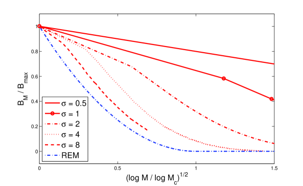
Figure 1 displays the dependence of the normalized bias (24) as a function of $\sqrt{\log M/\log M_{c}}$ with a fixed $\sigma$, for different values of $\sigma$. The curve corresponding to the asymptotic limit $\sigma\rightarrow\infty$ is plotted as a dash-dotted line. The remaining curves are averages over Monte Carlo simulations. For small numbers of measurements ($M<M_{c}$), the Jarzynski estimator is biased. In this regime, the free energy exhibits strong (of order 1) non-Gaussian fluctuations around its average (Theorem 1.6 from Bovier et al. (2002)). These fluctuations are driven by the Poisson process of the extremes of the random nonequilibrium work measurements. The range $M>M_{c}$ corresponds to a regime in which the estimate of the free energy change for sufficiently large $\sigma$ is unbiased. The bias persists beyond this limit for small systems: when $\sigma$ is small, the transition between regimes is more gradual. This is the region in which one expects to observe convergence to the Jarzynski limit in experiments. There is a second phase transition in the system: in the range $e^{\sigma^{2}/2}<M<e^{\sigma^{2}}$ the fluctuations can be expressed in terms of the Poisson process of extremes of the nonequilibrium work measurements. Beyond the threshold $M_{c}^{{}^{\prime}}=e^{\sigma^{2}}$, the central limit theorem holds and the fluctuations around the block average are approximately Gaussian (Theorem 1.5 from Bovier et al. (2002)). The graph presented corresponds to Fig. 2(a) in Palassini and Ritort (2011), with $\sigma^{2}=\Omega^{2}/2$. The main difference is the square root in the abscissae, which does not modify the point at which the phase transition occurs in the REM limit or the qualitative picture.

Table 1 displays the number of measurements needed to obtain an unbiased estimate of the free energy using the Jarzynski estimator ($M_{c}$) and to reach a regime in which the fluctuations around this estimate are Gaussian ($M_{c}^{{}^{\prime}}$) for the several values of $B_{max}$ in the range explored in the experiments described in Palassini and Ritort (2011) (from $k_{B}T$ to $20k_{B}T$).

Table 1: Number of measurements needed to obtain an unbiased estimate of the free energy ($M_{c}$) and to reach a regime in which the fluctuations around this estimate are Gaussian ($M_{c}^{{}^{\prime}}$) as a function of $B_{max}$, when the nonequilibrium work distribution is Gaussian.

$B_{max}$	$k_{B}T$	$2k_{B}T$	$5k_{B}T$	$10k_{B}T$	$20k_{B}T$
$M_{c}$	3	8	149	22,027	485,165,196
$M_{c}^{{}^{\prime}}$	8	55	22,027	485,165,196	$2.35\cdot 10^{17}$

Figure 1: Approach of the normalized bias to the curve (24) as $M\rightarrow\infty$. The random energy model corresponds to the dash-dotted line.

The regime change can also be observed when the number of measurements is fixed and the size of the system, measured in terms of $\sigma^{2}$, increases. For a fixed $M$, the normalized bias is

$$\tilde{B}_{M}=\frac{B_{M}}{B_{\max}}=\left\{\begin{array}[]{ll}0,&\sigma\leq\sigma_{c}\\ \left(1-\sigma_{c}/\sigma\right)^{2},&\sigma>\sigma_{c}\end{array}\right.,$$ (25)

where $\sigma_{c}=\sqrt{2\log M}$.

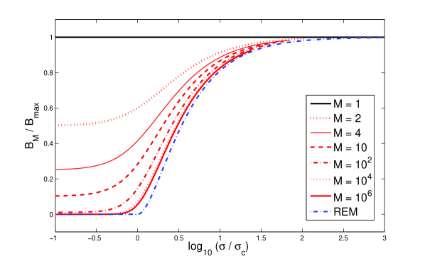
Figure 2 displays the curves that trace the dependence of the normalized bias (25) as a function of $\log_{10}(\sigma/\sigma_{c})$ with $M$ fixed, for different values of $M$. The curve corresponding to the random energy model ($M\rightarrow\infty$) is displayed as a dash-dotted line. In small systems $\sigma<\sigma_{c}$ the estimate of the free energy difference is unbiased. For sufficiently small systems ($\sigma\rightarrow 0$), the bias scales as $B_{M}\sim B_{\max}/M$. Therefore, the bias is reduced by increasing $M$ linearly. This is the region in which one expects convergence of the sample average to the Jarzynski equality limit. Beyond that threshold ($\sigma>\sigma_{c}$), the empirical estimate is biased. As the system size increases the bias approaches its maximum value, which corresponds to measuring the typical value in most of the nonequilibrium work measurements, in agreement with the expected behavior of classical macroscopic systems. In this regime, linear increases in $M$ do not lead to significant changes in the bias observed.

Figure 2: Approach of the normalized bias to the curve (25) as $M\rightarrow\infty$. The random energy model corresponds to the dash-dotted curve.

IV.2 Ideal gas compression experiment

Consider an isolated system consisting of $N$ non-interacting particles (ideal gas). The system is confined in the interval $[-L,L]$ in the X direction. The macroscopic state of the system is defined by the temperature and the value of an externally applied potential. The microscopic state of the system is characterized by $n$, the number of particles in region II ($0<x\leq L$). Correspondingly, the number of number of particles in region I ($-L\leq x\leq 0$) is $N-n$.

Initially, the external potential is zero and the system is assumed to be in a homogeneous equilibrium state at temperature $\beta^{-1}=1$. The probability of having $n$ particles in region II in this state is

$$p(n;0) = \frac{1}{2^{N}}\binom{N}{n},\quad n=0,1,\ldots,N.$$ (26)

This is a binomial distribution with the parameters $(N,1/2)$. It is peaked around the mean $n^{*}(0)=N/2$. Its standard deviation is $\sqrt{N}/2$. The corresponding free energy is

$$F_{N}(0)=-\log\left(\frac{1}{2^{N}}\sum_{n=0}^{N}\binom{N}{n}\right)=0.$$ (27)

Consider a compression experiment during which the system undergoes a sudden transition from the initial homogeneous equilibrium state to a state in which particles are more likely to be in region I because of the presence of a positive external potential in region II

$$V(x;\epsilon)=\left\{\begin{array}[]{lrlll}0,&-L&\leq&x\leq 0\quad\hbox{[region I]}\\ \epsilon,&0&<&x\leq L\quad\hbox{[region II]}\end{array}\right..$$ (28)

The equilibrium distribution at temperature $\beta^{-1}=1$, when the system is subject to this external potential is a binomial distribution with parameters $\left(N,e^{-\epsilon}/(1+e^{-\epsilon})\right)$

$$p(n;\epsilon) = \frac{1}{\left(1+e^{-\epsilon}\right)^{N}}\binom{N}{n}e^{-n\epsilon},\quad n=0,1,\ldots,N.$$ (29)

This distribution is peaked around its mean $n^{*}(\epsilon)=N/(1+e^{\epsilon})$. Its standard deviation is $\sqrt{N}e^{-\epsilon/2}/\left(1+e^{-\epsilon}\right)$. The corresponding free energy is

$$F_{N}(\epsilon)=-\log\left[\frac{1}{2^{N}}\sum_{n=0}^{N}\binom{N}{n}e^{-n\epsilon}\right]=N\log\frac{2}{1+e^{-\epsilon}}.$$ (30)

The change in free energy between the initial state, in which the system is in equilibrium at temperature $\beta^{-1}=1$, in the absence of a external potential, and an equilibrium state at the same temperature with potential $V(x;\epsilon)$ is

$$\Delta F=F_{N}(\epsilon)-F_{N}(0)=N\log\frac{2}{1+e^{-\epsilon}}.$$ (31)

As noted by several authors, this is not the change of free energy between the equilibrium states corresponding to the initial and final values of the work parameter in the experiment that is being performed Jarzynski (2004); Palmieri and Ronis (2007). In particular, the configuration of the particles in the system at $t=0^{+}$ is the same as in the initial state because there has not been any time to evolve. In most cases, this configuration is very atypical of the equilibrium state for the new constraints. In fact, the system does not have a well-defined temperature in this state. Nonetheless, using the equality

$$\Delta F=-\log\left<e^{-W}\right>,$$ (32)

it is possible to compute the change in free energy in an isothermal process (31) in terms of the external work performed on the system during the compression Presse and Silbey (2006).

In practice, one needs to carry out a series of independent realizations of the experiment. In the $m$th realization, the configuration of the system is sampled from the equilibrium distribution $n_{m}\sim p(n;0)$. The external work needed to perform the transition in this particular realization is $W_{m}=n_{m}\epsilon$. The average work over $M$ realizations of the experiment is

$$\left<W\right>_{M}=\frac{1}{M}\sum_{m=1}^{M}W_{m}=\frac{1}{M}\sum_{m=1}^{M}n_{m}\epsilon.$$ (33)

Since the $\left\{n_{m}\right\}_{m=1}^{M}$ are independent identically distributed random variables (iidrvs), $\left<W\right>_{M}$ is also a random variable whose average is the thermodynamic work

$$\left<W\right>=\mathbb{E}\left[\left<W\right>_{M}\right]=\frac{1}{M}\sum_{m=1}^{M}\mathbb{E}\left[n_{m}\right]\epsilon=\mathbb{E}\left[n\right]\epsilon=\frac{1}{2}N\epsilon.$$ (34)

The average and the typical value of the work performed coincide.

Consider now the Jarzynski estimator of the free-energy difference

$$\Delta F_{M}=-\log\left<e^{-W}\right>_{M}=-\log\left(\frac{1}{M}\sum_{m=1}^{M}e^{-W_{m}}\right)=-\log\left(\frac{1}{M}\sum_{m=1}^{M}e^{-n_{m}\epsilon}\right).$$ (35)

This is also a random variable whose average is

$$\mathbb{E}\left[\Delta F_{M}\right]=-\mathbb{E}\left[\log\left<e^{-W}\right>_{M}\right]=-\mathbb{E}\left[\log\left(\frac{1}{M}\sum_{m=1}^{M}e^{-W_{m}}\right)\right]=-\mathbb{E}\left[\log\left(\frac{1}{M}\sum_{m=1}^{M}e^{-n_{m}\epsilon}\right)\right].$$ (36)

For $M=1$ this average coincides with the average work

$$\mathbb{E}\left[\Delta F_{1}\right]=\left<W\right>=\frac{1}{2}N\epsilon.$$ (37)

In the limit $M\rightarrow\infty$, it converges to the free energy change

$$\lim_{M\rightarrow\infty}\mathbb{E}\left[\Delta F_{M}\right]=\Delta F=N\log\frac{2}{1+e^{-\epsilon}}.$$ (38)

There is no closed-form expression for this average for other values of $M$. However, taking advantage of the correspondence between the ideal gas compression experiment and the discrete random energy model (see appendix C), it is possible to show that there is a continuous but abrupt change in the block average

$$\mathbb{E}\left[\Delta F_{M}\right]=\left\{\begin{array}[]{ll}N\log\frac{2}{1+e^{-\epsilon}},&\epsilon\leq\epsilon_{c}(\gamma)\\ N\left[\gamma\log 2+\frac{\epsilon}{2}\left(1-\tanh\frac{\epsilon_{c}}{2}\right)\right]=N\left[\gamma\log 2+\frac{\epsilon}{1+e^{\epsilon_{c}}}\right],&\epsilon>\epsilon_{c}(\gamma)\end{array}\right.$$ (39)

in the limit $M\rightarrow\infty$, $N\rightarrow\infty$, with

$$\gamma = \frac{\log M}{N\log 2}\rightarrow\hbox{constant},$$ (40)

$$\epsilon_{c}(\gamma) = \left\{\begin{array}[]{ll}\infty,&\gamma\geq 1\\ \log\left[1-h_{2}^{-1}(1-\gamma)\right]-\log\left[h_{2}^{-1}(1-\gamma)\right],&\gamma<1\end{array}\right..$$ (43)

The function $h_{2}^{-1}(y)\in[0,1/2]$ is the inverse of the binary entropy

$$h_{2}(x)=-x\log_{2}x-(1-x)\log_{2}(1-x).$$ (44)

In this limit the bias of $\mathbb{E}\left[\Delta F_{M}\right]$ as an estimator of $\Delta F$ is

$$B_{M}=\mathbb{E}\left[\Delta F_{M}\right]-\Delta F=\left\{\begin{array}[]{ll}0,&\epsilon\leq\epsilon_{c}(\gamma)\\ N\left[\gamma\log 2+\frac{\epsilon}{2}\left(1-\tanh\frac{\epsilon_{c}}{2}\right)-\log\frac{2}{1+e^{-\epsilon}}\right],&\epsilon>\epsilon_{c}(\gamma)\end{array}\right..$$ (45)

For a fixed value of $\epsilon$ the bias is maximum for $M=1$ ($\gamma=0$, $\epsilon_{c}=0$)

$$B_{\max}(\epsilon)=B_{1}=N\left[\frac{\epsilon}{2}-\log\frac{2}{1+e^{-\epsilon}}\right]=N\log\cosh\frac{\epsilon}{2}.$$ (46)

The normalized bias is

$$\tilde{B}(\gamma,\epsilon)=\frac{B_{M}}{B_{\max}(\epsilon)}=\left\{\begin{array}[]{ll}0,&\gamma\geq\gamma_{c}(\epsilon)\\ 1-\frac{\frac{\epsilon}{2}\tanh\frac{\epsilon_{c}}{2}-\gamma\log 2}{\log\cosh\frac{\epsilon}{2}}=1-\frac{\epsilon-\epsilon_{c}}{2}\frac{\tanh\frac{\epsilon_{c}}{2}}{\log\cosh\frac{\epsilon}{2}}-\frac{\log\cosh\frac{\epsilon_{c}}{2}}{\log\cosh\frac{\epsilon}{2}},&\gamma<\gamma_{c}(\epsilon)\end{array}\right.,$$ (47)

where

$$\gamma_{c}(\epsilon)=\epsilon_{c}^{-1}(\epsilon)=1-h_{2}\left(\frac{1}{1+e^{\epsilon}}\right),$$ (48)

with $\gamma_{c}(0)=0$ and $\lim_{\epsilon\rightarrow\infty}\gamma_{c}(\epsilon)=1$.

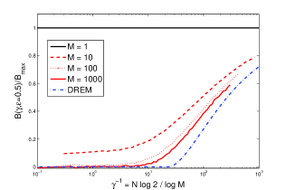
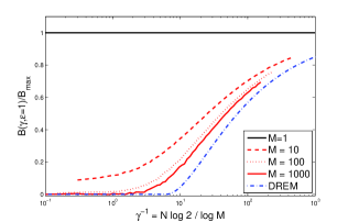
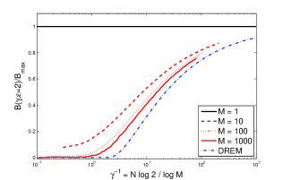
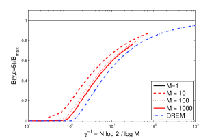
The results of computer simulations of the ideal gas compression experiment at temperature $\beta^{-1}=1$ are depicted in figure 3. The graphs display, for different values of $\epsilon$, the dependence of the normalized bias as a function of system size, measured in terms of $\gamma^{-1}$ with $M$ fixed, for different values of $M$. The behavior observed is similar to the Gaussian case: the regime in which the Jarzynski equality can be realized (i.e. the Jarzynski free energy estimator is unbiased) corresponds to gases composed of a small number of particles. If the system size is increased, assuming that the number of measurements is kept fixed, a gradual change takes place to a regime in which the Jarzynski estimator becomes biased. Asymptotically, for large $N$, the estimator becomes maximally biased, which means that only typical work values are observed. Linear increases in $M$ do not significantly reduce this bias. Therefore, in this regime, it is not possible to empirically realize the Jarzynski equality and measurements yield standard macroscopic thermodynamic values. The change in regime becomes more abrupt as $\epsilon$, $M$ and $N$ increase and is asymptotically well described by the phase transition that takes place in the discrete random energy model.

Table 2 displays the number of particles ($N_{c}$) at which the transition from a regime in which the Jarzynski estimator is unbiased ($N<N_{c}$) to a regime in which the Jarzynski estimator is biased ($N>N_{c}$), for several values of $M$ and $\epsilon$. Analyzing the results presented in this table one can see that the critical system size is rather small and increases rather slowly (logarithmically) with $M$, the number of work measurements performed.

Table 2: Number of particles ($N_{c}$) at which the transition between the two regimes of the Jarzynski estimator occurs for different values of $M$, the number of work measurements performed, and $\epsilon$, the value of the external potential applied in the compression of an ideal gas.

	$\epsilon=0.5$	$\epsilon=1$	$\epsilon=2$	$\epsilon=5$
M = 10	76	21	8	4
M = 100	152	42	15	8
M = 1000	228	63	22	11
M = 10,000	304	84	29	15

Figure 3: Dependence of the normalized bias on $N$ for $\epsilon=0.5$ (top left), $\epsilon=1$ (top right), $\epsilon=2$ (bottom left) and $\epsilon=5$ (bottom right). The asymptotic value for the discrete random energy model corresponds to the dash-dotted curve in the plots.

IV.3 Adiabatic quasi-static volume change in a dilute gas.

Consider a dilute gas of $N$ interacting particles in $d$ dimensions. Assume that this gas undergoes an adiabatic quasi-static volume change from $V_{0}$ to $V_{1}$. The work distribution in this process is

$$p(W)=\frac{1}{\left|\alpha\right|\Gamma(K)}\left(\frac{W}{\alpha}\right)^{K-1}e^{-W/\alpha}\theta(\alpha W),$$ (49)

where $K=Nd/2$ and $\alpha=(V_{0}/V_{1})^{2/d}-1$ Crooks and Jarzynski (2007). The Heaviside step function $\theta(\alpha W)$ guarantees that work is positive for compression ($\alpha>0$) and negative for expansion ($\alpha<0$). The average work is $\left<W\right>=(Nd/2)\alpha$ . The typical value can be identified with the mode of the distribution $W_{typ}=(Nd/2-1)\alpha$ for $Nd/2>1$. Note that for large systems ($N\rightarrow\infty$) typical and average work values are very similar.

Assuming a fixed number of measurements $M$ there is an abrupt change of behavior of the Jarzynski estimator as $N$, the size of the system, increases, for sufficiently large $M$ and $N$ (see Appendix B)

$$\mathbb{E}\left[\Delta F_{M}\right] = -\mathbb{E}\left[\log\left<e^{-W}\right>_{M}\right]=\left<W\right>+\log M-\mathbb{E}\left[\log\sum_{m=1}^{M}e^{-\alpha E_{m}}\right]$$ (52)

$$= \left\{\begin{array}[]{ll}N\frac{d}{2}log(1+\alpha),&N\leq N_{c}\\ N\frac{d}{2}\alpha(1+x_{l}(N))+\log M,&N>N_{c}\end{array}\right.,$$

where the system size at which the transition takes place is

$$N_{c}=\frac{2\log M}{d\left(\log(1+\alpha)-\frac{\alpha}{1+\alpha}\right)}.$$ (53)

and $x_{l}(N)$ is the negative solution of

$$x_{l}(N)-\log(1+x_{l}(N))=\frac{2\log M}{Nd},\quad-1<x_{l}(N)<0.$$ (54)

This nonlinear equation has another solution at $x_{u}(N)>0$. At the transition point

$$x_{l}(N_{c})=-\frac{\alpha}{1+\alpha}.$$ (55)

The free energy difference for an isothermal volume change computed from the values of work measured in the adiabatic process is

$$\Delta F=\lim_{M\rightarrow\infty}\mathbb{E}\left[\Delta F_{M}\right]=N\frac{d}{2}log(1+\alpha)=N\log\frac{V_{0}}{V_{1}}.$$ (56)

in units of $\beta^{-1}=k_{B}T$.

The bias in the Jarzynski estimator of the free energy difference is

$$B_{M}=\left\{\begin{array}[]{ll}0,&N\leq N_{c}\\ N\frac{d}{2}\left(\alpha(1+x_{l})-log(1+\alpha)\right)+\log M,&N>N_{c}\end{array}\right.$$ (57)

The maximum value of the bias corresponds to $M=1$, which implies $x_{l}=x_{u}=0$, $N_{c}=0$, and

$$B_{\max}=B_{1}=\left<W\right>-\Delta F=N\frac{d}{2}\left(\alpha-log(1+\alpha)\right).$$ (58)

Therefore, the bias normalized by its maximum value is

$${\tilde{B}}_{M}=\frac{B_{M}}{B_{\max}}=\left\{\begin{array}[]{ll}0,&N\leq N_{c}\\ 1+\frac{x_{l}(1+\alpha)-\log(1+x_{l})}{\alpha-\log(1+\alpha)},&N>N_{c}\end{array}\right..$$ (59)

Figure 4: Dependence of the normalized bias on $N$ for $M=10$ (top left), $M=100$ (top right), $M=1000$ (bottom left) and $M=100,000$ (bottom right). The dash-dotted curve corresponds to the discrete random energy model and gives the limiting behavior as $M\rightarrow\infty$.

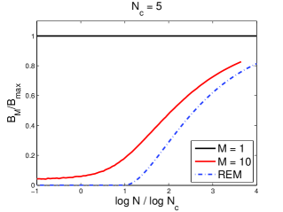
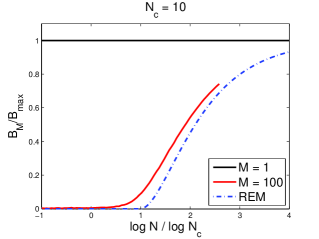
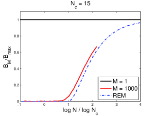
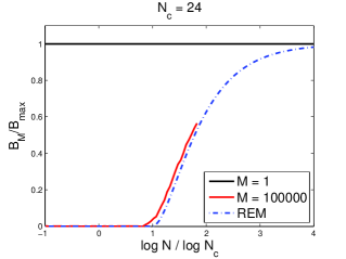
The results obtained in simulations of the adiabatic compression of a dilute real gas of $N$ particles in $d=3$ dimensions from a volume $V_{0}$ to a volume $V_{1}=V_{0}/4$ are shown in Figure 4. The plots display the normalized bias as a function of $\log N/\log N_{c}$ for different values of $M$, the number of measurements. In contrast with the Gaussian case, the curve for the random energy model changes, albeit slightly, as a function of $M$. The remaining curves in the plots correspond to averages over Monte Carlo simulations. The simulations cannot be performed for large values of $N$ because of numerical overflows. For fixed values of $M$, one observes a transition from a regime in which the bias is close to zero, for small systems, to a region in which the Jarzynski estimator is biased, when the system size is above a threshold $N_{c}$. The value of $N_{c}$ has a logarithmic dependence on $M$, which means that the change in regime occurs for fairly small systems, even when the number of experiments is rather large ($N_{c}\approx 24$ for $M=100,000$). Beyond this threshold, the bias increases monotonically and asymptotically approaches its maximum. The regime in which the bias is maximal corresponds to the realm of classical thermodynamics. Within this regime the measured work can be identified with either the average ($(Nd/2)\alpha$) or the typical value ($(Nd/2-1)\alpha$). Typical and average values of work, as well as the Jarzynski estimator in a finite number of measurements become indistinguishable as the number of gas particles increases.

The change between these two regimes, which is smooth for small $M$, becomes more abrupt as $M$ increases. The variant of the REM model analyzed in Appendix B provides a good qualitative description of the transition that becomes more accurate as $M$, $N$ and the volume change become larger.

V Discussion and conclusions

There are two paradigms in which statistical mechanics has successfully bridged mechanical and thermodynamic laws in systems composed of large numbers of particles using a probabilistic description. On the one hand, individual macroscopic systems can be characterized by the values of thermodynamic quantities and their fluctuations. In these large systems the distribution of each of the thermodynamic quantities is sharply peaked around its mode. Therefore, the fluctuations are small and need to be probed by means of special experimental techniques (e.g. light scattering for mass density fluctuations) or in indirect measurements (e.g. using fluctuation-dissipation relations to analyze the relaxation of systems removed from equilibrium). The most probable value obtained in a single experiment agrees with the average over several experiments. On the other hand, in a small system coupled to a large number of degrees of freedom the standard thermodynamic description is valid for the system plus environment considered as a whole. However, measurements of reduced properties associated with a small number of degrees of freedom are dominated by fluctuations. In consequence, thermodynamic relations cannot be used to describe individual measurements. Notwithstanding, they can be understood in terms of averages and fluctuations over repeated measurements. The coupling of the small system to the environment provides a mechanism for the reduced properties to approach their equilibrium values as given by the corresponding ensemble average Prigogine and Henin (1960); Henin et al. (1961); Ronis and Oppenheim (1977); Oppenheim (1989). Each measurement can be understood as sampling the initial state from the equilibrium distribution for the appropriate constraints (e.g. temperature, if the environment acts as a thermal reservoir). For standard thermodynamic quantities, these measurements over ensembles of small systems yield typical and average values that are close to each other. In contrast, typical values obtained in individual measurements of work in nonequilibrium processes do not fulfill the Jarzynski equality. In this equality, the average of the exponential of minus the work is computed by taking the mean of repeated independent measurements in systems prepared at equilibrium. By the law of large numbers, this Monte Carlo estimate converges to the expected value in the limit of an infinite number of measurements. However, the sum is dominated by rare events that need to be sufficiently well sampled so that the Monte Carlo estimate is close to the asymptotic result. If the number of samples is below a certain threshold, the estimator is biased. It becomes unbiased only for sufficiently large sample sizes. In the appropriate scaling limit, the change of behavior corresponds to a phase transition in variants of the random energy model, a simplified model for spin glasses.

This phenomenon can be analyzed from an alternative point of view. Assuming that the resources available are limited and that the number of measurements $M$ is fixed, the change of behavior in the estimator appears as the size of the system is increased. For small systems, the thermodynamic description needs to be understood in terms of ensemble averages, not of individual measurements. In this regime, the Jarzynski estimator is unbiased. It is equal to the exponential of minus the free energy difference in an isothermal evolution between the initial and the final values of the work parameter, independently of other characteristics of the actual nonequilibrium process that takes place in the system. In particular, it does not depend on the final state of the system after the external manipulation is completed. The lack of sensitivity to the details of the manipulation is a striking reflection at the microscopic level of the Hamiltonian evolution of the system as a whole (including the degrees of freedom of the environment) as demonstrated in Jarzynski (2004). The mechanical character of the equality is also highlighted by the fact that the largest contributions to the average correspond to initial configurations of the system that are typical of the reverse process Jarzynski (2006). Since these configurations need to be sufficiently well sampled, this implies that, under these conditions, the arrow of time is only tenuously defined.

For large systems and fixed $M$, the Jarzynski estimator becomes biased. In fact, as the size of the system approaches infinity, the average of the exponential of minus the work values obtained in the nonequilibrium process approaches the exponential of minus the average work. Since the typical and the average are close to each other, a single experiment and an average over a number of experiments of the order of $M$ yield results that are equivalent within measurement errors. Furthermore, this average depends on the details of the external manipulation. These features are in agreement with the standard thermodynamic description of an individual macroscopic system: the dominant configurations, which are rare for the initial state but typical of the final equilibrium state, are never sampled. The sample mean is dominated by typical configurations, which are characteristic of the forward process. Therefore, in this regime, the arrow of time becomes well defined.

The necessary condition to observe a transition in the Jarzynski estimator is that $<W>$, the average work in the nonequilibrium process, be different from $\Delta F$, the isothermal free-energy change. If the non-equilibrium process is adiabatic, these quantities are different even when the external manipulation of the system is slow. This can be seen in section IV.3, which analyzes a quasi-static adiabatic volume change in a dilute gas. Another example is the adiabatic expansion of an ideal gas against a piston: The maximum bias $B_{max}=<W>-\Delta F$ is different from zero even when the velocity of the piston approaches 0 (see Figure 4 in Palmieri and Ronis (2007)). The situation is different for isothermal processes. In this case $<W>$ approaches $\Delta F$ in the limit of quasi-static driving. Therefore, in an isothermal process, one should expect a transition from a fast driving regime, in which the Jarzynski estimator of the free energy difference is biased, to a slow driving regime, in which the Jarzynski estimator is unbiased. Isothermal processes are currently under analysis.

The conclusions of this study are, of course, not new. The emergence of irreversibility and of a thermodynamic description in systems with many degrees of freedom is one of the central results of statistical mechanics Boltzmann (2003); Gibbs (1902); Khinchin (1949); Zwanzig (2001); Castiglione et al. (2008). The analysis carried out shows how, in the context of the Jarzynski equality, the emergence of this macroscopic picture can be understood in terms of a phase transition that appears in the proper scaling limit and when the measurement resources are limited as the size of the system increases.

Appendix A The random energy model

The random energy model (REM) was introduced in Derrida (1980, 1981) as a simplified model for spin glasses that captures many salient properties of these types of disordered systems. In the random energy model, the system has $M=2^{K}$ energy levels, $\left\{E_{i}\right\}_{i=1}^{M}$. These energy levels are independent identically distributed random variables sampled from a normal distribution

$$p(E)=\frac{1}{\sqrt{\pi K}}e^{-E^{2}/K}.$$ (60)

The canonical partition function for a particular system (i.e. for a particular realization of the $M$ energy levels) at temperature $\beta^{-1}$ is

$$Z_{M}(\beta)\equiv\sum_{i=1}^{2^{K}}e^{-\beta E_{i}}.$$ (61)

In the limit of large $K\rightarrow\infty$, the system undergoes a second order phase transition

$$\lim_{K\rightarrow\infty}\frac{1}{K}\mathbb{E}\left[\log Z_{M}(\beta)\right]=\left\{\begin{array}[]{ll}\frac{\beta^{2}}{4}+\log 2,&\beta\leq\beta_{c}\\ \beta\sqrt{\log 2},&\beta>\beta_{c}\end{array}\right.,$$ (62)

where $\beta_{c}=2\sqrt{\log 2}$.

To make the connection between the Gaussian REM and the empirical estimation of the free energy in a process in which the work distribution is Gaussian, $W_{m}\sim N\left(\left<W\right>,\sigma^{2}\right)$ we make the change of variables

$$W_{m} = \left<W\right>+\sqrt{\frac{2\log 2}{\log M}}\sigma E_{m}$$

$$E_{m} \sim N\left(0,\frac{\log M}{2\log 2}\right),$$ (63)

where we have used the fact that $K=\log M/\log 2$. In terms of these new variables

$$\left<e^{-W}\right>_{M}=\frac{1}{M}\sum_{m=1}^{M}e^{-W_{m}}=\frac{1}{M}e^{-\left<W\right>}\sum_{m=1}^{M}e^{-\sqrt{\frac{2\log 2}{\log M}}\sigma E_{m}}.$$ (64)

Identifying $\sqrt{\frac{2\log 2}{\log M}}\sigma$ with $\beta$ in the REM, we obtain

$$\mathbb{E}\left[\Delta F_{M}\right] = -\mathbb{E}\left[\log\left<e^{-W}\right>_{M}\right]=\left<W\right>+\log M-\mathbb{E}\left[\log\left(\sum_{m=1}^{M}e^{-\sqrt{\frac{2\log 2}{\log M}}\sigma E_{m}}\right)\right]$$ (67)

$$= \left\{\begin{array}[]{ll}\left<W\right>-\frac{1}{2}\sigma^{2},&M\geq\exp\left\{\frac{1}{2}\sigma^{2}\right\}\\ \left<W\right>-\sqrt{2}\sigma\sqrt{\log M}+\log M,&M<\exp\left\{\frac{1}{2}\sigma^{2}\right\}\end{array}\right.$$

for $M\rightarrow\infty$ and $\sigma^{2}\rightarrow\infty$ with $\log M/\sigma^{2}\rightarrow\hbox{constant}$.

Appendix B The random energy model with energy levels that follow a gamma distribution

Consider a system with $M$ random energy levels, $\left\{E_{i}\right\}_{i=1}^{M}$, independently sampled from a gamma distribution

$$p(E)=\frac{\left(E+K\right)^{K-1}}{\Gamma(K)}e^{-\left(E+K\right)},\quad E\in[-K,\infty).$$ (68)

Define the parameter $\xi=\frac{\log M}{K\log 2}$. In terms of this parameter $M=2^{\xi K}$. It is possible to derive an expression for the entropy in the limit $K\rightarrow\infty$ by analyzing the behavior of ${\cal N}(\epsilon,\epsilon+\delta)$, the number of energy levels in an interval ${\cal I}(\epsilon;\delta)=\left[K\epsilon,K(\epsilon+\delta)\right]$, with $\epsilon\geq-1$, $\delta>0$ Mézard and Montanari (2009). Since this count depends on the realization of the system, ${\cal N}(\epsilon,\epsilon+\delta)$ is a binomial random variable whose first two moments are

$$\mathbb{E}\left[{\cal N}(\epsilon,\epsilon+\delta)\right] = 2^{\xi K}{\cal P}_{\cal I}(\epsilon;\delta)$$ (69)

$$\hbox{Var}\left[{\cal N}(\epsilon,\epsilon+\delta)\right] = 2^{\xi K}{\cal P}_{\cal I}(\epsilon;\delta)\left(1-{\cal P}_{\cal I}(\epsilon;\delta)\right),$$ (70)

where

$${\cal P}_{\cal I}(\epsilon;\delta)=\frac{K^{K}}{\Gamma(K)}\int_{\epsilon}^{\epsilon+\delta}(x+1)^{K-1}e^{-K(x+1)}dx$$ (71)

is the probability of an individual energy level to be in the interval ${\cal I}(\epsilon;\delta)$. As $K\rightarrow\infty$ these moments can be approximated to leading exponential order as

$$\mathbb{E}\left[{\cal N}(\epsilon,\epsilon+\delta)\right] \doteq \exp\left\{K\max_{[\epsilon,\epsilon+\delta]}s_{a}(x)\right\}$$ (72)

$$\frac{\hbox{Var}\left[{\cal N}([\epsilon,\epsilon+\delta])\right]}{\left[\mathbb{E}\left[{\cal N}(\epsilon,\epsilon+\delta)\right]\right]^{2}} \doteq \exp\left\{-K\max_{[\epsilon,\epsilon+\delta]}s_{a}(x)\right\}$$ (73)

with

$$s_{a}(x)=\xi\log 2+\log(1+x)-x.$$ (74)

Note that $s_{a}(x)\geq 0$ for $x_{l}\leq x\leq x_{u}$, where $-1\leq x_{l}\leq 0\leq x_{u}$ fulfill $s_{a}(x_{l})=s_{a}(x_{u})=0$. The limiting behavior of this equation when $\xi\rightarrow 0$ is

$$s_{a}(x)=\xi\log 2-x^{2}/2\quad x_{l}\leq x\leq x_{u},$$ (75)

where $x_{l}\approx-\sqrt{2\xi\log 2}$ and $x_{u}\approx\sqrt{2\xi\log 2}$. In this limit the results are similar to the Gaussian REM. In the opposite limit, when $\xi\rightarrow\infty$ is

$$s_{a}(x)=\xi\log 2+log(1+x),\quad x\approx x_{l},$$ (76)

where $x_{l}\approx-1+2^{-\xi}$.

The entropy function is defined as

$$s(\epsilon)=\left\{\begin{array}[]{ll}s_{a}(x)=\xi\log 2+\log(1+x)-x,&\quad x_{l}\leq x\leq x_{u}\\ -\infty,&\quad x<x_{l},x>x_{u}.\end{array}\right.$$ (77)

It can be shown that for any pair $\epsilon$, $\delta$, with probability one,

$$\lim_{K\rightarrow\infty}\frac{1}{K}\log{\cal N}(\epsilon,\epsilon+\delta)=\sup_{[\epsilon,\epsilon+\delta]}s(x).$$ (78)

The canonical partition function for a particular realization of the $M$ energy levels at temperature $\beta^{-1}$ is

$$Z_{M}(\beta)=\sum_{i=1}^{2^{\xi K}}e^{-\beta E_{i}}.$$ (79)

In the limit $K\rightarrow\infty$,

$$Z_{M}(\beta)\doteq\int_{x_{l}}^{x_{u}}\exp\left[K\left(s_{a}(x)-\beta x\right)\right]dx\doteq\exp\left[K\max_{x\in[x_{l},x_{u}]}\left(s_{a}(x)-\beta x\right)\right]$$ (80)

to exponential accuracy. Depending on the temperature, the maximum is either in the interval $(x_{l},0)$ (high temperature) or at $x_{l}$ (low temperature)

$${\arg\max}_{x\in[x_{l},x_{u}]}\left(s_{a}(x)-\beta x\right)=\left\{\begin{array}[]{ll}-\frac{\beta}{1+\beta},&\beta\leq\beta_{c}\\ x_{l},&\beta>\beta_{c}\end{array}\right.,$$ (81)

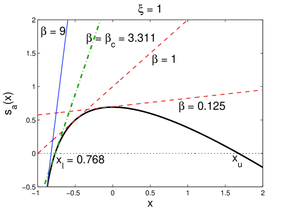
where $\beta_{c}=-x_{l}/(1+x_{l})$. A graphical construction that illustrates this transition is presented in figure (5) for $\xi=1$. The curves displayed are $s_{a}(x)$ and straight lines with slope $\beta$ that are tangent to $s_{a}(x)$ at the points that are local maxima of $s_{a}(x)-\beta x$. For high temperatures ($\beta\leq\beta_{c}$) the local maximum is within the interval $[x_{l},x_{u}]$ and is therefore the solution of (81). At low temperatures ($\beta>\beta_{c}$), the solution to (81) is $x_{l}$, which, in this regime, is a global maximum, but not a local one.

Figure 5: Transition between the low and high temperature regimes in the random energy model with energy levels sampled from a Gamma distribution (see text for details).

.

Using these relations it can be shown that, in this limit, the system undergoes a second order phase transition

$$\lim_{K\rightarrow\infty}\frac{1}{K}\mathbb{E}\left[\log Z_{M}(\beta)\right]=\left\{\begin{array}[]{ll}\xi\log 2+\beta-log(1+\beta),&\beta\leq\beta_{c}\\ -\beta x_{l}=\beta\beta_{c}/(1+\beta_{c}),&\beta>\beta_{c}\end{array}\right..$$ (82)

Continuity at $\beta_{c}$ implies that

$$log(1+\beta_{c})-\frac{\beta_{c}}{1+\beta_{c}}=\xi\log 2.$$ (83)

Consider now a sample of $M=2^{\xi K}$ work values $\left\{W_{m}\right\}_{m=1}^{M}$ from the distribution

$$p(W)=\frac{1}{\left|\alpha\right|\Gamma(K)}\left(\frac{W}{\alpha}\right)^{K-1}e^{-W/\alpha}\theta(\alpha W),$$ (84)

with $K=Nd/2$. The connection with the variant of REM analyzed in this section is achieved by making the change of variable

$$W_{m} = \left<W\right>+\alpha E_{m}\quad m=1,\ldots,M,$$ (85)

where $\left<W\right>=N\frac{d}{2}\alpha$ is the average work and $E_{m}$ are iidrvs sampled from the distribution (68). In terms of these new variables

$$\left<e^{-W}\right>_{M}=\frac{1}{M}\sum_{m=1}^{M}e^{-W_{m}}=\frac{1}{M}e^{-\left<W\right>}\sum_{m=1}^{M}e^{-\alpha E_{m}}.$$ (86)

Identifying $\alpha$ with $\beta$ in the random energy model, we conclude that there is an abrupt change of behavior of the Jarzynski estimator of the free energy differences for $M\rightarrow\infty$, $N\rightarrow\infty$ with $\log M/N\rightarrow\hbox{constant}$, as a function of $\xi=\frac{2\log M}{Nd\log 2}$

$$\mathbb{E}\left[\Delta F_{M}\right] = -\mathbb{E}\left[\log\left<e^{-W}\right>_{M}\right]=\left<W\right>+\log M-\mathbb{E}\left[\log\sum_{m=1}^{M}e^{-\alpha E_{m}}\right]$$ (89)

$$= \left\{\begin{array}[]{ll}N\frac{d}{2}log(1+\alpha),&\xi\geq\xi_{c}\\ N\frac{d}{2}\alpha(1+x_{l}(\xi))+\log M,&\xi<\xi_{c}\end{array}\right.,$$

where

$$\xi_{c}=\frac{\log(1+\alpha)-\frac{\alpha}{1+\alpha}}{\log 2}.$$ (90)

and $x_{l}(\xi)$ is the negative solution of the nonlinear equation

$$x_{l}(\xi)-\log(1+x_{l}(\xi))=\xi\log 2,\quad-1<x_{l}(\xi)<0.$$ (91)

At the transition point $\xi=\xi_{c}$

$$x_{l}(\xi_{c})=-\frac{\alpha}{1+\alpha}.$$ (92)

For a fixed number of particles $N$, the transition takes place when the number of measurements is above the threshold

$$M_{c}=\exp\left[N\frac{d}{2}\left(\log(1+\alpha)-\frac{\alpha}{1+\alpha}\right)\right].$$ (93)

Alternatively, for fixed number of experiments $M$, the transition occurs when the number of particles in the gas is below

$$N_{c}=\frac{2\log M}{d\left(\log(1+\alpha)-\frac{\alpha}{1+\alpha}\right)}.$$ (94)

Appendix C The discrete random energy model

Consider a system with $M=2^{K}$ energy levels, $\left\{E_{i}\right\}_{i=1}^{M}$. These energy levels are independent identically distributed random variables sampled from a binomial distribution

$$p(E)=\frac{1}{2^{N}}\binom{N}{\frac{1}{2}N+E},\quad E=-\frac{N}{2},-\frac{N}{2}+1,\ldots,\frac{N}{2}.$$ (95)

The canonical partition function at temperature $\beta^{-1}$ is

$$Z_{M}(\beta)=\sum_{i=1}^{2^{K}}e^{-\beta E_{i}}.$$ (96)

In the limit

$$M\rightarrow\infty\quad N\rightarrow\infty,\quad\gamma=\frac{K}{N}=\frac{\log M}{N\log 2}\rightarrow\hbox{constant}$$ (97)

the system undergoes a second order phase transition Ogure and Kabashima (2009)

$$\mathbb{E}\left[\log Z_{M}(\beta)\right]=\mathbb{E}\left[\log\left(\sum_{i=1}^{2^{K}}e^{-\beta E_{i}}\right)\right]=\left\{\begin{array}[]{ll}K\log 2+N\log\cosh\frac{\beta}{2},&\beta\leq\beta_{c}\\ \frac{1}{2}\beta N\tanh\frac{\beta_{c}}{2},&\beta>\beta_{c}\end{array}\right.$$ (98)

where

$$\beta_{c}=\left\{\begin{array}[]{ll}\infty,&\gamma\geq 1\\ \log\left[1-h_{2}^{-1}(1-\gamma)\right]-\log\left[h_{2}^{-1}(1-\gamma)\right],&\gamma<1\end{array}\right.$$ (99)

and the function $h_{2}^{-1}(y)\in[0,1/2]$ is the inverse of the binary entropy

$$h_{2}(x)=-x\log_{2}x-(1-x)\log_{2}(1-x).$$ (100)

To make the connection with the ideal gas compression experiment in the calculation of

$$\mathbb{E}\left[\Delta F_{M}\right]=-\mathbb{E}\left[\log\left<e^{-W}\right>_{M}\right]=-\mathbb{E}\left[\log\left(\frac{1}{M}\sum_{m=1}^{M}e^{-n_{m}\epsilon}\right)\right],$$ (101)

where $n_{m}\in\left\{0,1,\ldots N\right\}$ follows a binomial distribution of parameters $N$, $p(0)=1/2$, we make the change of variable

$$n_{m}=\frac{1}{2}N+E_{m};\quad E_{m}\in\left\{-\frac{N}{2},-\frac{N}{2}+1,\ldots\frac{N}{2}\right\}.$$ (102)

Using these new random variables

$$\mathbb{E}\left[\Delta F_{M}\right] = -\mathbb{E}\left[\log\left(e^{-\frac{1}{2}N\epsilon}\frac{1}{M}\sum_{m=1}^{M}e^{-E_{m}\epsilon}\right)\right]$$ (103)

$$= N\frac{\epsilon}{2}+\log M-\mathbb{E}\left[\log\left(\sum_{m=1}^{M}e^{-E_{m}\epsilon}\right)\right].$$

Finally, identifying $\epsilon$ with $\beta$ in the DREM, and $\epsilon_{c}=\beta_{c}$

$$\mathbb{E}\left[\Delta F_{M}\right]=\left\{\begin{array}[]{ll}N\left[\frac{\epsilon}{2}-\log\cosh\frac{\epsilon}{2}\right]=N\log\frac{2}{1+e^{-\epsilon}},&\epsilon\leq\epsilon_{c}\\ N\left[\gamma\log 2+\frac{\epsilon}{2}\left(1-\tanh\frac{\epsilon_{c}}{2}\right)\right],&\epsilon>\epsilon_{c}\end{array}\right.,$$ (104)

where we have used that fact that $K=\log M/\log 2$ and $\gamma=K/N=\frac{\log M}{N\log 2}$.