The Acceleration of Ions in Solar Flares During Magnetic Reconnection

Abstract

The acceleration of solar flare ions during magnetic reconnection is explored via particle-in-cell simulations that self-consistently and simultaneously follow the motions of both protons and $\alpha$ particles. We show that the dominant heating of thermal ions during guide field reconnection, the usual type in the solar corona, results from pickup behavior during the entry into reconnection exhausts. In contrast to anti-parallel reconnection, the temperature increment is dominantly transverse, rather than parallel, to the local magnetic field. A comparison of protons and alphas reveals a mass-to-charge ($M/Q$) threshold in pickup behavior that favors heating of high-$M/Q$ ions over protons, which is consistent with impulsive flare observations.

1 INTRODUCTION

The generation of energetic particles during flares remains a central unsolved issue in solar physics. Extensive observational evidence indicates that a substantial fraction of the energy released during a flare rapidly accelerates charged particles, with electrons reaching $\mathcal{O}(1)$ MeV and ions $\mathcal{O}(1)$ GeV/nucleon (Emslie et al., 2004). Explaining this energization requires accounting not only for the relevant energy and time scales but also the resulting spectra, which exhibit a common shape for almost all ion species. At the same time, high mass-to-charge ($M/Q$) ions are greatly over-represented in flares, with abundances as much as two orders of magnitude higher than normal coronal values (Mason et al., 1994; Mason, 2007).

In impulsive flare models, magnetic reconnection is the ultimate energy source, and so it is natural to consider theories in which reconnection also plays a role in particle acceleration. Some models, including those that rely on interactions with magnetohydrodynamic (MHD) waves (Miller, 1998; Petrosian & Liu, 2004) or shock acceleration (Ellison & Ramaty, 1985; Somov & Kosugi, 1997), use reconnection only as an indirect source that provides an environment in which other energization processes can occur. In other models, the magnetic energy released during reconnection is more directly channeled to particles through various processes — DC electric fields (Holman, 1985), interactions with multiple magnetic islands (Onofri et al., 2006), first-order Fermi acceleration (Drake et al., 2010), or the pickup of collisionally ionized neutrals (Wu, 1996).

Also a member of this latter group is the direct heating of ions in reconnection exhausts (Krauss-Varban & Welsch, 2006; Drake et al., 2009b), in which the perpendicular and parallel (relative to the magnetic field) temperatures of ions jump after traversing the narrow boundary layer separating the ions that flow slowly in from upstream from the reconnection exhaust, which travels at the Alfvén speed $B/\sqrt{4\pi\rho}$ where $B$ is the strength of the magnetic field and $\rho$ is the density. However these works considered the weak guide field limit in which ion heating is parallel, rather than transverse, to the local magnetic field; Cranmer & van Ballegooijen (2003) have shown that in the extended solar corona, $T_{\perp}\gg T_{\parallel}$. Subsequently, Drake et al. (2009a) used test particles in a Hall MHD simulation with a large guide field (five times larger than the reconnecting field) to confirm that ions above a critical value of $M/Q$ become demagnetized. They suggested that ions crossing into reconnection outflows can become non-adiabatic, and hence behave like pickup particles (Möbius et al., 1985), while gaining an effective thermal velocity equal to the Alfvén speed and derived a $M/Q$-based threshold for this behavior. This process is similar to an earlier proposal by Wu (1996) that ion acceleration in impulsive flares can occur via reconnection-associated pickup, although in that case the accelerated ions were produced by neutral-particle ionization in the lower corona. Later hybrid simulations by Wang et al. (2001) confirmed that injected protons (mimicking newly ionized particles) did behave like pickup particles in this scenario.

In this Letter, we use a kinetic particle-in-cell (PIC) simulation to track two types of ions self-consistently, i.e. without resorting to test particles, to determine whether particles above the critical value of $M/Q$ behave like pickup particles in dynamic electromagnetic fields. Ions with $M/Q$ below the threshold derived in Drake et al. (2009a) (protons, in this case) are adiabatic and undergo very little heating as they move between the upstream plasma and the reconnection exhaust, while particles above the threshold ($\alpha$ particles) gain an effective thermal velocity equal to the exhaust velocity after crossing the narrow boundary layer surrounding the exhaust.

The transition between adiabatic and non-adiabatic behavior depends on the ratio between a particle’s cyclotron period and the the time it takes to cross the boundary layer (Drake et al., 2009a). An adiabatic particle turns sharply in the outflowing direction upon entering the exhaust, conserving its magnetic moment $\mu=m\delta v_{\perp}^{2}/2B$, where $\delta v_{\perp}$ is the ion perpendicular velocity with the $\mathbf{E}\bm{\times}\mathbf{B}$ contribution subtracted (the ion perpendicular velocity is taken relative to $\mathbf{B}$). However, particles which behave non-adiabatically move in the direction of the local electric field upon entering the exhaust and not in the direction of the local $\mathbf{E}\bm{\times}\mathbf{B}$ velocity. The sudden change from slow upstream inflow to downstream Alfvénic outflow causes particles with high $M/Q$ to see a jump in their magnetic moments.

2 NUMERICAL SIMULATIONS

We carry out simulations using the code p3d (Zeiler et al., 2002). Like all PIC codes, it tracks individual particles ($\approx 10^{9}$ in this work) as they move through electromagnetic fields that are defined on a mesh. Unlike more traditional fluid representations (e.g., MHD), PIC codes correctly treat small lengthscales and fast timescales, which are particularly important for understanding the x-line and separatrices during magnetic reconnection.

The simulated system is periodic in the $x-y$ plane, where flow into and away from the x-line are parallel to $\mathbf{\hat{y}}$ and $\mathbf{\hat{x}}$, respectively, and the guide magnetic field and reconnection electric field parallel $\mathbf{\hat{z}}$. The initial magnetic field and density profiles are based on the Harris equilibrium (Harris, 1962). The reconnecting magnetic field is given by $B_{x}=\tanh[(y-L_{y}/4)/w_{0}]-\tanh[(y-3L_{y}/4)/w_{0}]-1$, where $w_{0}$ and $L_{y}$ are the half-width of the current sheets and the box size in the $\mathbf{\hat{y}}$ direction. The density comprises an ambient background and two current sheets in which the density rises in order to maintain pressure balance with the magnetic field. We initiate reconnection with a small initial magnetic perturbation that produces a single magnetic island on each current layer.

The code is written in normalized units in which magnetic fields are scaled to the asymptotic value of the reversed field $B_{0x}$, densities to the value at the center of the reconnecting current sheet minus the uniform background density, velocities to the proton Alfvén speed $c_{A}=B_{0x}/\sqrt{4\pi m_{p}n_{0}}$, times to the inverse proton cyclotron frequency in $B_{0x}$, $\Omega_{px}^{-1}=m_{p}c/eB_{0x}$, lengths to the proton inertial length $d_{p}=c_{A}/\Omega_{px}$ and temperatures to $m_{p}c_{A}^{2}$.

The proton to electron mass ratio is taken to be $25$, in order to minimize the difference between pertinent length scales and hence run as large a simulation domain as possible. It has been shown (Shay et al., 1998; Hesse et al., 1999; Shay et al., 2007) that the rate of magnetic reconnection and structure of the outflow exhaust do not depend on this ratio, and neither, therefore, does the ion heating examined here, which depends only on the exhaust geometry. The simulation assumes $\partial/\partial z=0$, i.e. that field and particle quantities do not vary in the out-of-plane direction, making this a two-dimensional simulation.

In addition to the usual protons and electrons, we also include a number density of $1\%$ ⁴He⁺⁺ ($\alpha$) particles in the background particle population and gave them an initial temperature equal to that of the protons. This number density does not affect the reconnection dynamics appreciably, while still providing a large sample of particles with $M/Q>1$, where $M/Q$ is normalized to the proton value. Each particle (protons and $\alpha$’s) is assigned a unique tag number, allowing individual particles to be tracked throughout the simulation.

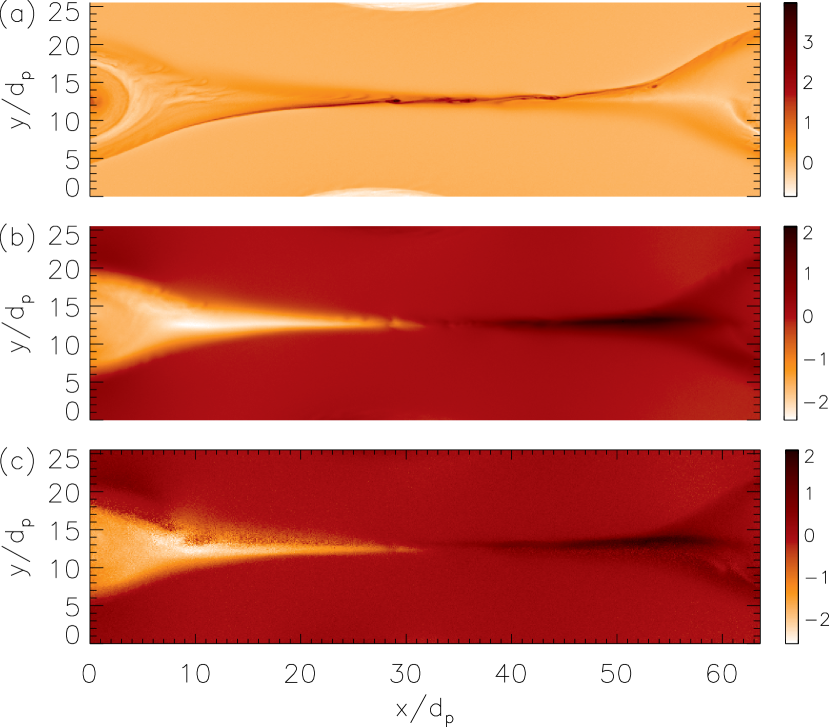
Figure 1: Overview of a PIC simulation with an initial guide field $B_{0z}=2B_{0x}$. Panel (a): the total out-of-plane current density $J_{z}$; panel (b): the proton outflow velocity $v_{px}$; panel (c): the $\alpha$ particle outflow velocity $v_{\alpha x}$

In Fig. 1 we show an overview of results from a simulation with a computational domain $L_{x}\times L_{y}=102.4\times 51.2\,d_{p}$ and an initial guide field $B_{0z}=2.0B_{0x}$ at $t=200\Omega_{px}^{-1}$. The grid spacing for this run is $0.025\,d_{p}$, the electron, proton, and $\alpha$ temperatures, $T_{e}=T_{p}=T_{\alpha}=0.25m_{p}c_{A}^{2}$, are initially uniform and the velocity of light is $15c_{A}$. The half-width of the initial current sheet, $w_{0}$, is $1\,d_{p}$ and the background density is $0.2$. Panel (a) depicts the total out-of-plane current density $J_{z}$ centered around the x-line (at $x/d_{p}\approx 32$ and $y/d_{p}\approx 13$) of one of the current sheets. Magnetic field lines (not shown) roughly trace contours of $J_{z}$.

Ambient plasma from above and below the current sheet slowly flows toward the current sheet while embedded in oppositely directed magnetic field (to the right above the layer, to the left below). Reconnected field lines are highly bent and, to reduce their magnetic tension, rapidly move away from the x-line, dragging plasma with them. Panels (b) and (c) show the proton and $\alpha$ outflow velocities $v_{px}$ and $v_{\alpha x}$. The similarity between the two makes it clear that both the protons and the $\alpha$’s participate in the reconnection outflow which, outside of the immediate vicinity of the X-line, has a magnitude of $v_{x}\sim cE_{y}/B_{z}\sim c_{A}$ ($\approx 1$, in our normalized units). A comparison of Fig. 1 to frames (a) and (b) of Fig. 1 in Drake et al. (2009a) (which shows results from a run otherwise identical but for the presence of the $\alpha$ particles) demonstrates that the $\alpha$’s do not significantly change the structure of the reconnection exhaust.

3 ION PICKUP AND HEATING

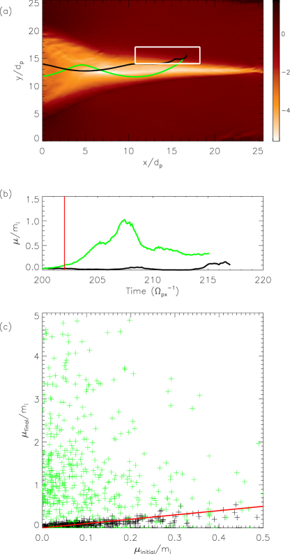
Figure 2: Panel (a): Trajectories for a proton (black) and $\alpha$ particle (green) randomly picked from a $7.5\times 3\,d_{p}$ box (shown in white) are overlaid on a snapshot of $E_{y}$. Panel (b): The magnetic moment per mass as a function of time for the two particles in (a). The red line represents the time of the snapshot of $E_{y}$. Panel (c): For 500 protons (black) and 500 $\alpha$’s (green) selected at random from the white box in (a), their final magnetic moments plotted against their initial magnetic moments. The red line has unit slope and represents the expected result if $\mu/m$ were invariant.

Particle acceleration is controlled by the structure and magnitude of the electric field. During reconnection a strong transverse electric field $E_{y}=-E_{z}B_{0z}/B_{y}$ develops in the exhaust to force $\mathbf{E}\cdot\mathbf{B}=0$; its structure to the left of the x-line is shown in the background of Fig. 2(a). Particles enter the exhaust with a velocity $v_{y}\sim 0.1c_{A}$. Any energy gain is determined by whether particles crossing the exhaust boundary, which has scale length given by the ion sound Larmor radius $\rho_{s}$ ($=v_{s}/\Omega_{p}$, where $v_{s}$ is the plasma sound speed), are adiabatic. Non-adiabatic particles cross the boundary in a time $\tau_{c}$ that is short compared with their cyclotron period, $\tau_{c}\approx\rho_{s}/v_{y}\approx 10\rho_{s}/c_{A}<\pi/\Omega_{px}$, or

$$\frac{M}{Q}>\left(\frac{5\sqrt{2}}{\pi}\right)\sqrt{\beta_{px}}$$ (1)

where $\beta_{px}=8\pi nT/B_{0x}^{2}$ (Drake et al., 2009a). Thus, in the present simulations, where the upstream $\beta_{px}=0.2$, equation 1 gives $M/Q>1$ for non-adiabatic behavior and so protons are marginally adiabatic while $\alpha$’s ($M/Q=2$) are not. Since $E_{y}<0$ in this case, non-adiabatic positively charged ions entering the exhaust from below will be pushed out immediately, preventing them from being caught up in the exhaust. However, non-adiabatic positively charged ions entering from the top will find themselves essentially at rest in the simulation frame while the outflow moves past at roughly the Alfvén speed. Such particles will undergo an $\mathbf{E}\bm{\times}\mathbf{B}$ drift, but with a “thermal velocity” equal to the Alfvén speed and have trajectories resembling cycloids. This process is analogous to that undergone by stationary neutral atoms surrounded by the moving solar wind. If ionized, the new ion first moves in the direction of the motional electric field in order to gain the necessary energy to flow with the rest of the wind. As it gets “picked up”, it gains a thermal velocity equal to the solar wind velocity (Möbius et al., 1985).

We randomly selected 500 protons and 500 $\alpha$ particles from the $7.5\,d_{p}\times 3\,d_{p}$ box upstream of the exhaust shown in Fig. 2(a) at $t=200\Omega_{px}^{-1}$ and followed their trajectories for 25 $\Omega_{px}^{-1}$. In Fig. 2(a) we plot a representative trajectory for a proton, shown in black, and an $\alpha$ shown in green, over a background of $E_{y}$. (Note that the overlaid trajectories in (a) are calculated in the fully self-consistent simulation, while the background of $E_{y}$ is a snapshot from $t=202\,\Omega_{px}^{-1}$.) The proton, which remains adiabatic, immediately moves downstream upon entering the exhaust, while the $\alpha$ particle moves in the direction of $E_{y}$ before being picked up by the $\mathbf{E}\bm{\times}\mathbf{B}$ drift. Panel (b) displays the time evolution of the proton (black) and $\alpha$ (green) magnetic moments (scaled by mass). The vertical red line corresponds to the time at which $E_{y}$ is shown in (a). After crossing the boundary layer into the exhaust, the $\alpha$ becomes demagnetized, as indicated by the jump in $\mu$, a trend seen for all of the tracked $\alpha$’s. In (c) we plot the magnetic moments of all 500 protons (black) and all 500 $\alpha$’s (green) after entering the exhaust versus their moments at $t=200\Omega_{px}^{-1}$. For each particle $\mu_{\text{final}}$ was measured when the particle crossed a specified horizontal position at the downstream edge of the exhaust, around $6\,d_{p}$ in Fig. 2(a). For reference, we overplot a line of unit slope, which corresponds to exact $\mu$ conservation. The clustering of protons near this line and large values of $\mu/m$ reached by the $\alpha$’s clearly shows the adiabatic nature of the former and the non-adiabatic nature of the latter.

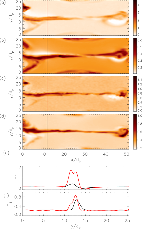
Figure 3: Spatially smoothed temperature components at $t=200\Omega_{px}^{-1}$. Panel (a): $T_{\perp}$ for $\alpha$ particles; panel (b): $T_{\perp}$ for protons; panel (c): $T_{\parallel}$ for $\alpha$’s; panel (d): $T_{\parallel}$ for protons. Panels (e) and (f): Cuts through the exhaust of the perpendicular and parallel components, respectively, for $\alpha$’s (red) and protons (black). The locations of the cuts are shown by the vertical lines in (a)-(d).

In Fig. 3 we show the temperatures of both species. Panels (a) and (b) depict the perpendicular (to the magnetic field) $\alpha$ and proton temperatures, while (c) and (d) show the parallel temperatures. The $\alpha$ temperature increase is greater than the proton temperature in the perpendicular direction (note the different color bar scales in the two panels). Indeed, the temperature increase of the $\alpha$’s is more than mass proportional, consistent with observations (Cranmer & van Ballegooijen, 2003). This is also evident in frames (e) and (f), which are cuts through the perpendicular and parallel temperature plots for the $\alpha$’s (red) and protons (black). The weak heating of the protons is consistent with the adiabatic behavior shown in Fig. 2. The analysis of Drake et al. (2009a) predicts that, with a guide field of $B_{0z}=2B_{0x}$, the proton temperature will change by

$$\Delta T_{\parallel}=\frac{B_{0x}^{2}}{B_{0z}^{2}}v_{x}^{2}\sim\frac{v_{x}^{2}}{4}\text{;}\qquad\Delta T_{\perp}=0$$ (2)

in the exhaust, and the $\alpha$ temperature will change by:

$$\Delta T_{\parallel}=0\text{;}\qquad\Delta T_{\perp}=\frac{1}{2}m_{\alpha}v_{x}^{2}\sim 2v_{x}^{2}.$$ (3)

For $v_{x}^{2}\sim 2$ (see Fig. 1) these jumps are in reasonable agreement with the observed variations. Differences from the predicted values, in particular the changes in $T_{\perp}$ for the protons and $T_{\parallel}$ for the $\alpha$’s, presumably arise from corrections to equations (2) and (3) due to a mixture of adiabatic and non-adiabatic behavior by the particles.

In Fig. 4, we show how the velocity distributions of the $\alpha$’s and protons change as they move from the upstream to the downstream region. Panels (a) and (d) depict the upstream $\alpha$ and proton velocity distribution in the $v_{x}-v_{y}$ plane. The protons and $\alpha$’s were given the same initial temperature, so upstream of the exhaust, the protons’ mean thermal velocity is higher than the $\alpha$ particles’. The small negative $v_{y}$ component upstream in both species shows the inflow toward the reconnection exhaust. After crossing the narrow boundary layer, the $\alpha$’s get picked up by the Alfvénic outflow (at this time the local density is $\sim$ 0.2, so the local Alfvén speed is $\sim\sqrt{5}$), and their thermal velocity increases much more than that of the adiabatic protons. The downstream velocity distributions for the $\alpha$’s and protons are shown in the $v_{x}-v_{y}$ plane in (b) and (e) and in the $v_{x}-v_{z}$ plane in (c) and (f), both calculated inside a box located between $5-12.5\,d_{p}$ in the x-direction and $11.4-13.4\,d_{p}$ in the y-direction. Since the dominant $\mathbf{B}$ component is the guide field, $v_{x}$ and $v_{y}$ are essentially perpendicular velocity components, and $v_{z}$ the parallel velocity. The protons exhibit very little heating in the $v_{x}-v_{y}$ plane (Fig. 4(e)), consistent with adiabatic behavior. They are modestly heated in the z-direction (Fig. 4(f)), consistent with $T_{\parallel}$ in Eq. 2. The $\alpha$ particles are strongly heated in the y-direction (Fig. 4(b)) and are beginning to form a ring distribution that is characteristic of pickup behavior. There is modest heating of $\alpha$ particles in the z-direction (Fig. 4(c)), but the similar structure in (c) and (f) suggests that the heating mechanism is the same for both protons and $\alpha$’s, and it is possible that the $\alpha$ particles are not completely non-adiabatic.

4 DISCUSSION

Using self-consistent tracking of particle trajectories, we have shown that ions above a critical mass-to-charge threshold (Drake et al., 2009a) behave like pickup ions in reconnection exhausts, with $\mu$ changing due to a sharp increase in $v_{\perp}$. Ion energy increments of $\approx 25$ keV/nucleon are predicted for typical coronal parameters of $B=50$ G and $n=10^{9}/\text{cm}^{3}$. Ions below this threshold are only weakly heated. This transition only exists for reconnection with a guide field which, however, is the typical case in the solar corona. Coronal observations have revealed that the abundances of high mass-to-charge ions are enhanced in solar flares, with the strength of the enhancement depending only on $M/Q$. The fact that we observe non-adiabatic behavior and associated strong heating for particles with $M/Q>1$, while the proton heating remains weak, suggests that reconnection might explain the abundance enhancements in impulsive flares. Abundance enhancements should occur because high $M/Q$ ions are heated at lower values of the reconnecting magnetic field strength (see Eq. 1) than protons. Furthermore, the increase in $T_{\perp}/T_{\parallel}$ in the exhaust seen here is consistent with that observed in the extended solar corona (Cranmer & van Ballegooijen, 2003), although it should be noted that the number density of $\alpha$ particles used here is slightly less than what is observed in the corona ($n_{\alpha\text{,corona}}\sim 5\%-10\%$).

Observations near 1 AU of solar wind reconnection events with the Wind spacecraft (as, for example, in Phan et al. (2010)) should be able to measure $T_{\parallel}$ and $T_{\perp}$ for both protons and $\alpha$ particles in order to test the mechanism suggested in this work. Moreover, provided its instrumentation can differentiate between different $M/Q$ ions, the upcoming Solar Probe Plus mission, with a planned perihelion of $\approx 9R_{\odot}$ (which lies within the outer corona), should also provide an excellent test of these predictions.

Finally, it is widely believed that some process converts a fraction of the energy found in the convective motions of the solar photosphere into the heat that ensures the continuous existence of a $\mathcal{O}(10^{6}\text{ K})$ corona and accelerates the solar wind. Broadly speaking the two most likely candidates are wave heating — in which oscillations generated in the photosphere travel into the corona, develop into turbulence, and eventually dissipate — and magnetic reconnection, in which the topological reorganization of the magnetic field releases energy and heats the plasma.

Measurements by the Solar Ultraviolet Measurements of Emitted Radiation (SUMER) and Ultraviolet Coronal Spectrometer (UVCS) instruments of the SOHO (Solar and Heliospheric Observatory) spacecraft provide significant constraints on any theory of coronal heating. In particular, at heights of $2-3R_{\odot}$ protons have a slight temperature anisotropy (in the $T_{\perp}>T_{\parallel}$ sense) while heavier ions (represented by $O^{5+}$) are strongly anisotropic, with $T_{\perp}/T_{\parallel}\gtrsim 10$ (Cranmer & van Ballegooijen, 2003). Interestingly, the process discussed in this work should be active in the region in question and produces temperature anisotropies consistent with these results.

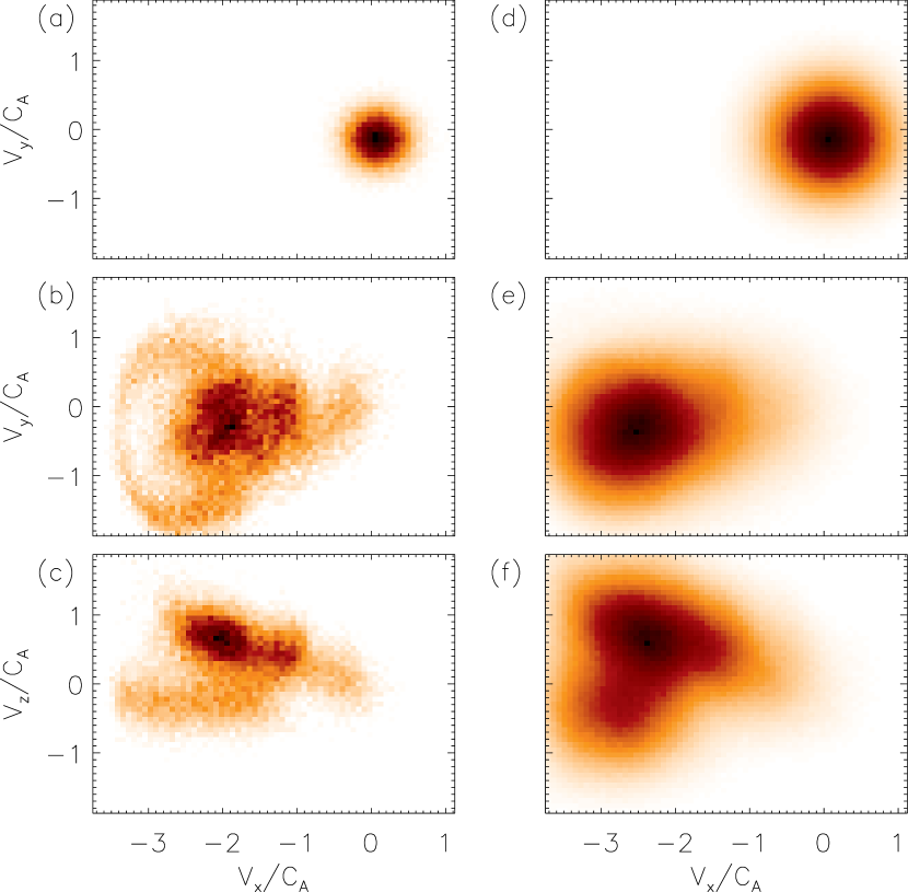
Figure 4: 2D velocity distribution functions upstream and downstream of the exhaust. Panels (a) and (d): upstream $v_{x}-v_{y}$ distributions for $\alpha$’s and protons, respectively. Panels (b) and (e): downstream $v_{x}-v_{y}$ distributions for $\alpha$’s and protons; panels (c) and (f): downstream $v_{x}-v_{z}$ distributions.

References

- Cranmer & van Ballegooijen (2003) Cranmer, S. R., & van Ballegooijen, A. A. 2003, Ap. J., 594, 573
- Drake et al. (2009a) Drake, J. F., Cassak, P. A., Shay, M. A., Swisdak, M., & Quataert, E. 2009a, Ap. J., 700, L16
- Drake et al. (2010) Drake, J. F., Opher, M., Swisdak, M., & Chamoun, J. N. 2010, Ap. J., 709, 963
- Drake et al. (2009b) Drake, J. F., et al. 2009b, J. Geophys. Res., 114
- Ellison & Ramaty (1985) Ellison, D. C., & Ramaty, R. 1985, Ap. J., 298
- Emslie et al. (2004) Emslie, A. G., et al. 2004, J. Geophys. Res., 109
- Harris (1962) Harris, E. G. 1962, Nuovo Cim., 23, 115
- Hesse et al. (1999) Hesse, M., Schindler, K., Birn, J., & Kuznetsova, M. 1999, Phys. Plasmas, 6, 1781
- Holman (1985) Holman, G. D. 1985, Ap. J., 293, 584
- Krauss-Varban & Welsch (2006) Krauss-Varban, D., & Welsch, B. T. 2006, Proceedings of the International Astronomical Union, 2, 89
- Mason (2007) Mason, G. M. 2007, Space Sci. Rev., 130, 231
- Mason et al. (1994) Mason, G. M., Mazur, J. E., & Hamilton, D. C. 1994, Ap. J., 425, 843
- Miller (1998) Miller, J. A. 1998, Space Sci. Rev., 86, 79
- Möbius et al. (1985) Möbius, E., Hovestadt, D., Klecker, B., Scholer, M., Gloeckler, G., & Ipavich, F. M. 1985, Nature, 318, 426
- Onofri et al. (2006) Onofri, M., Isliker, H., & Vlahos, L. 2006, Phys. Rev. Lett., 96
- Petrosian & Liu (2004) Petrosian, V., & Liu, S. 2004, Ap. J., 610, 550
- Phan et al. (2010) Phan, T. D., et al. 2010, Ap. J.. Lett., 719, L199
- Shay et al. (1998) Shay, M. A., Drake, J. F., Denton, R. E., & Biskamp, D. 1998, J. Geophys. Res., 103, 9165
- Shay et al. (2007) Shay, M. A., Drake, J. F., & Swisdak, M. 2007, Phys. Rev. Lett., 99
- Somov & Kosugi (1997) Somov, B. V., & Kosugi, T. 1997, Ap. J., 485, 859
- Wang et al. (2001) Wang, X. Y., Wu, C. S., Wang, S., Chao, J. K., Lin, Y., & Yoon, P. H. 2001, Ap. J., 547, 1159
- Wu (1996) Wu, C. S. 1996, Ap. J., 472, 818
- Zeiler et al. (2002) Zeiler, A., Biskamp, D., Drake, J. F., Rogers, B. N., Shay, M. A., & Scholer, M. 2002, J. Geophys. Res., 107, 1230