Reciprocity in quantum, electromagnetic and other wave scattering

Abstract

The reciprocity principle is that, when an emitted wave gets scattered on an object, the scattering transition amplitude does not change if we interchange the source and the detector – in other words, if incoming waves are interchanged with appropriate outgoing ones. Reciprocity is sometimes confused with time reversal invariance, or with invariance under the rotation that interchanges the location of the source and the location of the detector. Actually, reciprocity covers the former as a special case, and is fundamentally different from – but can be usefully combined with – the latter. Reciprocity can be proved as a theorem in many situations and is found violated in other cases. The paper presents a general treatment of reciprocity, discusses important examples, shows applications in the field of photon (Mössbauer) scattering, and establishes a fruitful connection with a recently developing area of mathematics.

I Introduction

Symmetry is a key notion in physics. In the field of natural sciences, symmetry can be interpreted as a concept of balance or patterned self-similarity Weyl (1983), regarding to concrete as well as abstract objects like a physical system itself or, for example, a theoretical model, respectively Mainzer (2005). According to the Oxford online dictionary, symmetry is a law or operation where a physical property or process has an equivalence in two or more directions, or events/actions are balanced/equal in some way. A synonym to the term symmetry is invariance, expressing the fact that a special operation (called symmetry transformation), which could be a change of some physical parameters – like a geometric transformation, a change of polarization, parity, charge, the arrow of time, etc. – does not change some particular property of the system. Depending on the studied system, symmetry may have various measures and operational definitions. In the theoretical model of quantum mechanics, symmetry transformations were given by Wigner (1959) as general operators preserving the modulus of scalar products of the vectors of the Hilbert space representing the physical states. Further, the symmetry theorem of Wigner (1959) states that any symmetry transformation can be represented by either a unitary linear or an isometric conjugate linear (usually called antiunitary) operator.

A large class of physical processes can be described in the framework of scattering theory Schiff (1968); Messiah (1968), which is a theoretical sub-model inside quantum mechanics, but can be interpreted in classical electrodynamics and in the classical mechanics of elastic waves as well. As documented in the literature since long ago, physical intuition suggests that, when reversing the position of source and detector in a wave scattering experiment (see Fig. 1), the observed signal will not change. This condition, called the reciprocity principle, is indeed fulfilled in most cases. Nevertheless, it does not follow directly from first principles, therefore, it is not necessarily fulfilled.

The physical term ‘reciprocity’ appeared already in the 19^th century. The first reciprocity equations related reflection and transmission of light at an interface between lossless optical media, and were derived by Stokes (1849). The principle of reciprocity was later generalized for more complex scattering systems in the field of electromagnetic waves von Helmholtz (1866); Lorentz (1905), sound waves Strutt and Rayleigh (1877), electric circuits Carson (1924), and radio communication Carson (1930), as well as in quantum mechanical scattering problems Bilhorn et al. (1964). The reciprocity related publications cover the whole 20^th century, as it is summarized in the review paper of Potton (2004). Reciprocity can be proven for various scattering problems with certain limits of validity Hoop (1959); Saxon (1955); Carminati et al. (2000); Hillion (1978).

The number of reciprocity related publications grew intensively in the last decade as well, and all the approaches that appeared earlier were subject to further developments. Among others, the reciprocity relations of Stokes (1849) were generalized to multilayers Vigoureux and Giust (2000) and to absorptive multilayers Gigli et al. (2001); André and Jonnard (2009). The applications in electrodynamics for electric circuits and antennas were studied by Sevgi (2010), and the reciprocity theorem of classical electrodynamics in case of material media containing linearly polarizable and linearly magnetizable substances was formulated by Mansuripur and Tsai (2011). Nonreciprocal devices (circulators and isolators) with on-chip integration possibility were recently suggested by Kamal et al. (2011). In parallel, reciprocity admits applications in particle scattering, acoustics, seismology, and the solution of inverse problems as well Potton (2004).

Reciprocity was considered for nonlocal electrodynamical Xie et al. (2009a, b) and nonlocal quantum mechanical systems Xie et al. (2008). In a recent publication of Leung and Young (2010), the aspect of gauge invariance was discussed from the point of view of quantum mechanical interpretation of reciprocity, and new gauge invariant formulations of reciprocity were suggested and analyzed.

What is reciprocity? In many works it is simply related to time reversal symmetry Mytnichenko (2005); Wurmser (1996) as was done in the well-known reciprocity theorem of Landau and Lifshitz (1981). The optical reciprocity theorem, however, revealed that absorption, which violates time reversal invariance, conserves reciprocity in polarization independent cases Born and Wolf (1999), which observation was also expressed in scattering theory Bilhorn et al. (1964). In parallel, according to the original reciprocity principle, namely, invariance under the interchange of source and detector, one could have the impression that reciprocity is identical to a rotation by $180^{\circ}$. However, this latter interpretation also proves false since there exist scatterers with no $180^{\circ}$ rotational symmetry but fulfilling the reciprocity principle.

The currently typically used condition of reciprocity in linear systems is the self-transpose (also called complex symmetric) property of the matrix of the scattering potential, of the index of refraction, of the dielectric/magnetic permeability tensors, or of the Green’s function Xie et al. (2009a, b). This condition, however, depends on the frame, on the polarization basis chosen. Indeed, applying a unitary basis transformation, the self-transpose property of the matrix is not conserved, as it can be demonstrated on the case of a Hermitian matrix, which is not self-transpose in general, but can be diagonalized – hence, the self-transpose form is obtained by an appropriate unitary transformation. In the light of this observation, the physical content of reciprocity seems to be unclear. Our main task is to give a proper frame-independent description of reciprocity, extending the excellent early work of Bilhorn et al. (1964).

The nonreciprocal properties of systems are even less understood. Magneto-optical systems are typically cited as nonreciprocal media Potton (2004); Kamal et al. (2011), but detailed analyses of the reasons of reciprocity violation have not been given.

Reciprocity violation can be obtained in case of magneto-optical gyrotropy Potton (2004), which is a well-known property of the Mössbauer medium Blume and Kistner (1968). At Mössbauer resonances, the ratio of the time-inversion-violating to normal potentials is typically of the order of one thousand! The resonant Mössbauer medium is absorptive and gyrotropic and, accordingly, for well-defined geometrical situations, significant reciprocity violation is expected.

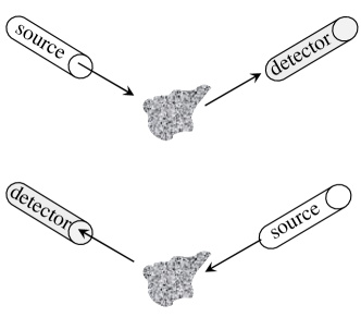
Figure 1: Scattering experiment in the original (upper) and the reversed (lower) arrangements. The reciprocity principle means invariance of the scattering transition amplitude under the reversal of the source and the detector.

The content of reciprocity is the same for any type of classical wave as well as for quantum mechanics. For definiteness, we discuss reciprocity in the quantum mechanical framework, in scattering theory that corresponds to the Schrödinger equation. Note that any classical wave equation can be rewritten in the form of a Schrödinger equation [as done, for example, by Richtmyer (1978, p347), Akhiezer and Berestetskii (1965, Ch. I §1.), Taketani and Sakata (1940), and Feshbach and Villars (1958)], and, under this correspondence, what is probability density in the quantum context, is energy density in case of classical waves. Especially, the case of two-component wave function, which in quantum mechanics describes a 1/2 spin particle, e.g., a neutron, is equally able to represent the two transversal polarization degrees of freedom of photon so the scattering of slow neutrons and that of photons admit a common formalism Lax (1951), Deák et al. (2001).

In Part II, we present the general formalism of reciprocity. Part III investigates the case of two spin/polarization degrees of freedom in detail, and the results are illustrated and applied on examples related to the area of Mössbauer scattering in Part IV.

Our discussion analyzes the relationship of reciprocity to time reversal invariance and to rotational invariance, studies a form of quasireciprocity and the specialties emerging in the Born approximation, and uncovers a link to a recently expanding area of mathematics the results of which assist physics in identifying and finding systems with the reciprocity property.

II The general formulation of reciprocity

To formulate reciprocity, let us first revisit two topics involved, scattering theory and antiunitary operators, briefly summarizing the ingredients utilized in what follows.

II.1 Notations: Scattering theory

Concerning scattering theory, we use notations, conventions, and standard results from Schiff (1968) and Messiah (1968); see also Galindo and Pascual (1991) and Reed and Simon (1979), for example, for technical details.

Let $H_{0}$ be a self-adjoint Hamiltonian, which, for simplicity, will be called a free Hamiltonian although it need not really describe a free quantum/wave propagation – for example, neutrons emitted by a source may travel through a guiding magnetic field. Furthermore, let a potential $V$ describe a scatterer. $V$ is not assumed to be self-adjoint, which allows absorption effects to be incorporated.

With the stationary Green’s operators

$$G^{\pm}_{{\hskip-0.14003pt\scriptscriptstyle E}}:=\left(E-H\pm i\epsilon\right)^{-1}$$ (1)

($\epsilon\searrow 0$ understood), if $u$ is an eigenstate of $H_{0}$ with a real eigenvalue $E$ then, under suitable conditions on $V$, the states introduced as

$$\chi^{\pm} :=u+G^{\pm}_{{\hskip-0.14003pt\scriptscriptstyle E}}Vu,$$ (2)

$$\chi^{T\pm} :=u+{G^{\mp}_{{\hskip-0.14003pt\scriptscriptstyle E}}}^{{\dagger}}V^{{\dagger}}u$$ (3)

prove to be such $E$ eigenvalued eigenstates of $H=H_{0}+V$ and its adjoint $H^{{\dagger}}$, respectively, that $u$ is their asymptotically incoming (‘$+$’ sign) or outgoing (‘$-$’ sign) part.

For any two eigenstates $u_{\alpha}$, $u_{\beta}$ of $H_{0}$ with eigenvalue $E_{\alpha}=E_{\beta}$, the $u_{\alpha}\rightarrow u_{\beta}$ elastic scattering transition amplitude reads and satisfies

$$\left\langle\beta\left|T\right|\alpha\right\rangle:=\left(u_{\beta},V\chi_{\alpha}^{+}\right)=\big{(}\chi_{\beta}^{T-},Vu_{\alpha}\big{)}.$$ (4)

In case the scatterer can be divided into two sub-scatterers, $V=V_{1}+V_{2}$, the transition amplitude can also be given as a sum as

$$\left\langle\beta\left|T\right|\alpha\right\rangle=\left\langle\beta\left|T_{1}\right|\alpha\right\rangle+\left(\chi_{1\beta}^{T-},V_{2}\chi_{\alpha}^{+}\right),$$ (5)

where $\left\langle\beta\left|T_{1}\right|\alpha\right\rangle$ is the transition amplitude of scattering on $V_{1}$ alone, and $\chi_{1\beta}^{T-}$ also corresponds to $V_{1}$ only. Naturally, the role of $V_{1}$ and $V_{2}$ can be interchanged here.

As for approximations – to which one is forced to resort in many applications, – the (1^st) Born approximation is when the scattering solutions are replaced by the corresponding free ones,

$$\chi^{+}\approx u,\qquad\chi^{T-}\approx u,$$ (6)

and thus (4) is approximated as

$$\left\langle\beta\left|T\right|\alpha\right\rangle\approx\left(u_{\beta},Vu_{\alpha}\right),$$ (7)

and (5) as

$$\left\langle\beta\left|T\right|\alpha\right\rangle\approx\left(u_{\beta},V_{1}u_{\alpha}\right)+\left(u_{\beta},V_{2}u_{\alpha}\right).$$ (8)

We can see that scattering formulae get considerably simplified in the Born approximation.

II.2 Notations: Antiunitary operators

The key notion behind reciprocity is the notion of antiunitary (also called conjugate unitary) operators. On a separable complex Hilbert space ${\mathcal{H}}$, an operator $U:{\mathcal{H}}\to{\mathcal{H}}$ is called unitary if it is isometric,

$$\|U\psi\|=\|\psi\|,\qquad\psi\in{\mathcal{H}},$$ (9)

and linear,

$$U\left(\lambda_{1}\psi_{1}+\lambda_{2}\psi_{2}\right) =\lambda_{1}U\psi_{1}+\lambda_{2}U\psi_{2},$$

$$\lambda_{1},\lambda_{2}\in{\mathbb{C}}, \phantom{\rule{11.99998pt}{12.05553pt}}\psi_{1},\psi_{2}\in{\mathcal{H}}.$$ (10)

For antiunitary operators $K:{\mathcal{H}}\to{\mathcal{H}}$, isometry remains valid,

$$\|K\psi\|=\|\psi\|,\qquad\psi\in{\mathcal{H}},$$ (11)

while linearity is replaced by antilinarity (conjugate linearity),

$$K\left(\lambda_{1}\psi_{1}+\lambda_{2}\psi_{2}\right) =\lambda_{1}^{*}K\psi_{1}+\lambda_{2}^{*}K\psi_{2},$$

$$\lambda_{1},\lambda_{2}\in{\mathbb{C}}, \phantom{\rule{11.99998pt}{12.05553pt}}\psi_{1},\psi_{2}\in{\mathcal{H}},$$ (12)

where ^∗ denotes complex conjugation. In both cases, isometry implies the existence of the inverse operator, and the inverse proves to coincide with the adjoint,

$$U^{-1}=U^{{\dagger}},\qquad K^{-1}=K^{{\dagger}},$$ (13)

which are again unitary and antiunitary, respectively. With the aid of the so-called polarization identity, from the isometric property one finds, for any $\psi_{1},\psi_{2}\in{\mathcal{H}}$,

$$\left(U\psi_{1},U\psi_{2}\right)=\left(\psi_{1},\psi_{2}\right)\,$$ (14)

and

$$\left(K\psi_{1},K\psi_{2}\right)=\left(\psi_{2},\psi_{1}\right),$$ (15)

respectively. It is this scalar product swapping property (15) that will be shown below to be the key point why reciprocity is connected to antiunitary operators.

The most frequently treated antiunitary operators are the involutive ones, and are called conjugations. Namely, an antiunitary operator $C$ is a conjugation if it is involutive,

$$C^{2}=I,$$ (16)

with $I$ denoting the identity operator of the Hilbert space ${\mathcal{H}}$. Similarly defined are the anticonjugations, those antiunitary operators whose square is $-I$ rather than $I$ (antiinvolutions). The most well-known example for a conjugation operator is the standard complex conjugation

$$J\psi=\psi^{*}$$ (17)

of complex functions $\psi$ in an ${\mathcal{L}}^{2}$ Hilbert space. Conjugations possess various nice properties. For example, any conjugation admits an orthonormal eigenbasis $e_{1},e_{2},\ldots$ in ${\mathcal{H}}$ with unit eigenvalues, $c_{1}=c_{2}=\cdots=1$; and, conversely, any orthonormal basis defines a conjugation by being its eigenbasis with eigenvalues $1$.

Antiunitary operators are the same in number as unitary operators, in the standard sense that they can be brought into one-to-one correspondence. Indeed, choosing an arbitrary antiunitary operator – for later purposes, let it actually be a conjugation $C$ – any antiunitary $K$ can be written in the form

$$K=UC,$$ (18)

where $U$ is unitary. In fact,

$$U:=KC^{-1}$$ (19)

is a product of two isometric and antilinear operators, thus being isometric and linear, i.e., unitary. Conversely, the multiplication of any unitary $U$ with $C$ is similarly found to give an antiunitary $K:=UC$.

In quantum mechanics, any symmetry can be given via either a unitary or an antiunitary operator. In practice, antiunitary cases are much less frequently encountered than unitary ones. Two well-known antiunitary symmetries are charge conjugation and time reversal; the former being a conjugation (in the above sense, having $C^{2}=I$) and the latter being either a conjugation or an anticonjugation, depending on particle number and spin.

The subsequent considerations involve not only conjugations or anticonjugations but arbitrary antiunitary operators.

II.3 The reciprocity condition and its consequences

In a scattering situation as described before, let us assume that an antiunitary operator $K$ commutes with the free Hamiltonian,

$$KH_{0}K^{-1}=H_{0},$$ (20)

and also that it connects the potential $V$ with its adjoint as

$$KVK^{-1}=V^{{\dagger}}.$$ (21)

Then, for the full Hamiltonian $H=H_{0}+V$, we have

$$KHK^{-1}=H^{{\dagger}}.$$ (22)

Eqs. (20)–(21) can be called the reciprocity conditions, and $K$ a reciprocity operator for the system – the reason for these names will be clear soon.

A consequence of (20) is that, if $u$ is an eigenstate of $H_{0}$ with real eigenvalue $E$, then $Ku$ is also its eigenstate, and possesses the same eigenvalue $E$.

In parallel, for any real $E$, (22) implies

$$K\left(E-H\pm i\epsilon\right)K^{-1} =\left(E-H^{{\dagger}}\mp i\epsilon\right),$$ (23)

$$K\left(E-H\pm i\epsilon\right)^{-1}K^{-1} =\left(E-H^{{\dagger}}\mp i\epsilon\right)^{-1},$$ (24)

the latter following from the former. Eq. (24) formulates the reciprocity theorem for the Green’s operator (1):

$$KG^{\pm}_{{\hskip-0.14003pt\scriptscriptstyle E}}K^{-1}={G^{\pm}_{{\hskip-0.14003pt\scriptscriptstyle E}}}^{{\dagger}}.$$ (25)

Next, we study the consequences of the reciprocity property on the scattering quantities. Considering the $u_{\alpha}\rightarrow u_{\beta}$ elastic scattering transition amplitude, let us introduce the notations

$$u_{\overline{\alpha}}:=Ku_{\alpha},\qquad u_{\overline{\beta}}:=Ku_{\beta}.$$ (26)

$K$ commutes with $H_{0}$ and we are treating an elastic process so

$$E_{\alpha}=E_{\overline{\alpha}}=E_{\beta}=E_{\overline{\beta}}=:E.$$ (27)

Applying (21) and (25) on the definitions (2)–(3), one finds

$$K\chi_{\alpha}^{\pm}=\chi_{\overline{\alpha}}^{T\mp},\qquad K\chi_{\beta}^{\pm}=\chi_{\overline{\beta}}^{T\mp}.$$ (28)

In words, $K$ maps a scattering process to a “reversed” one. Hence, for the transition amplitude, we obtain

$$\left\langle\beta\left|T\right|\alpha\right\rangle =\left(u_{\beta},V\chi_{\alpha}^{+}\right)$$

$$=\left(KV\chi_{\alpha}^{+},Ku_{\beta}\right)=\left(V^{\dagger}K\chi_{\alpha}^{+},Ku_{\beta}\right)$$

$$=\left(K\chi_{\alpha}^{+},VKu_{\beta}\right)=\left(\chi_{\overline{\alpha}}^{T-},Vu_{\overline{\beta}}\right)$$

$$=\left\langle\overline{\alpha}\left|T\right|\overline{\beta}\right\rangle,$$ (29)

where (4), (15), (21), (28), (26), and again (4) have been utilized, in turn.

This result, (29), is the reciprocity theorem for the transition amplitude. Why it is in fact the manifestation of the reciprocity principle – which has been explained in the Introduction – is clear from that it relates a scattering process to a “reversed” one. As anticipated in Sect. II.2, it is the left-right interchanging property (15) that makes this “reciprocal” relation possible, which explains why an antiunitary transformation is the heart of reciprocity.

This immediately indicates that reciprocity is not the same as rotational invariance under some rotation: Rotations always act on Hilbert space vectors as unitary, not antiunitary, operators. (More on rotations vs. reciprocity follows in Sect. III.5.)

Let us observe that the adjoint of (21) reads

$$KV^{{\dagger}}K^{-1}=V,$$ (30)

which can also be rearranged as

$$V^{{\dagger}}=K^{-1}VK.$$ (31)

Comparing this (31) with (21) shows that $K^{-1}$ is also a reciprocity operator. In parallel, (30) helps us to derive

$$K^{2}VK^{-2} =K\left(KVK^{-1}\right)K^{-1}=KV^{{\dagger}}K^{-1}=V.$$ (32)

This says that $V$ and $K^{2}$ commute, or, in other words, that $K^{2}$ is a symmetry of the system. Naturally, then $K^{4},K^{6},\ldots$ and $K^{-2},K^{-4},\ldots$ each also commute with $V$. As a consequence, all the antiunitary operators $K^{3},K^{5},\ldots$ and $K^{-1},K^{-3},K^{-5},\ldots$ are also reciprocity operators of the system. This allows further (29)-type formulae, in which $u_{\alpha}$ is related not to $u_{\overline{\alpha}}=Ku_{\alpha}$ but to $u_{{\overline{\alpha}}^{(3)}}:=K^{3}u_{\alpha}$, etc.

II.4 Reciprocal partner systems

If, more generally, $K$ does not fulfill (21) but provides a connection with another scattering problem with potential $\overline{V}$,

$$KVK^{-1}=\overline{V}^{{\dagger}},$$ (33)

then a completely analogous calculation provides

$$\left\langle\beta\left|T\right|\alpha\right\rangle=\left(\overline{\chi}_{\overline{\alpha}}^{T-},\overline{V}u_{\overline{\beta}}\right)=\big{\langle}\overline{\alpha}\big{|}\overline{T}\big{|}\overline{\beta}\big{\rangle},$$ (34)

where $\overline{\chi}$ and $\overline{T}$ correspond to $\overline{V}$, according to the sense. In such a case we can call the system with $\overline{H}$ the reciprocal partner of the system with $H$.

The relationship between a system and its reciprocal partner is a duality type one, i.e., the reciprocal partner of a reciprocal partner is the original system. Indeed, taking the adjoint of (33) leads to

$$K\overline{V}K^{-1}=V^{{\dagger}}.$$ (35)

Note that, for any $K$, the operator defined as

$$\overline{V}:=\left(KVK^{-1}\right)^{{\dagger}}=KV^{{\dagger}}K^{-1}$$ (36)

trivially automatically fulfills (33). The nontrivial question here is whether this definition provides just a mere abstract Hilbert space operator or a physically reasonable scattering potential, for which scattering theory also holds.

In quantum mechanics, if two Hamiltonians $H$, $\breve{H}$ are connected by a unitary transformation

$$\breve{H}=U_{\phi}^{\phantom{|}}HU_{\phi}^{-1}$$ (37)

with a unitary multiplying operator $U_{\phi}=e^{i\phi(t,{\mathbf{r}})}$ acting on wave functions as

$$\breve{\psi}(t,{\mathbf{r}})=e^{i\phi(t,{\mathbf{r}})}\psi(t,{\mathbf{r}}),$$ (38)

then $H$ and $\breve{H}$ describe the same physical system with the wave functions $\psi$ mapped to $\breve{\psi}$ according to (38) and any physical quantity operator $O$ mapped to $\breve{O}$ via $\,\breve{O}=U_{\phi}^{\phantom{|}}OU_{\phi}^{-1}\,$ . Eq. (38) is the most general transformation freedom under the requirement $|\breve{\psi}|^{2}=|\psi|^{2}$, the preservation of the position representation. For a charged quantum particle in an electromagnetic field, such a so-called gauge transformation of quantities is accompanied by the gauge transformation

$$\breve{V}=V-(\hbar/q)\partial_{t}\phi,\qquad\breve{{\mathbf{A}}}={\mathbf{A}}+(\hbar/q)\nabla\phi$$ (39)

of the electromagnetic four-potential ($q$ being the charge and $\hbar$ the reduced Planck constant).

If two such gauge equivalent Hamiltonians are connected by an antiunitary $K$ as

$$KH_{0}K^{-1}=\breve{H}_{0}\,,\quad KVK^{-1}=\breve{V}^{{\dagger}}\,,\quad KHK^{-1}=\breve{H}^{{\dagger}}$$ (40)

then this is actually a reciprocity property of one and the same physical system, and $K$ can still be called a reciprocity operator of this system. It is only that two – different but gauge equivalent – representations of this system are appearing in the formulae. The gauge aspect has been emphasized by Leung and Young (2010). If there is no such gauge connection between a $H$ and a $\overline{H}$ then they do represent two different physical systems that are in a reciprocity relationship.

II.5 Time reversal is a special case

If a system possesses not only the reciprocity properties (20)–(21) but also $V=V^{{\dagger}}$, $H=H^{{\dagger}}$ then $KH=HK$ so $K$ is actually a symmetry of the system. Conversely, if $H=H^{{\dagger}}$ and $K$ is a symmetry for both $H_{0}$ and $H$, i.e., $KH_{0}=H_{0}K$ and $KH=HK$, then $K$ is a reciprocity operator.

A seminal special case is when $K$ is the time reversal operator. That is, if there is no absorption and time reversal is a symmetry then the reciprocity theorem (29) holds and coincides with what is usually called the microreversibility property of the scattering amplitude Schiff (1968); Messiah (1968).

Nevertheless, let us observe that, even if time reversal is not a symmetry – e.g., if absorption is present – still we can have a reciprocity theorem offered by the time reversal operator, as long as it fulfills the reciprocity conditions (20)–(21). In such cases, time reversal ensures a property which cannot be called microreversibility any more but is still a reciprocity property.

Therefore, reciprocity is not the same as time reversal invariance:
– time reversal is by far not the only possible reciprocity operator, and
– it can be a reciprocity operator (source of a reciprocity theorem) irrespective of whether it is a symmetry of the system.

Time reversal is revisited in Sect. III.4.

II.6 Connection with recent mathematical results

Similarly to that a Hamiltonian may, but not necessarily does, admit a symmetry, we may ask how frequently it occurs that the reciprocity conditions (20)–(21) are satisfied by some appropriate antiunitary operator $K$. Typically it is easier to check $K$ against the free Hamiltonian and the less easy task is to investigate the validity of (21). To get closer to the answer to the latter question, let us choose an auxiliary conjugation $C$ arbitrarily, with the aid of which we describe the various possible $K$’s by the various possible $U$’s via (18).

This way, we can rewrite (21) as

$$V=\left(KVK^{-1}\right)^{{\dagger}} =\left(UCVC^{-1}U^{-1}\right)^{{\dagger}}$$

$$=U\left(CVC^{-1}\right)^{{\dagger}}U^{-1}.$$ (41)

At this point, it is beneficial to recall that, for $n\times n$ complex matrices – the operators of the Hilbert space ${\mathbb{C}}^{n}$ – the adjoint is the transpose of the complex conjugate,

$$M^{{\dagger}}=\left(M^{*}\right)^{{\mathsf{T}}}.$$ (42)

Noting also that, with the aid of the standard complex conjugation operator $J$, which we have already met in the context of complex functions [cf. (17)], we can also express $M^{*}$ as

$$M^{*}=JMJ^{-1},$$ (43)

(42) can be reformulated as

$$M^{{\dagger}} =\left(JMJ^{-1}\right)^{{\mathsf{T}}},$$ (44)

yielding

$$M^{{\mathsf{T}}} =\left(JMJ^{-1}\right)^{{\dagger}}.$$ (45)

This enables us to define the transpose of an operator of an arbitrary Hilbert space, with respect to a fixed conjugation operator $C$, as

$$V^{{\mathsf{T}}} :=\left(CVC^{-1}\right)^{{\dagger}}.$$ (46)

This notation makes it possible to re-express the condition (41) as

$$V=UV^{{\mathsf{T}}}U^{-1}.$$ (47)

Why this form is worth considering becomes apparent when we turn towards the mathematical literature. Indeed, there is a recently increasing interest in conjugation operators and, more generally, in antiunitary ones Neretin (2001); Garcia and Putinar (2006); Chevrot et al. (2007); Tener (2008); Garcia and Tener (2010); Garcia and Wogen (2009); Zagorodnyuk (2010). Especially relevant to our situation is the paper by Garcia and Tener (2010), where the authors study exactly condition (47), in Hilbert spaces ${\mathbb{C}}^{n}$, i.e., for $n\times n$ complex matrices $V$, $U$. They present a necessary and sufficient condition for those $V$’s which fulfill (47) with some appropriate unitary $U$ – in other words, which $V$’s are unitarily equivalent to their transpose. Here, let us only mention some simple special cases. To this end, we recall that a complex matrix $S$ is a self-transpose one (also called complex symmetric) if

$$S^{{\mathsf{T}}}=S.$$ (48)

It is evident that self-transpose matrices are unitarily equivalent to their transpose. What turns out is that any matrix $Z$ that is unitarily equivalent to a self-transpose matrix,

$$\left(\check{U}Z\check{U}^{-1}\right)^{{\mathsf{T}}}=\check{U}Z\check{U}^{-1}\quad\mbox{\big{(}for some unitary $\check{U}$\big{)}},$$ (49)

also proves to satisfy $Z=UZ^{{\mathsf{T}}}U^{-1}$, with $U:=\big{(}\check{U}^{{\mathsf{T}}}\check{U}\big{)}^{-1}$.

Similarly can one find that antiskew-self-transpose (also called complex antiskewsymmetric) matrices, i.e., matrices of the block matrix form

$$A=\left(\begin{matrix}B_{1}&B_{2}\\ B_{3}&B_{4}\end{matrix}\right),\quad B_{2}^{{\mathsf{T}}}=-B_{2},\quad B_{3}^{{\mathsf{T}}}=-B_{3},\quad B_{4}^{{\mathsf{T}}}=B_{1},$$ (50)

and, more generally, matrices that are unitarily equivalent to an antiskew-self-transpose one, are also unitarily equivalent to their transpose.

Now, the necessary and sufficient condition of the finite dimensional case found in the work by Garcia and Tener (2010) can be directly applicable for our infinite dimensional Hilbert space situation when, for practical purposes and applications, we restrict our search for $U$ (our search for $K$) to some special product form. Actually, it is just such a type of restriction that we are going to consider in the following sections. In addition, the known finite dimensional result paves the way for the corresponding infinite dimensional theorem to come. In fact, the straightforward infinite dimensional extension of the finite dimensional condition – replacing the building block matrices involved by infinite dimensional operators – provides a sufficient requirement. It is plausible to expect, but is yet to be justified, that this extended condition is not only sufficient but necessary as well.

To summarize, these mathematical results help physics to find systems with a reciprocity property.

As an example, we close this section on the mathematical literature by quoting a finding by Garcia and Tener (2010): For $n\leq 7$, any $n\times n$ complex matrix that is unitarily equivalent to its transpose, $V=UV^{{\mathsf{T}}}U^{-1}$, can be brought into self-transpose form by a certain unitary transformation, $\check{U}V\check{U}^{-1}=\left(\check{U}V\check{U}^{-1}\right)^{{\mathsf{T}}}$. In the light of Part III, it will be apparent that many physical applications benefit from this, since the labor of finding a reciprocity operator is reduced to finding an orthonormal basis transformation that makes the potential matrix/operator self-transpose.

II.7 Reciprocity violation

In situations where (20) and (26) are valid but (21) does not hold, it is an interesting question that “to what extent” reciprocity is violated. For generic $K$, this is not easy to answer but, for the cases when $K^{2}$ commutes with $V$,

$$K^{2}VK^{-2}=V,$$ (51)

it is possible to provide a quantitative solution. For example, $K$’s obeying

$$K^{2}=e^{i\kappa}I$$ (52)

belong to this class, and (52) includes the antiunitary operators that occur most frequently in physics, i.e., time reversal and charge conjugation. [Actually, this $e^{i\kappa}$ can only be $\pm 1$, as one finds substituting it into $KK^{2}=K^{2}K$ Neretin (2001)].

The advantage to have (51) is that it is equivalent to

$$KVK^{-1}=K^{-1}VK.$$ (53)

Therefore, if we decompose $V$ as

$$V=V_{+}+V_{-},\qquad V_{\pm}:=\frac{1}{2}\left(V\pm K^{-1}V^{{\dagger}}K\right)$$ (54)

then (53) ensures that

$$KV_{\pm}K^{-1}=\pm V_{\pm}^{{\dagger}},$$ (55)

as is easy to check. Taking a look at (21), we are pleased to realize that we have succeeded in decomposing $V$ as a sum of a reciprocity preserving term ($V_{+}$) and a maximally reciprocity violating one ($V_{-}$). Utilizing (5) for the $\alpha\rightarrow\beta$ and $\overline{\beta}\rightarrow$ $\overline{\alpha}$ amplitudes yields

$$\big{\langle}\beta\big{|}T\big{|}\alpha\big{\rangle} =\big{\langle}\beta\big{|}T_{+}\big{|}\alpha\big{\rangle}+\left(\chi_{+,\beta}^{T-},V_{-}\chi_{\alpha}^{+}\right),$$ (56)

$$\left\langle\overline{\alpha}\big{|}T\big{|}\overline{\beta}\right\rangle =\left\langle\overline{\alpha}\big{|}T_{+}\big{|}\overline{\beta}\right\rangle+\left(\chi_{+,\overline{\alpha}}^{T-},V_{-}\chi_{\overline{\beta}}^{+}\right).$$ (57)

The component $V_{+}$ is reciprocity preserving so

$$\big{\langle}\beta\big{|}T_{+}\big{|}\alpha\big{\rangle}=\big{\langle}\overline{\alpha}\big{|}T_{+}\left|\overline{\beta}\right\rangle,$$ (58)

and thus we arrive at

$$\big{\langle}\beta\big{|}T\big{|}\alpha\big{\rangle}-\left\langle\overline{\alpha}\big{|}T\big{|}\overline{\beta}\right\rangle=\left(\chi_{+,\beta}^{T-},V_{-}\chi_{\alpha}^{+}\right)-\left(\chi_{+,\overline{\alpha}}^{T-},V_{-}\chi_{\overline{\beta}}^{+}\right).$$ (59)

Here, it is the right hand side that measures the extent to which reciprocity is violated.

In case we wish to evaluate (59) approximately and apply the Born approximation based formula (8) then reciprocity violation is approximated as simply as

$$\big{\langle}\beta\big{|}T\big{|}\alpha\big{\rangle}-\left\langle\overline{\alpha}\left|T\right|\overline{\beta}\right\rangle\approx\big{(}u_{\beta},V_{-}u_{\alpha}\big{)}-\big{(}u_{\overline{\alpha}},V_{-}u_{\overline{\beta}}\big{)}.$$ (60)

After some straightforward algebra on the second term of the rhs that is based upon the observation that

$$K^{-1}V_{\pm}K=\pm V_{\pm}^{{\dagger}}$$ (61)

is also implied by (53), (60) can be rewritten as

$$\big{\langle}\beta\big{|}T\big{|}\alpha\big{\rangle}-\left\langle\overline{\alpha}\left|T\right|\overline{\beta}\right\rangle\approx 2\big{(}u_{\beta},V_{-}u_{\alpha}\big{)}.$$ (62)

The effect of the reciprocity violating potential component $V_{-}$ is manifest.

II.8 Magnitude reciprocity

In many experiments, one measures magnitudes $|\left\langle\beta\left|T\right|\alpha\right\rangle|$ rather than the transition amplitudes $\left\langle\beta\left|T\right|\alpha\right\rangle$ themselves. Hence, it may occur that reciprocity is violated, $\big{\langle}\beta\big{|}T\big{|}\alpha\big{\rangle}\not=\left\langle\overline{\alpha}\left|T\right|\overline{\beta}\right\rangle$, but this is not observed because

$$\big{|}\big{\langle}\beta\big{|}T\big{|}\alpha\big{\rangle}\big{|} =\left|\left\langle\overline{\alpha}\left|T\right|\overline{\beta}\right\rangle\right|$$ (63)

holds. Situations (63) can be termed quasireciprocity or magnitude reciprocity. Similarly, two systems may be magnitude reciprocal partners of each other [a generalization of Sect. II.4].

A useful connection between (full, true, complete) reciprocity and magnitude reciprocity can be established as follows. Let us perform a unitary transformation $\hat{U}$ on a system with potential $V$, by such a $\hat{U}$ that commutes with $H_{0}$. Completely analogously to the lines (23)–(25) and (28) can one obtain

$$\hat{U}G^{\pm}_{{\hskip-0.14003pt\scriptscriptstyle E}}\hat{U}^{-1}={\hat{G}}^{\pm}_{{\hskip-0.14003pt\scriptscriptstyle E}},\quad\;\;\hat{U}\chi_{\alpha}^{\pm}=\hat{\chi}_{\hat{\alpha}}^{\pm},\quad\;\;\hat{U}\chi_{\beta}^{\pm}=\hat{\chi}_{\hat{\beta}}^{\pm},$$ (64)

where ${\hat{G}}^{\pm}_{{\hskip-0.14003pt\scriptscriptstyle E}}$ is the Green’s operator for the system with

$$\hat{V}:=\hat{U}V{\hat{U}}^{-1}$$ (65)

and $\hat{\chi}_{\hat{\alpha}}^{\pm}$ etc. belong to $u_{\hat{\alpha}}:=\hat{U}u_{\alpha}$ etc., in system $\hat{V}$. Now let us assume that $\hat{U}$ admits $u_{\alpha}$, $u_{\beta}$ as eigenvectors:

$$u_{\hat{\alpha}}\equiv\hat{U}u_{\alpha}=e^{i{\hat{\delta}}_{\alpha}}u_{\alpha},\qquad u_{\hat{\beta}}\equiv\hat{U}u_{\beta}=e^{i{\hat{\delta}}_{\beta}}u_{\beta}.$$ (66)

Then we find

$$\hat{\chi}_{\hat{\alpha}}^{\pm}=e^{i{\hat{\delta}}_{\alpha}}\big{(}I+{\hat{G}}^{\pm}_{{\hskip-0.14003pt\scriptscriptstyle E}}\hat{V}\big{)}u_{\alpha}=e^{i{\hat{\delta}}_{\alpha}}\hat{\chi}_{\alpha}^{\pm},$$ (67)

and, proceeding similarly to (29), obtain

$$\left\langle\beta\left|T\right|\alpha\right\rangle =\left(u_{\beta},V\chi_{\alpha}^{+}\right)=\left(\hat{U}u_{\beta},\hat{U}V\chi_{\alpha}^{+}\right)$$

$$=\left(u_{\hat{\beta}},\hat{V}\hat{\chi}_{\hat{\alpha}}^{+}\right)=e^{-i{\hat{\delta}}_{\beta}}e^{i{\hat{\delta}}_{\alpha}}\left(u_{\beta},\hat{V}\hat{\chi}_{\alpha}^{+}\right)$$

$$=e^{i\left({\hat{\delta}}_{\alpha}-{\hat{\delta}}_{\beta}\right)}\big{\langle}\beta\big{|}\hat{T}\big{|}\alpha\big{\rangle}.$$ (68)

We can see that the transition amplitude for the same process in the two systems is the same in magnitude.

Therefore, if not $V$ but such a $\hat{V}$ is in a reciprocal partnership with a $\overline{V}$ then $V$ is in magnitude reciprocal partnership with $\overline{V}$. And, reversely, a magnitude reciprocity can be converted to reciprocity with an appropriate transformed system.

This observation will find an important application in Sect. III.7, the importance being illustrated in Part IV.

III Reciprocity for two spin/polarization degrees of freedom

For waves described by a scalar square integrable complex function, and for multicomponent wave functions with a Hamiltonian that is independent of the spin/polarization degree of freedom, the complex conjugation $J$ usually satisfies the reciprocity conditions (20) and (21). The simplest case where the existence of a reciprocity theorem is nontrivial is when we have a two-component wave function and the Hamiltonian does depend on the two-component degree of freedom (in addition to space dependence).

III.1 Two-component wave functions and the reciprocity conditions

In the rest of the paper, we concentrate on two-component wave functions

$$\psi=\left(\begin{matrix}\psi_{1}\\ \psi_{2}\end{matrix}\right),$$ (69)

where $\psi_{1},\psi_{2}$ are spatially square integrable complex functions. Such wave functions appear in the quantum mechanics of a $1/2$-spin particle, and the two polarizations of light can also be described this way (see more on this in Part IV). Let the scattering potential $V=V({\mathbf{r}})$ be a $2\times 2$ matrix valued function so the matrix entries $V_{jk}\left({\mathbf{r}}\right)$ ($j,k=1,2$) are complex valued functions. On the other side, let us assume that $H_{0}$ does not mix the two components of the wave function. For simplicity, we take the specific choice

$$H_{0}:=-\Delta;$$ (70)

in case we describe a $1/2$-spin quantum particle of mass $\mu$, energy values are considered hereafter rescaled by $2\mu/\hbar^{2}$ [$\hbar^{2}/(2\mu)\equiv 1$ convention].

A complete set of eigenfunctions of $H_{0}$ is formed by the functions

$$u_{\alpha}({\mathbf{r}})=p_{\alpha}e^{i{\mathbf{k}}_{\alpha}{\mathbf{r}}}$$ (71)

with eigenvalue

$$E_{\alpha}={k}_{\alpha}^{2},$$ (72)

where ${\mathbf{k}}_{\alpha}$ is an arbitrary wave vector and $p_{\alpha}$ is a vector with two complex components $p_{\alpha,j}$ ($j=1,2$), two linearly independent such polarization vectors $p$ being considered for any fixed wave vector. Therefore, in this concrete setting, the index $\alpha$ comprises the eigenfunction identifying quantities as

$$\alpha\equiv{\mathbf{k}}_{\alpha},p_{\alpha}.$$ (73)

For describing scattering processes, it is often beneficial to introduce the retarded ($+$) and advanced ($-$) scattering amplitudes of the original and the adjoint problem, respectively Schiff (1968):

$$f^{\pm}\left({\mathbf{k}}_{\beta},\alpha\right)_{j} :=-\frac{1}{4\pi}\int e^{\mp i{\mathbf{k}}_{\beta}{\mathbf{r}}}V_{jk}\left({\mathbf{r}}\right)\chi_{\alpha,k}^{\pm}\left({\mathbf{r}}\right){\mathrm{d}}^{3}{\mathbf{r}},$$

$$f^{T\pm}\left({\mathbf{k}}_{\beta},\alpha\right)_{j} :=-\frac{1}{4\pi}\int e^{\mp i{\mathbf{k}}_{\beta}{\mathbf{r}}}V_{jk}^{\dagger}\left({\mathbf{r}}\right)\chi_{\alpha,k}^{T\pm}\left({\mathbf{r}}\right){\mathrm{d}}^{3}{\mathbf{r}},$$ (74)

each scattering amplitude being a two-component quantity ($j=1,2$), and summation over repeated indices understood. With these notations, (4) can be rewritten as

$$\left\langle\beta\left|T\right|\alpha\right\rangle =-4\pi\left(p_{\beta},f^{+}\left({\mathbf{k}}_{\beta},\alpha\right)\right)$$

$$=-4\pi\left(f^{T-}\left(-{\mathbf{k}}_{\alpha},\beta\right),p_{\alpha}\right),$$ (75)

the notation $\,(\,,\,)\,$ used for the scalar product in ${\mathbb{C}}^{2}$ as well, i.e., $(p,q)=p_{j}^{*}q_{j}=p_{1}^{*}q_{1}+p_{2}^{*}q_{2}$.

Consequently, when the reciprocity theorem (29) holds then it can be expressed via the scattering amplitudes as

$$\left(p_{\beta},f^{+}\left({\mathbf{k}}_{\beta},\alpha\right)\right)=\left(p_{\overline{\alpha}},f^{+}\left({\mathbf{k}}_{\overline{\alpha}},\overline{\beta}\right)\right)$$

$$\quad=\left(f^{T-}\left(-{\mathbf{k}}_{\alpha},\beta\right),p_{\alpha}\right)=\big{(}f^{T-}\big{(}-{\mathbf{k}}_{\overline{\beta}},\overline{\alpha}\big{)},p_{\overline{\beta}}\,\big{)}.$$ (76)

the latter line following from (75).

As has been mentioned in Sect. II.2, the antiunitary operators are very many in number. In what follows, we will restrict our attention to an important class of antiunitary operators, namely, to those $K$ which are of the form

$$K=UJ,$$ (77)

where $U$ is a $2\times 2$ unitary matrix – mixing the two components of our two-component wave functions, in a space-independent way – and $J$ is the antiunitary operator of complex conjugation [cf. (17)]. So to say, these are essentially $2\times 2$ antiunitary operators. With such a $K$, (26) gets concretized as

$$u_{\overline{\alpha}}({\mathbf{r}})=(Ku_{\alpha})({\mathbf{r}})=\left(Up_{\alpha}^{*}\right)e^{-i{\mathbf{k}}_{\alpha}{\mathbf{r}}},$$

$$\rule{0.0pt}{12.91663pt}{\mathbf{k}}_{\overline{\alpha}}=-{\mathbf{k}}_{\alpha},\qquad p_{\overline{\alpha}}=Up_{\alpha}^{*},\hskip 17.22217pt$$ (78)

which can also be written as

$$\overline{\alpha}=-{\mathbf{k}}_{\alpha},Up_{\alpha}^{*}$$ (79)

[cf. (73)].

Clearly, a $K$ of this specialized form commutes with $H_{0}=-\Delta$ so the first of the reciprocity requirements, (20), is fulfilled. In parallel, the other – and much more nontrivial – reciprocity condition, (21), simplifies to

$$V =UV^{{\mathsf{T}}}U^{-1},$$ (80)

as we have already seen at (47). Note that, from the point of view of Sect. II.6, now $C=J$ and $V^{{\mathsf{T}}}$ is directly the standard matrix transpose of $V$.

Before starting to analyze condition (80), we make two remarks in passing. The first is that, should $V$ be a nonlocal potential, i.e., an operator acting on wave functions as

$$(V\psi)({\mathbf{r}})=\int V\left({\mathbf{r}},{\mathbf{r}}^{\prime}\right)\psi({\mathbf{r}}^{\prime}){\mathrm{d}}^{3}{{\mathbf{r}}^{\prime}},$$ (81)

requirement (80) is concretized as

$$V\left({\mathbf{r}},{\mathbf{r}}^{\prime}\right) =UV\left({\mathbf{r}}^{\prime},{\mathbf{r}}\right)U^{-1},$$ (82)

since

$$V^{{\dagger}}\left({\mathbf{r}},{\mathbf{r}}^{\prime}\right) =V\left({\mathbf{r}}^{\prime},{\mathbf{r}}\right)^{*}.$$ (83)

Reciprocity for nonlocal potentials has been considered in Xie et al. (2009a, b, 2008).

The second remark is that a larger family of possible reciprocity operators is also allowed: Those when $U$ of (77) is a Hilbert space operator acting on wave functions as

$$(U\psi)({\mathbf{r}}) =Q\psi\left({\mathbf{O}}^{-1}{\mathbf{r}}\right)$$ (84)

with a unitary $2\times 2$ matrix $Q$ and an orthogonal transformation ${\mathbf{O}}$. Such more general $K$s also commute with $H_{0}=-\Delta$, and allow for a broader range of applications. The thorough discussion of such operators is, however, more complicated so here we focus on the case of purely $2\times 2$ matrix $U$s.

III.2 Unitary equivalence of a two-by-two matrix to its transpose

Condition (80) says that

$$V({\mathbf{r}}) =UV^{{\mathsf{T}}}({\mathbf{r}})U^{-1}$$ (85)

has to be fulfilled at any location ${\mathbf{r}}$, with a certain $2\times 2$ unitary matrix $U$. As a first step in analyzing this requirement, let us consider it at a fixed ${\mathbf{r}}$. In other words, let us first pretend that our potential is a constant.

Then the question is that which $2\times 2$ matrices $V$ are unitarily equivalent to their transpose $V^{{\mathsf{T}}}$. Let us now answer this question.

A useful characterization of any $2\times 2$ matrix $V$ is done by four complex numbers $v_{0},v_{1},v_{2},v_{3}$ via the following expansion:

$$V =v_{0}\sigma_{0}+v_{1}\sigma_{1}+v_{2}\sigma_{2}+v_{3}\sigma_{3}$$

$$=v_{0}\sigma_{0}+{\mathbf{v}}{\boldsymbol{\sigma}}=\left(\begin{array}[c]{cc}v_{0}+v_{3}&v_{1}-iv_{2}\\ v_{1}+iv_{2}&v_{0}-v_{3}\end{array}\right)$$ (88)

with $v_{0}=\frac{1}{2}{\mathrm{tr}}V$ and ${\mathbf{v}}=\frac{1}{2}{\mathrm{tr}}({\boldsymbol{\sigma}}V)$, where the matrices

$$\sigma_{0} =\left(\begin{matrix}1&0\\ 0&1\end{matrix}\right), \sigma_{1} =\left(\begin{matrix}0&1\\ 1&0\end{matrix}\right),$$

$$\sigma_{2} =\left(\begin{matrix}0&-i\\ i&0\end{matrix}\right), \sigma_{3} =\left(\begin{matrix}1&0\\ 0&-1\end{matrix}\right),$$ (89)

i.e., the $2\times 2$ identity matrix and the Pauli matrices, are each self-adjoint. Here, ${\mathbf{v}}$ is frequently referred to as the Poincaré vector corresponding to $V$. In the case of a self-adjoint $V$, all the coefficients $v_{0},\ldots v_{3}$ are real, and, thence, ${\mathbf{v}}$ is a real three-dimensional vector, a vector in ${\mathbb{R}}^{3}$. When $V$ describes absorption, too, then the imaginary part of ${\mathbf{v}}$, again a vector in ${\mathbb{R}}^{3}$, is nonzero. Furthermore, for a unitary $U$, this decomposition can be shown – e.g., using (Messiah, 1968, p546) – to read

$$U=e^{i\delta}\left(\cos\frac{\varphi}{2}\sigma_{0}-i\sin\frac{\varphi}{2}{\mathbf{n}}{\boldsymbol{\sigma}}\right),\quad 0\leq\delta,\varphi<2\pi,$$ (90)

where ${\mathbf{n}}$ is a real unit three-vector (element of ${\mathbb{R}}^{3}$).

Now, the key observation for our purposes is that, if $X$ is a matrix with real components $(x_{0},x_{1},x_{2},x_{3})\equiv(x_{0},{\mathbf{x}})$, then

$$UXU^{-1}\equiv U\left(x_{0}\sigma_{0}+{\mathbf{x}}{\boldsymbol{\sigma}}\right)U^{-1}=x_{0}\sigma_{0}+\left({\mathbf{O}}_{{\mathbf{n}},\varphi}{\mathbf{x}}\right){\boldsymbol{\sigma}},$$ (91)

where ${\mathbf{O}}_{{\mathbf{n}},\varphi}$ is the rotation of real three-component vectors around ${\mathbf{n}}$ by angle $\varphi$, both defined by (90). Eq. (91) can be proven applying Messiah (1968)

$$({\mathbf{a}}{\boldsymbol{\sigma}})({\mathbf{b}}{\boldsymbol{\sigma}})=({\mathbf{a}}{\mathbf{b}})\sigma_{0}+i({\mathbf{a}}\times{\mathbf{b}}){\boldsymbol{\sigma}}$$ (92)

and the geometrically easy-to-check formula

$${\mathbf{O}}_{{\mathbf{n}},\varphi}{\mathbf{x}}=\left({\mathbf{n}}{\mathbf{x}}\right){\mathbf{n}}+\left[{\mathbf{x}}-\left({\mathbf{n}}{\mathbf{x}}\right){\mathbf{n}}\right]\cos\varphi+\left({\mathbf{n}}\times{\mathbf{x}}\right)\sin\varphi$$ (93)

[telling that a rotation does not change the component parallel to the axis (first term), and rotates the component orthogonal to the axis, in the plane orthogonal to the axis (second and third terms)].

Being ready to turn towards the question of $V=UV^{{\mathsf{T}}}U^{-1}$, let us observe that

$$V^{{\mathsf{T}}} =\left(v_{0}\sigma_{0}+v_{1}\sigma_{1}+v_{2}\sigma_{2}+v_{3}\sigma_{3}\right)^{{\mathsf{T}}}$$

$$=v_{0}\sigma_{0}+v_{1}\sigma_{1}-v_{2}\sigma_{2}+v_{3}\sigma_{3},$$ (94)

since $\sigma_{0}$, $\sigma_{1}$, and $\sigma_{3}$ are self-transpose and $\sigma_{2}$ is anti-self-transpose. Geometrically, transposition means a reflection of both $\,{\mathrm{Re}}\,{\mathbf{v}}\,$ and $\,{\mathrm{Im}}\,{\mathbf{v}}\,$ in ${\mathbb{R}}^{3}$, with respect to the $\sigma_{1}$–$\sigma_{3}$ plane. In notation, $V\mapsto V^{{\mathsf{T}}}$ means

$${\mathrm{Re}}\,{\mathbf{v}}\mapsto{\mathbf{P}}_{13}\left({\mathrm{Re}}\,{\mathbf{v}}\right),\qquad{\mathrm{Im}}\,{\mathbf{v}}\mapsto{\mathbf{P}}_{13}\left({\mathrm{Im}}\,{\mathbf{v}}\right),$$ (95)

${\mathbf{P}}_{13}$ standing for the reflection in question.

To summarize, the problem whether a $V$ admits a $U$ with which $V=UV^{{\mathsf{T}}}U^{-1}$ is translated to the geometric question whether a rotation exists that brings $\,{\mathbf{P}}_{13}\left({\mathrm{Re}}\,{\mathbf{v}}\right)\,$ back to $\,{\mathrm{Re}}\,{\mathbf{v}}\,$ and $\,{\mathbf{P}}_{13}\left({\mathrm{Im}}\,{\mathbf{v}}\right)\,$ back to $\,{\mathrm{Im}}\,{\mathbf{v}}\,$.

For the answer, first let us observe that, as has been mentioned above, a rotation rotates the component orthogonal to the axis, in the plane orthogonal to the axis and preserves the component parallel to the axis, thus the difference $\>{\mathbf{O}}_{{\mathbf{n}},\varphi}{\mathbf{x}}-{\mathbf{x}}\>$ is orthogonal to ${\mathbf{n}}$ (lies in the plane orthogonal to ${\mathbf{n}}$). Since the difference $\,{\mathrm{Re}}\,{\mathbf{v}}-{\mathbf{P}}_{13}\left({\mathrm{Re}}\,{\mathbf{v}}\right)\,$ is perpendicular to the $\sigma_{1}$–$\sigma_{3}$ plane, the axis of any rotation that brings $\,{\mathbf{P}}_{13}\left({\mathrm{Re}}\,{\mathbf{v}}\right)\,$ to $\,{\mathrm{Re}}\,{\mathbf{v}}\,$ must be within the $\sigma_{1}$–$\sigma_{3}$ plane.

Now, a rotation ${\mathbf{O}}_{{\mathbf{n}},\varphi}$ rotates any plane that contains ${\mathbf{n}}$ to another plane containing ${\mathbf{n}}$, the included angle between the two planes being $\varphi$.

Consequently, to any ${\mathbf{n}}$ within the $\sigma_{1}$–$\sigma_{3}$ plane, let us consider the plane spanned by ${\mathbf{n}}$ and $\,{\mathbf{P}}_{13}\left({\mathrm{Re}}\,{\mathbf{v}}\right)\,$ (which is unique as long as ${\mathrm{Re}}\,{\mathbf{v}}\neq{\mathbf{0}}$). Let $\vartheta$ denote the angle between this plane and the $\sigma_{1}$–$\sigma_{3}$ plane. Then the rotation ${\mathbf{O}}_{{\mathbf{n}},\varphi}$ with $\varphi:=2\vartheta$ brings the plane of ${\mathbf{n}}$ and $\,{\mathbf{P}}_{13}\left({\mathrm{Re}}\,{\mathbf{v}}\right)\,$ to its $\sigma_{1}$–$\sigma_{3}$-reflected, i.e., the plane of ${\mathbf{n}}$ and $\,{\mathrm{Re}}\,{\mathbf{v}}\,$, and brings no other plane to its $\sigma_{1}$–$\sigma_{3}$-reflected.

Hence, if we want $\,{\mathbf{P}}_{13}\left({\mathrm{Im}}\,{\mathbf{v}}\right)\,$ to be rotated to $\,{\mathrm{Im}}\,{\mathbf{v}}\,$, too, then $\,{\mathbf{P}}_{13}\left({\mathrm{Im}}\,{\mathbf{v}}\right)\,$ must be contained in the plane of ${\mathbf{n}}$ and $\,{\mathbf{P}}_{13}\left({\mathrm{Re}}\,{\mathbf{v}}\right)\,$. We can always choose such an ${\mathbf{n}}$ that this is satisfied:
(1) If the plane spanned by $\,{\mathbf{P}}_{13}\left({\mathrm{Re}}\,{\mathbf{v}}\right)\,$ and $\,{\mathbf{P}}_{13}\left({\mathrm{Im}}\,{\mathbf{v}}\right)\,$ intersects with the $\sigma_{1}$–$\sigma_{3}$ plane at a line then let ${\mathbf{n}}$ be along this line;
(2) if ${\mathrm{Re}}\,{\mathbf{v}}$ and ${\mathrm{Im}}\,{\mathbf{v}}$ are the multiples of each other, outside the $\sigma_{1}$–$\sigma_{3}$ plane, then any ${\mathbf{n}}$ within the $\sigma_{1}$–$\sigma_{3}$ plane suffices;
(3) at last, if both ${\mathrm{Re}}\,{\mathbf{v}}$ and ${\mathrm{Im}}\,{\mathbf{v}}$ are within the $\sigma_{1}$–$\sigma_{3}$ plane then no rotation is needed (we choose the identity transformation).

We have concluded that any $V$ admits a $U$ that can be chosen based on ${\mathrm{Re}}\,{\mathbf{v}}$ and ${\mathrm{Im}}\,{\mathbf{v}}$, the rotation ${\mathbf{O}}_{{\mathbf{n}},\varphi}$ corresponding to $U$ being determined uniquely if ${\mathrm{Re}}\,{\mathbf{v}}$ and ${\mathrm{Im}}\,{\mathbf{v}}$ are linearly independent.

Having answered our problem, we can make the following useful ‘by-product’ observation. If we rotate by $-\vartheta$ instead of $2\vartheta$ then we rotate both ${\mathrm{Re}}\,{\mathbf{v}}$ and ${\mathrm{Im}}\,{\mathbf{v}}$ into the $\sigma_{1}$–$\sigma_{3}$ plane. In other words, we establish a unitary transformation of $V$ into a self-transpose matrix. This transformation embodies an example of $\check{U}$ in Sect. II.6.

The fact that any $2\times 2$ matrix is unitarily equivalent to a self-transpose one has been known for a long time – see the mathematical literature invoked in Sect. II.6 – and here it emerges in a geometric incarnation.

Furthermore, it is adequate to recall again the results mentioned in Sect. II.6, revealing that, in dimensions $n\leq 7$, unitary equivalence to the transpose holds for the same matrices as unitary equivalence to a self-transpose matrix.

During the above consideration, the special case when ${\mathrm{Re}}\,{\mathbf{v}}$ and ${\mathrm{Im}}\,{\mathbf{v}}$ are the multiples of each other behaved in a distinguished way. This occurs when, in the decomposition (88), ${\mathbf{v}}=c{\mathbf{b}}$ with a complex $c$ and a real three-vector ${\mathbf{b}}$:

$$V=v_{0}\sigma_{0}+c{\mathbf{b}}{\boldsymbol{\sigma}}.$$ (96)

These $V$ can be called univectorial, and the other ones, with linearly independent ${\mathrm{Re}}\,{\mathbf{v}}$ and ${\mathrm{Im}}\,{\mathbf{v}}$, bivectorial. The family of univectorial potentials is important from the physical point of view, as it includes the scattering interaction of a neutron with an absorptive medium with a magnetic field – where ${\mathbf{b}}$ is the magnetic field ${\mathbf{B}}$ itself – and also the Mössbauer scattering of photons (see Part IV) – where ${\mathbf{b}}$ is not directly the magnetic field but is determined by it. Univectorial potentials will play two important roles in our subsequent discussion, one uncovered in Sect. III.7 and the other, based on their special property in the above geometric picture, turning out in the following section.

III.3 A criterion ensuring a reciprocity operator

Now, we are prepared to make the second step, taking the space dependence of $V$ into consideration. The corresponding second question is: When does (85) hold for any location ${\mathbf{r}}$?

Fortunately, the consideration we made in the above section enables us to give the answer immediately. Namely, any given $U$ means a given plane – which it can rotate to its reflected – so if and only if all ${\mathrm{Re}}\,{\mathbf{v}}({\mathbf{r}})$, ${\mathrm{Im}}\,{\mathbf{v}}({\mathbf{r}})$ of all locations ${\mathbf{r}}$ are in a common plane within ${\mathbb{R}}^{3}$ then a $U$ we seek exists, and it is actually the one corresponding to this common plane. Potentials with such a common plane may be called globally uniplanar.

One remarkable special case is a potential that is globally (everywhere) univectorial [see (96)]. For such potentials, all those locally single vectors ${\mathbf{b}}({\mathbf{r}})$ have to fall within a common plane.

Another example, important for applications like those considered in Part IV, is when the potential is piecewise constant, taking a value $V_{1}$ on one space domain, a value $V_{2}$ on another domain, etc. Then the vectors

$${\mathrm{Re}}\,{\mathbf{v}}_{1},\;\>{\mathrm{Im}}\,{\mathbf{v}}_{1},\;\>{\mathrm{Re}}\,{\mathbf{v}}_{2},\;\>{\mathrm{Im}}\,{\mathbf{v}}_{2},\;\>\ldots,\;\>{\mathrm{Re}}\,{\mathbf{v}}_{n},\;\>{\mathrm{Im}}\,{\mathbf{v}}_{n}$$ (97)

must be within a common plane. Naturally, here again, rotating by half the angle (see the previous section) means a unitary transformation of each of these potentials to self-transpose ones.

For univectorial potential values $V_{1}$, $V_{2}$, …, $V_{n}$ with ${\mathbf{b}}_{1},{\mathbf{b}}_{2},\ldots,{\mathbf{b}}_{n}$, this criterion of a common plane implies that any two univectorial values admit a common unitary transformation to their transpose (and another one to self-transpose ones), the common plane being spanned by ${\mathbf{b}}_{1}$ and ${\mathbf{b}}_{2}$, being orthogonal to ${\mathbf{b}}_{1}\times{\mathbf{b}}_{2}$, with the exception of collinear ${\mathbf{b}}_{1},{\mathbf{b}}_{2}$ when the common plane is not even unique. The existence of a common plane becomes nontrivial only for $n\geq 3$.

We close this section by mentioning the relationship between commutativity and joint reciprocity of $2\times 2$ matrices. This question is a natural one in the light of the well-known connection between commutativity and simultaneous diagonalizability of diagonalizable matrices. Now, omitting straightforward details, one can find that $V_{1}V_{2}=V_{2}V_{1}$ if and only if

$$\operatorname{Re}{\mathbf{v}}_{1}\times\operatorname{Re}{\mathbf{v}}_{2}-\operatorname{Im}{\mathbf{v}}_{1}\times\operatorname{Im}{\mathbf{v}}_{2}$$

$$\quad=\operatorname{Re}{\mathbf{v}}_{1}\times\operatorname{Im}{\mathbf{v}}_{2}+\operatorname{Im}{\mathbf{v}}_{1}\times\operatorname{Re}{\mathbf{v}}_{2}={\mathbf{0}}.$$ (98)

It follows that $\operatorname{Re}{\mathbf{v}}_{1}$, $\operatorname{Re}{\mathbf{v}}_{2}$, $\operatorname{Im}{\mathbf{v}}_{1}$ and $\operatorname{Im}{\mathbf{v}}_{2}$ all lie within a plane. Hence, $V_{1}$ and $V_{2}$ admit a joint reciprocity operator. The converse direction does not hold: For example, $V_{1}=\sigma_{1}$ and $V_{2}=\sigma_{3}$ do not commute but share a common $U$ that connects both of them with their own transpose. In fact, $U=\left(\begin{smallmatrix}1&0\\ 0&1\end{smallmatrix}\right)$ suffices as $\sigma_{1}$ and $\sigma_{3}$ are already self-transpose. Consequently, commutativity implies, but does not follow from, joint reciprocity.

III.4 A special case of reciprocity: Time reversal

Similarly to how $KVK^{-1}=V^{{\dagger}}$ is simplified, via the decomposition $K=UJ$, to $V=UV^{{\mathsf{T}}}U^{-1}$, the generalization $KVK^{-1}=\overline{V}^{{\dagger}}$ seen at (33) becomes $\overline{V}=UV^{{\mathsf{T}}}U^{-1}$. A physically important application of this reciprocal partnership between different systems, discussed in Sect. II.3, occurs for $U_{T}=-i\sigma_{2}$, when $K_{T}=U_{T}J$ is the time reversal operator of 1/2-spin quantum mechanics Schiff (1968); Messiah (1968).

Using (92) and (94), it is easy to check that the time reversal $K_{T}$ maps

$$V=v_{0}\sigma_{0}+v_{1}\sigma_{1}+v_{2}\sigma_{2}+v_{3}\sigma_{3}$$ (99)

to

$$\overline{V}=U_{T}^{\vphantom{|}}V^{{\mathsf{T}}}U_{T}^{-1} =\sigma_{2}\left(v_{0}\sigma_{0}+v_{1}\sigma_{1}-v_{2}\sigma_{2}+v_{3}\sigma_{3}\right)\sigma_{2}^{-1}$$

$$=v_{0}\sigma_{0}-v_{1}\sigma_{1}-v_{2}\sigma_{2}-v_{3}\sigma_{3}$$

$$=v_{0}\sigma_{0}-{\mathbf{v}}{\boldsymbol{\sigma}}.$$ (100)

Two remarkable specializations are
(1) when ${\mathbf{v}}={\mathbf{0}}$, and
(2) when $v_{0}=0$.

In case (1), we find $\overline{V}=V$, which means that, for spin/polarization-independent potentials, time reversal is a reciprocity operator. It is essential to emphasize that $v_{0}$ is allowed be any complex number for this so reciprocity holds true also in cases when time reversal is not a symmetry (when ${\mathrm{Im}}\,v_{0}\neq 0$). This situation serves as an example for what Sect. II.5 has pointed out: Reciprocity is not the same as time reversal invariance.

In case (2), we have $\overline{V}=-V$, that is, time reversal has mapped the potential to its negative. When $V=c{\mathbf{B}}{\boldsymbol{\sigma}}$ – magnetic dipole in a magnetic field – this means $\overline{{\mathbf{B}}}=-{\mathbf{B}}$. This is in conformity with the well-known fact that time reversal must be accompanied by the reversal of magnetic field to obtain a generalized symmetry (a spectrum preserving equivalence between systems), which is now a reciprocal partnership as well. Reciprocity is more general than time reversal invariance.

For clarity, let us remark that the change $\overline{{\mathbf{B}}}=-{\mathbf{B}}$ cannot be covered by a gauge transformation (39). Gauge transformations of the electromagnetic potentials always keep the electric and magnetic fields invariant. $\overline{{\mathbf{B}}}=-{\mathbf{B}}$ does indeed mean two different physical systems.

III.5 Reciprocity vs. rotation

The physical setting for testing the reciprocity theorem $\left\langle\beta\big{|}T\big{|}\alpha\right\rangle=\left\langle\overline{\alpha}\big{|}T\big{|}\overline{\beta}\right\rangle$ is the following: A source emits a wave from direction ${\mathbf{k}}_{\alpha}$ with polarization $p_{\alpha}$ towards the scattering object, and the scattered wave is detected in direction ${\mathbf{k}}_{\beta}$, with polarization $p_{\beta}$; and this scattering is compared to when the incoming direction is ${\mathbf{k}}_{\overline{\beta}}$ with incoming polarization $p_{\overline{\beta}}$, and the detector direction is ${\mathbf{k}}_{\overline{\alpha}}$, detecting polarization $p_{\overline{\alpha}}$. Now, in experiments at large facilities it would be difficult to change the direction of the source. It is much more feasible to perform a rotation of the small scatterer sample. Let us now derive a version of the reciprocity theorem that does not require to modify the incoming direction, which can be achieved with the help of an appropriate rotation.

Let us start by repeating that, by (79), we have now

$${\mathbf{k}}_{\overline{\alpha}}=-{\mathbf{k}}_{\alpha},\qquad{\mathbf{k}}_{\overline{\beta}}=-{\mathbf{k}}_{\beta}.$$ (101)

Recall also that we are considering elastic scattering processes (see Sect. II.1), which ensures $E_{\alpha}=E_{\beta}$ and implies $k_{\alpha}=k_{\beta}$ [cf. (72)]. This means that the vectors ${\mathbf{k}}_{\alpha}$ and ${\mathbf{k}}_{\beta}$ can be interchanged by some rotation. More closely, we are interested in a rotation that brings $\,{\mathbf{k}}_{\overline{\beta}}=-{\mathbf{k}}_{\beta}\,$ to ${\mathbf{k}}_{\alpha}$. Actually, one can observe that the rotation by $\pi\equiv 180^{\circ}$ around the direction of the momentum transfer $\,{\mathbf{k}}_{\beta}-{\mathbf{k}}_{\alpha}\,$ realizes this desire and, at the same time, maps ${\mathbf{k}}_{\overline{\alpha}}=-{\mathbf{k}}_{\alpha}$ to ${\mathbf{k}}_{\beta}$, which has the benefit that the detector direction also remains the same as for the process $\alpha\to\beta$.

Furthermore, in the special case of forward scattering, ${\mathbf{k}}_{\beta}={\mathbf{k}}_{\alpha}$, when there is no momentum transfer, any direction orthogonal to ${\mathbf{k}}_{\alpha}$ suffices for the same purpose.

Let ${\mathbf{O}}_{R}$ denote this rotation around this direction and angle,

$${\mathbf{n}}_{R}=\left({\mathbf{k}}_{\beta}-{\mathbf{k}}_{\alpha}\right)/\left|{\mathbf{k}}_{\beta}-{\mathbf{k}}_{\alpha}\right|,\qquad\varphi_{R}=\pi$$ (102)

(except for ${\mathbf{k}}_{\beta}={\mathbf{k}}_{\alpha}$, when ${\mathbf{n}}_{R}$ is arbitrary up to ${\mathbf{n}}_{R}{\mathbf{k}}_{\alpha}=0$). It is known from 1/2-spin quantum mechanics that a rotation is represented as a Hilbert space operator on the wave functions as

$$\left(R\psi\right)\left({\mathbf{r}}\right)=U_{R}\psi\left({\mathbf{O}}_{R}^{-1}{\mathbf{r}}\right),$$ (103)

where $U_{R}$ is the $SU(2)$ transformation [see also (90)]

$$U_{R}=\cos\frac{\varphi_{R}}{2}\sigma_{0}-i\sin\frac{\varphi_{R}}{2}{\mathbf{n}}_{R}{\boldsymbol{\sigma}}=-i{\mathbf{n}}_{R}{\boldsymbol{\sigma}}.$$ (104)

Especially,

$$\left(Ru_{\overline{\alpha}}\right)\left({\mathbf{r}}\right)=U_{R}p_{\overline{\alpha}}\,e^{i\left({\mathbf{O}}_{R}{\mathbf{k}}_{\overline{\alpha}}\right)\cdot{\mathbf{r}}}=U_{R}Up_{\alpha}^{*}\,e^{-i{\mathbf{k}}_{\beta}{\mathbf{r}}}$$ (105)

[note $\,{\mathbf{k}}\cdot\left({\mathbf{O}}_{R}^{-1}{\mathbf{r}}\right)=\left({\mathbf{O}}_{R}{\mathbf{k}}\right)\cdot{\mathbf{r}}\,$], giving for the eigenfunction index [cf. (73) and (79)]

$$R\overline{\alpha}\,=\,{\mathbf{O}}_{R}{\mathbf{k}}_{\overline{\alpha}}\!\>,\!\,U_{R}p_{\overline{\alpha}}\,=\,-{\mathbf{k}}_{\beta},U_{R}Up_{\alpha}^{*}.$$ (106)

Our $H_{0}$ is rotation invariant so, with $V_{R}\equiv RVR^{-1}$,

$$RHR^{-1} =H_{0}+RVR^{-1}=H_{0}+V_{R},$$ (107)

$$RG^{\pm}_{{\hskip-0.14003pt\scriptscriptstyle E}}R^{-1} =\left({G^{\pm}_{{\hskip-0.14003pt\scriptscriptstyle E}}}\right)_{R},$$ (108)

where $\left({G^{\pm}_{{\hskip-0.14003pt\scriptscriptstyle E}}}\right)_{R}$ denotes the Green’s operator corresponding to $V_{R}$ – see (1) with Hamiltonian $H_{0}+V_{R}$. This enables us to derive, from (2),

$$R\chi_{\overline{\alpha}}^{\pm} =Ru_{\overline{\alpha}}^{\phantom{|}}+RG^{\pm}_{{\hskip-0.14003pt\scriptscriptstyle E}}R^{-1}\left(RVR^{-1}\right)Ru_{\overline{\alpha}}^{\phantom{|}}$$

$$=u_{R\overline{\alpha}}^{\phantom{|}}+\left({G^{\pm}_{{\hskip-0.14003pt\scriptscriptstyle E}}}\right)_{R}^{\phantom{|}}u_{R\overline{\alpha}}^{\phantom{|}}.$$ (109)

Consequently, the reciprocity theorem can be re-expressed first as

$$\left\langle\beta\big{|}T\big{|}\alpha\right\rangle =\left\langle\overline{\alpha}\big{|}T\big{|}\overline{\beta}\right\rangle=\!\left(u_{\overline{\alpha}},V\chi_{\overline{\beta}}^{+}\right)\!=\!\left(Ru_{\overline{\alpha}},RVR^{-1}R\chi_{\overline{\beta}}^{+}\right)\!,$$ (110)

and then in final form,

$$\hskip-6.99997pt\big{\langle}{\mathbf{k}}_{\beta},p_{\beta}\big{|}T\big{|}{\mathbf{k}}_{\alpha},p_{\alpha}\big{\rangle} =\big{\langle}{\mathbf{k}}_{\beta},U_{R}Up_{\alpha}^{*}\big{|}T_{R}\big{|}{\mathbf{k}}_{\alpha},U_{R}Up_{\beta}^{*}\big{\rangle},$$ (111)

where the eigenfunction indices have been explicitly displayed, and $T_{R}$ stands for the transition amplitude for scattering on $V_{R}$.

One can observe that the rotation is able to transform the incoming momentum to the outgoing one and vice versa, but unable to transform an incoming polarization to an outgoing one (and vice versa). Reciprocity is not the same as a rotational invariance.

It can be practical to choose the $z$ coordinate axis of our coordinate system parallel to ${\mathbf{k}}_{\beta}-{\mathbf{k}}_{\alpha}$. Then ${\mathbf{n}}_{R}=(0\;0\;1)^{{\mathsf{T}}}$, $U_{R}=-i\sigma_{3}$. Since the transition amplitude, being a Hilbert space scalar product, remains invariant if we multiply both the initial and the final state by $i$, (111) is simplified to

$$\big{\langle}{\mathbf{k}}_{\beta},p_{\beta}\big{|}T\big{|}{\mathbf{k}}_{\alpha},p_{\alpha}\big{\rangle} =\big{\langle}{\mathbf{k}}_{\beta},\sigma_{3}Up_{\alpha}^{*}\big{|}T_{R}\big{|}{\mathbf{k}}_{\alpha},\sigma_{3}Up_{\beta}^{*}\big{\rangle}.$$ (112)

In the special case $U=\left(\begin{smallmatrix}1&0\\ 0&1\end{smallmatrix}\right)$, displaying explicitly the two components of the polarization vectors,

$$\left\langle{\mathbf{k}}_{\beta},{p_{\beta}}_{1},{p_{\beta}}_{2}\left|T\right|{\mathbf{k}}_{\alpha},{p_{\alpha}}_{1},{p_{\alpha}}_{2}\right\rangle$$

$$\quad=\left\langle{\mathbf{k}}_{\beta},{p_{\alpha}}_{1}^{*},-{p_{\alpha}}_{2}^{*}\left|T_{R}\right|{\mathbf{k}}_{\alpha},{p_{\beta}}_{1}^{*},-{p_{\beta}}_{2}^{*}\right\rangle.$$ (113)

On the other side, in forward scattering, ${\mathbf{k}}_{\beta}={\mathbf{k}}_{\alpha}$, a distinguished choice for the $z$ axis is the direction of ${\mathbf{k}}_{\alpha}$. If ${\mathbf{n}}_{R}$ is in the $x$ direction then $U_{R}=-i\sigma_{1}$, and the analogous result is

$$\big{\langle}{\mathbf{k}}_{\beta},p_{\beta}\big{|}T\big{|}{\mathbf{k}}_{\alpha},p_{\alpha}\big{\rangle} =\big{\langle}{\mathbf{k}}_{\beta},\sigma_{1}Up_{\alpha}^{*}\big{|}T_{R}\big{|}{\mathbf{k}}_{\alpha},\sigma_{1}Up_{\beta}^{*}\big{\rangle},$$ (114)

which, for $U=\left(\begin{smallmatrix}1&0\\ 0&1\end{smallmatrix}\right)$, simplifies to

$$\left\langle{\mathbf{k}}_{\beta},{p_{\beta}}_{1},{p_{\beta}}_{2}\left|T\right|{\mathbf{k}}_{\alpha},{p_{\alpha}}_{1},{p_{\alpha}}_{2}\right\rangle$$

$$\quad=\left\langle{\mathbf{k}}_{\beta},{p_{\alpha}}_{2}^{*},{p_{\alpha}}_{1}^{*}\left|T_{R}\right|{\mathbf{k}}_{\alpha},{p_{\beta}}_{2}^{*},{p_{\beta}}_{1}^{*}\right\rangle.$$ (115)

Similarly, if ${\mathbf{n}}_{R}$ is in the $y$ direction then $U_{R}=-i\sigma_{2}$, leading to

$$\big{\langle}{\mathbf{k}}_{\beta},p_{\beta}\big{|}T\big{|}{\mathbf{k}}_{\alpha},p_{\alpha}\big{\rangle} =\big{\langle}{\mathbf{k}}_{\beta},-i\sigma_{2}Up_{\alpha}^{*}\big{|}T_{R}\big{|}{\mathbf{k}}_{\alpha},-i\sigma_{2}Up_{\beta}^{*}\big{\rangle},$$ (116)

and, for $U=\left(\begin{smallmatrix}1&0\\ 0&1\end{smallmatrix}\right)$, to

$$\left\langle{\mathbf{k}}_{\beta},{p_{\beta}}_{1},{p_{\beta}}_{2}\left|T\right|{\mathbf{k}}_{\alpha},{p_{\alpha}}_{1},{p_{\alpha}}_{2}\right\rangle$$

$$\quad=\left\langle{\mathbf{k}}_{\beta},-{p_{\alpha}}_{2}^{*},{p_{\alpha}}_{1}^{*}\left|T_{R}\right|{\mathbf{k}}_{\alpha},-{p_{\beta}}_{2}^{*},{p_{\beta}}_{1}^{*}\right\rangle.$$ (117)

For reciprocal partners $V$ and $\overline{V}=UV^{{\mathsf{T}}}U^{-1}$, the generalization of (111) reads, naturally,

$$\hskip-6.99997pt\big{\langle}{\mathbf{k}}_{\beta},p_{\beta}\big{|}T\big{|}{\mathbf{k}}_{\alpha},p_{\alpha}\big{\rangle} =\big{\langle}{\mathbf{k}}_{\beta},U_{R}Up_{\alpha}^{*}\big{|}{\overline{T}}_{R}\big{|}{\mathbf{k}}_{\alpha},U_{R}Up_{\beta}^{*}\big{\rangle},$$ (118)

where ${\overline{T}}$ corresponds to $\overline{V}$ and ${\overline{T}}_{R}$ to the rotated $R{\overline{V}}R^{-1}$.

If the scattering potential $V$ is spin/polarization independent, $V({\mathbf{r}})=v_{0}({\mathbf{r}})\sigma_{0}$, then not only the free solutions $u_{\alpha}({\mathbf{r}})$ are of the form (71) but the corresponding scattering solutions $\chi^{\pm}_{\alpha}({\mathbf{r}})$, $\chi^{T\pm}_{\alpha}({\mathbf{r}})$ are also a product of the polarization term $p_{\alpha}$ and a space dependent function, the latter being the appropriate scattering solution of the reduced problem of scalar wave scattering on potential $v_{0}({\mathbf{r}})$. Accordingly, the transition amplitude is also factorizable, as

$$\big{\langle}{\mathbf{k}}_{\beta},p_{\beta}\big{|}T\big{|}{\mathbf{k}}_{\alpha},p_{\alpha}\big{\rangle} =(p_{\beta},p_{\alpha})\,\big{\langle}{\mathbf{k}}_{\beta}\big{|}T^{\text{red}}\big{|}{\mathbf{k}}_{\alpha}\big{\rangle}.$$ (119)

As a consequence, the reciprocity theorem combined with rotation, viz., (111) is easily seen to get simplified to

$$(p_{\beta},p_{\alpha})\,\big{\langle}{\mathbf{k}}_{\beta}\big{|}T^{\text{red}}\big{|}{\mathbf{k}}_{\alpha}\big{\rangle} =(p_{\beta},p_{\alpha})\,\big{\langle}{\mathbf{k}}_{\beta}\big{|}T_{R}^{\text{red}}\big{|}{\mathbf{k}}_{\alpha}\big{\rangle}$$ (120)

[as $(U_{R}Up_{\alpha}^{*},U_{R}Up_{\beta}^{*})=(p_{\alpha}^{*},p_{\beta}^{*})=(p_{\beta},p_{\alpha})$], where the rhs of (120) refers to the reduced scalar scattering on the rotated scalar potential

$$(v_{0})_{R}^{\vphantom{|}}({\mathbf{r}})=v_{0}({\mathbf{O}}_{R}^{-1}{\mathbf{r}}).$$ (121)

This shows that, for polarization independent scattering – but only in those cases – reciprocity acts the same way as a rotation.

Historically, reciprocity was first studied for polarization independent phenomena. This explains why it had to be a later step to recognize that, in polarization dependent wave scattering, reciprocity deviates from a rotation invariance, the difference manifesting itself in the polarization degree of freedom. Naturally, the third step, formulating reciprocity for general quantum/wave systems, as done here in Part II, makes it apparent that reciprocity is related to an antiunitary operator and rotations to unitary ones. This remarkable mathematical difference carries considerably different physical content.

III.6 Fixing the reciprocity operator to processes

Reciprocity and its violation has already been discussed at the general level, in Part II. It is interesting to observe that, for two-component wave functions, there is a special additional possibility. Namely, if we have a Hamiltonian $H_{0}+V$ and are interested in the relationship between any two scattering processes $\alpha\to\beta$ and $\overline{\beta}\to\overline{\alpha}$ then there may be a $K$, unique in the range chosen at (77), which satisfies

$$u_{\overline{\alpha}}=Ku_{\alpha},\qquad u_{\overline{\beta}}=Ku_{\beta}.$$ (122)

In fact, using the decomposition (77), the two formulae

$$p_{\overline{\alpha}}=Up_{\alpha}^{*},\qquad p_{\overline{\beta}}=Up_{\beta}^{*}$$ (123)

define a linear operator $U$ uniquely – as long as $p_{\alpha}$ and $p_{\beta}$ are linearly independent – and if this $U$ is unitary then we have arrived at a uniquely defined antiunitary $K$.

Then we are allowed to ask whether $V=UV^{{\mathsf{T}}}U^{-1}$, and if not then how much reciprocity is violated, along the lines of the general treatment of Sect. II.7.

This is a reverse approach in the sense that not $u_{\alpha}$, $u_{\beta}$, and $K$ define $u_{\overline{\alpha}}$ and $u_{\overline{\beta}}$, as we proceeded at (26), but $u_{\alpha}$, $u_{\beta}$, $u_{\overline{\alpha}}$, and $u_{\overline{\beta}}$ define $K$. This special possibility, which exists only for two polarization degrees of freedom, enlarges the range of application of the reciprocity theorem compared to the general case.

Actually, a very frequent approach is to fix processes – momenta and polarizations – and to ask whether the corresponding $K$ is a reciprocity operator for the system’s $V$. In fact, typically (tacitly) $U=\sigma_{0}$, $K=J$ is assumed and thus the question is the self-transposeness of $V$.

Now, for $n\leq 7$ polarization degrees of freedom, indeed the reciprocity property is equivalent to self-transposeness with respect to an appropriate orthogonal basis (cf. Sect. II.6). However, it is beneficial to be prepared for other polarization bases. Furthermore, there are physical situations with dimensions $n>7$, like many-particle quantum mechanics of spin-half particles, or the presently considered two-component wave situations when we do not restrict ourselves to $2\times 2$ matrices $U$ but allow $U$ be some essentially infinite dimensional unitary operator of the infinite dimensional Hilbert space.

That being said, the approach to ask $2\times 2$ self-transposeness fits numerous physical settings and is a convenient and simple means of finding situations possessing reciprocity.

As a matter of fact, an extended version is to choose two orthogonal polarizations $p_{a},p_{b}$ and to consider four, rather than two, processes to relate:

$$p_{a}\to p_{a},\quad p_{a}\to p_{b},\quad p_{b}\to p_{a},\quad p_{b}\to p_{b}.$$ (124)

(Some ${\mathbf{k}}_{\alpha},{\mathbf{k}}_{\beta}$ must also be fixed, and a rotation of the previous Section may also be included.) If

$$p_{a}=\left(\begin{matrix}1\\ 0\end{matrix}\right),\quad p_{b}=\left(\begin{matrix}0\\ 1\end{matrix}\right)$$ (125)

then the question of reciprocity is the question of whether $V_{jk}=V_{kj}$ $(j,k=1,2)$. Among these, the only nontrivial one is whether or not

$$V_{12}=V_{21}$$ (126)

holds. This single condition ensures reciprocity for four processes.

III.7 Potentials exhibiting magnitude reciprocity

As has been raised in Sect. II.8, many experiments measure only the magnitude of the transition amplitude, and one can speak of magnitude reciprocity when two transition amplitudes, related by an antiunitary $K$, are the same in magnitude. There, we derived a possibility for this to occur, which consideration, actualized for the situation (124)–(126), implies that, if $V$ is self-transpose and

$${\hat{U}}=\left(\begin{matrix}e^{i{\hat{\delta}}_{a}}&0\\ 0&e^{i{\hat{\delta}}_{b}}\end{matrix}\right),$$ (127)

then

$${\hat{V}}:={\hat{U}}V{\hat{U}}^{-1}$$ (128)

exhibits magnitude reciprocity for $K=J$ and processes (124)–(125).

In detail, (128) reads

$$\left(\begin{matrix}{\hat{V}}_{11}&{\hat{V}}_{12}\\ {\hat{V}}_{21}&{\hat{V}}_{22}\end{matrix}\right)=\left(\begin{matrix}V_{11}&e^{-i\left({\hat{\delta}}_{b}-{\hat{\delta}}_{a}\right)}V_{12}\\ e^{i\left({\hat{\delta}}_{b}-{\hat{\delta}}_{a}\right)}V_{21}&V_{22}\end{matrix}\right)$$ (129)

so $V_{12}=V_{21}$ implies

$${\hat{V}}_{12}=e^{i{\hat{\delta}}}{\hat{V}}_{21}$$ (130)

with some angle ${\hat{\delta}}$. This means that, similarly to that a self-transpose potential is reciprocal with respect to $K=J$, a “phase self-transpose potential” [i.e., a potential obeying (130)] is magnitude reciprocal with respect to $K=J$.

An example for a phase self-transpose potential is an everywhere univectorial potential [cf. (96)], i.e.,

$$V({\mathbf{r}})=v_{0}({\mathbf{r}})\sigma_{0}+c({\mathbf{r}}){\mathbf{b}}({\mathbf{r}}){\boldsymbol{\sigma}}$$ (131)

with real ${\mathbf{b}}({\mathbf{r}})$ and possibly complex $v_{0}({\mathbf{r}}),c({\mathbf{r}})$, if it obeys some restriction. That restriction can be revealed via the explicit matrix form of such a potential,

$$V=\left(\begin{matrix}v_{0}+cb_{3}&c\left(b_{1}-ib_{2}\right)\\ c\left(b_{1}+ib_{2}\right)&v_{0}-cb_{3}\end{matrix}\right)\!\!\>=\!\!\>\left(\begin{matrix}v_{0}+cb_{3}&cb_{12}e^{-i\delta_{12}}\\ cb_{12}e^{i\delta_{12}}&v_{0}-cb_{3}\end{matrix}\right)$$ (132)

with writing $b_{1}+ib_{2}$ in the polar form $b_{12}e^{i\delta_{12}}$. From this we can read off that, if $\delta_{12}$ is space-independent, then this potential is phase self-transpose.

We close this Section with the simple observation – which is easy to derive from (91) – that a conjugation (128) by a ${\hat{U}}$ (127) acts on $V$ like the unitary transformation of the polarization basis (125) that corresponds to some rotation around the $\sigma_{3}$ axis. This side remark will find application in Part IV.

III.8 Forward transmission processes

There is an important special type of forward scattering (${\mathbf{k}}_{\beta}={\mathbf{k}}_{\alpha}={\mathbf{k}}$, $k=|{\mathbf{k}}|$) settings where the scattering solution $\chi_{\alpha}$ [cf. (2)] equals $u_{\alpha}$ before reaching the scatterer object and is $T_{{\mathrm{f}}}u_{\alpha}$ afterwards, where the $2\times 2$ forward transmission matrix $T_{{\mathrm{f}}}$ is an analytic function of $V$. For example, in Mössbauer optics, the wave crosses a layer of width $d$ perpendicularly, the potential $V$ is constant within the layer and is zero outside, and

$$T_{{\mathrm{f}}}=e^{i\left(kd+\frac{d}{2k}V\right)}=g_{0}\sigma_{0}+gV,$$ (133)

where the exponential has been expanded using the identity

$$e^{M} =e^{\frac{1}{2}{\mathrm{tr}}M}\left(\cos\sqrt{\det N}\sigma_{0}+\frac{\sin\sqrt{\det N}}{\sqrt{\det N}}N\right),$$

$$N =M-{\frac{1}{2}}\left({\mathrm{tr}M}\right)\sigma_{0}$$ (134)

for $2\times 2$ matrices $M$ – a straightforward consequence of (92) – and the $V$ dependence of the complex multiplier scalars $g_{0},g$ is not displayed because only the matrix structure of $T_{{\mathrm{f}}}$ will be relevant for the present considerations.

Indeed, from this expanded form it is easy to observe that $T_{{\mathrm{f}}}$ is
– self-transpose,
– phase self-transpose,
– univectorial
if and only if $V$ is respectively
– self-transpose,
– phase self-transpose,
– univectorial.

Now, for such forward transmission situations, the task to calculate $\left\langle\beta\left|T\right|\alpha\right\rangle$ is reduced to determine $\left(p_{\beta},T_{{\mathrm{f}}}p_{\alpha}\right)$. In accordance with this, the reciprocity theorem of the transition amplitude simplifies to

$$\big{(}p_{\beta},T_{{\mathrm{f}}}p_{\alpha}\big{)}=\big{(}p_{\overline{\alpha}},T_{{\mathrm{f}}}p_{\overline{\beta}}\big{)}.$$ (135)

Further, if $V$ is univectorial then $\delta_{12}$ [cf. (132)] is space-independent so $V$ is phase self-transpose. However, more is true for such cases. Namely, a unitary transformation of the polarization basis (125) acts on ${\mathbf{b}}$ of a univectorial $V$, hence, $\delta_{12}$ of a space-independent ${\mathbf{b}}$ remains space-independent after any rotation of ${\mathbf{b}}$. The consequence is that, in these forward transmission settings, a homogeneous univectorial $V$ exhibits magnitude reciprocity with respect to any (essentially $2\times 2$) antiunitary operator $K$.

The question of reciprocity for transmission through more than one such layer can be analyzed the same way as for general forward scattering in the Born approximation (see the following Section).

III.9 The Born approximation

The importance of the (1^st) Born approximation [cf. (6)–(8)] lies in its validity for many situations, e.g., for scattering on thin enough layers. In parallel, from the aspect of reciprocity [cf. (60) and (62)], it plays a special role as the violation of reciprocity or magnitude reciprocity may vanish in the Born approximation. Let us now consider its details for two polarization degrees of freedom.

In the Born approximation, the scattering amplitudes (74) become linear in the incoming polarization:

$$f({\mathbf{k}}_{\beta},\alpha)_{j}\approx f({\mathbf{k}}_{\beta},{\mathbf{k}}_{\alpha})_{jk}p_{k}$$ (136)

for each of the four types of scattering amplitude. Correspondingly, the transition amplitude simplifies to the two-component scalar product

$$\left(p_{\beta},\left[\mbox{\Large$\int$}e^{i\left({\mathbf{k}}_{\alpha}-{\mathbf{k}}_{\beta}\right){\mathbf{r}}}V({\mathbf{r}}){\mathrm{d}}^{3}{\mathbf{r}}\right]p_{\alpha}\right)$$ (137)

In case of forward scattering, it reduces to

$$\left(p_{\beta},\left[\mbox{\Large$\int$}V({\mathbf{r}}){\mathrm{d}}^{3}{\mathbf{r}}\right]p_{\alpha}\right)$$ (138)

If $V$ is piecewise constant, $V_{l}$ on a spatial region of volume ${\mathcal{V}}_{l}$, with $l=1,\ldots,n$ (e.g., a sample constituted by $n$ homogeneous layers) then (138) gives

$$\left(p_{\beta},\left(\mbox{\large$\sum$}_{l=1}^{n}{\mathcal{V}}_{l}V_{l}\right)p_{\alpha}\rule{0.0pt}{8.61108pt}\right).$$ (139)

If, further, each $V_{l}$ is univectorial such that ${\mathbf{v}}_{l}=c{\mathbf{b}}_{l}$ with $l$-independent $c$ then the sum is a univectorial matrix with Poincaré three-vector $\,c\sum_{l}{\mathcal{V}}_{l}{\mathbf{b}}_{l}\,$ and, consequently, we have magnitude reciprocity in any orthonormal polarization basis [see (III.7)].

IV Examples and applications

The general treatment of reciprocity (and nonreciprocity) given in Part II has been investigated in large detail for two-component wave functions in Part III because of the many related important applications in elastic scattering of photons and neutrons.

We recall the result given in Sect. III.9 that nonreciprocal forward scattering disappears under the conditions of the first Born approximation, namely, in case of weak scattering. The recoil-less nuclear resonance forward scattering of photons, known as Mössbauer scattering, can realize the case of strong scattering. Indeed, soon after the discovery of the Mössbauer effect the so-called blackness effects were reported and identified as the result of multiple scattering. In the theoretical description of the Mössbauer scattering given by Blume and Kistner (1968), the ensemble of nuclei and electrons, as scattering centers, represent an anisotropic and absorbent optical medium, which is described by a $2\times 2$ complex index of refraction $n$ Lax (1951) corresponding to the two possible independent states of polarization Blume and Kistner (1968). The index of refraction is related simply to the coherent forward-scattering amplitude $f$ and to the number of scattering centers per unit volume $N$, in the form $\,n=\sigma_{0}+\left(2\pi N/k^{2}\right)f\,$, where $k$ is the wave number in vacuum Lax (1951). For photons, $f$ is the sum of the electronic and nuclear scattering amplitudes, $f=f_{{\mathrm{e}}}+f_{{\mathrm{n}}}$ Hannon et al. (1985) and, for neutrons, it is the sum of the nuclear and magnetic scattering lengths, $f=f_{{\mathrm{nuc}}}+f_{{\mathrm{magn}}}$. In each homogeneous part around position ${\mathbf{r}}$, an index of refraction $n\left({\mathbf{r}}\right)$ can be defined, which can be interpreted as an optical potential in a wave equation

$$\left[\Delta+k^{2}I\right]\psi\left({\mathbf{r}}\right)=V\left({\mathbf{r}}\right)\psi\left({\mathbf{r}}\right)$$ (140)

for a two-component wave function $\psi$ via the relation $V\left({\mathbf{r}}\right)=2k^{2}\left[\sigma_{0}-n\left({\mathbf{r}}\right)\right]$ Born and Wolf (1999). Here, the two components describe the two polarizations of the photon field, but actually a same type of equation can be used for neutrons as well. Indeed, based on the equation (140), the elastic scattering of slow neutrons and of X-rays on stratified media have a common description Deák et al. (2001), which also covers Mössbauer scattering Deák et al. (1996) and diffuse scattering. The common scattering theory is that of the (time dependent) Schrödinger equation whose stationary scattering states satisfy (140).

We note that the elements of the matrix $n$ for both slow neutrons and X-rays differ only slightly (typically $10^{-5}$) from that of the $2\times 2$ unit matrix $\sigma_{0}$, which difference can be three orders of magnitude greater, typically $10^{-2}$, in the case of Mössbauer scattering at the resonance energies. This difference is the basis of speaking about stronger scattering in case of the Mössbauer medium. In the so-defined optical medium, namely, in the Mössbauer medium, the magneto-optic Faraday effect was identified Blume and Kistner (1968), which is often cited as a property of nonreciprocal media Kamal et al. (2011). Both aspects, the presence of strong scattering and the magneto-optic effects, recommend using Mössbauer medium as a model system for studying reciprocity.

In the following two Sections, some examples of Mössbauer forward scattering on pure $\alpha-^{57}\mathrm{Fe}$ absorbers follow, to demonstrate reciprocal and nonreciprocal (in other words, reciprocity violating) cases. All the considered iron foils had the thickness of $\,4\,\mathrm{\mu m}$, and the spectra were simulated by the computer program EFFI Spiering et al. (2000), which reproduces experimental results to high preciseness. As we will see, the classification of situations into reciprocal and nonreciprocal provides unexpected outcomes sometimes.

IV.1 When nonreciprocity is expected but reciprocity appears, instead

It was already mentioned that, in the literature, magneto-optic media is often cited as nonreciprocal media. In an early work on the field Frauenfelder et al. (1962), it was pointed out that the sign of the $\mathbf{k}$–parallel component of the magnetization can be determined using circularly polarized radiation. Simply put, the situations when the (homogeneous) magnetization $\mathbf{B}_{\mathrm{Hf}}$ is parallel to the momentum vector $\mathbf{k}$ can be distinguished from the antiparallel case.

At first sight, it seems that the here-defined arrangement is nonreciprocal. Indeed, the change of the magnetization from parallel to antiparallel case can be asked whether it can be a ‘reciprocal-plus-rotational’ transformation, discussed in Sect. III.5, and by (115), the answer seems to be negative. In fact, a mere change of the direction of magnetization does modify the Mössbauer spectra, as shown in Figs. 2 (a) and 2 (b).

However, taking into account the incoming and outgoing polarizations as well, if we prescribe a simultaneous change of the incoming and outgoing – say, right circular – polarizations to opposite, then the spectrum remains invariant, as applying (115) gives, and comparing Figs. 2 (a) and 2 (c) justifies. Consequently, the magneto-optic medium discussed here itself is reciprocal (!), and this property either remains hidden or is revealed depending on how one chooses the polarizations for the processes.

This reciprocal property can be easily understood considering the scattering potential in the case of longitudinal Zeeman effect, in which case the potential is diagonal on the circular basis, fulfilling thus the requirement of self-transposeness, which is a manifest form of the reciprocity condition.

Figure 2: Simulated Mössbauer forward scattering spectra on $\mathrm{\alpha}-^{57}\mathrm{Fe}$ foil of thickness of $4\ \mathrm{\mu m}$ using the polarizer-analyzer setup measured for the cases: (a) incident right circular polarized photons scattered to the same polarization ($+\longrightarrow+$ scattering) and the hyperfine magnetic field $\mathbf{B}_{\mathrm{Hf}}$ being parallel to the momentum vector $\mathbf{k}$, (b) incident right circular polarized photons scattered to the same polarization ($+\longrightarrow+$ scattering) and the hyperfine magnetic field $\mathbf{B}_{\mathrm{Hf}}$ being antiparallel to the momentum vector $\mathbf{k}$, and (c) incident left circular polarized photons scattered to the same polarization ($-\longrightarrow-$ scattering) and the hyperfine magnetic field $\mathbf{B}_{\mathrm{Hf}}$ being antiparallel to the momentum vector $\mathbf{k}$.

IV.2 Real nonreciprocity in Mössbauer scattering

Unlike in the previous example, where circularly polarized photons scattered on a single $\alpha-^{57}\mathrm{Fe}$ Mössbauer absorber, next considered is the case of scattering of linearly polarized photons – the scattering from incident TE (transversal electric, in other words, $\sigma$–polarization) to the same type of outgoing polarization – on two $\alpha-^{57}\mathrm{Fe}$ Mössbauer absorbers. The case of reciprocity for more than one scatterer was considered in section III.3 with the conclusion that piecewise univectorial potentials admit a reciprocity operator if and only if the corresponding real vectors ${\mathbf{b}}_{l}$ of the piecewise constant potential values $V_{l}$ are within a common plane. Since the potential in case of magnetic hyperfine interaction is of univectorial kind (see the next paragraph), in the two-scatterers case ${\mathbf{b}}_{l}$ ($l=1,2$) are necessarily within a common plane, hence, there are always reciprocal situations. We note that this is not true for the case of three scatterers with three linearly independent vectors, as three such vectors do not lie in a common plane.

The polarization-dependent part of the scattering amplitude for Mössbauer transition in case of ⁵⁷Fe can be given following Eq. 5 of Ref. Hannon and Trammell (1969) and using the deduction of Rose (1995). One finds that the scattering amplitude $f$, consequently the optical potential $V$, is written as a product of a complex number (the energy-dependent complex Lorentzian) and a self-adjoint matrix (the polarization-dependent part of $f$) and is, therefore, univectorial. The corresponding real vector $\mathbf{b}$ of the +1 transition is, after some simple algebra, found to be

$$\mathbf{b}=\left(\begin{array}[c]{c}-\frac{1}{2}\sin^{2}\theta\sin 2\varphi\\ -2\cos\theta\\ \sin^{2}\theta\cos 2\varphi\end{array}\right),$$ (141)

where a linear basis for the polarization is used with $\theta$ and $\varphi$ being the polar angles describing the direction of the hyperfine magnetic field in the laboratory system, which is selected so that the $z$ axis points towards the propagation of the radiation and the two other axes are arbitrary orthogonal directions.

Let us consider the arrangement of two samples, defined by the polar angles of the hyperfine fields $\theta_{1}=90^{\circ}$, $\varphi_{1}=90^{\circ}$ and $\theta_{2}=135^{\circ}$, $\varphi_{2}=0^{\circ}$ . The vectors $\mathbf{b}_{1}$, $\mathbf{b}_{2}$ of the corresponding two potentials of the two samples read $\mathbf{b}_{1}=\left(0,0,-1\right)$ and $\mathbf{b}_{2}=\left(0,\sqrt{2},1/2\right)$. The reciprocal arrangement can be defined according to the geometrical criterion of Sect. III.3, namely, via the unitary transformation that expresses a rotation around the intersection of the $\sigma_{1}$–$\sigma_{3}$ plane and the plane spanned by the vectors $\mathbf{b}_{1}$ and $\mathbf{b}_{2}$, and brings the former plane to the latter. This arrangement has the speciality that the vector $\mathbf{b}_{1}$ also lies in the $\sigma_{1}$–$\sigma_{3}$ plane and, as a consequence, it is parallel to the rotational axis, which can only be the $\sigma_{3}$ axis in this case. In Sect. III.7 it was mentioned that any rotation around the $\sigma_{3}$ axis causes magnitude reciprocity. Indeed, Fig. 3 (a) shows that the corresponding simulated Mössbauer spectra are identical for the normal and reciprocal cases.

Next, we present an arrangement, a slight modification of the previous example, where real observable nonreciprocity appears. The modification is only that we rotate the first foil by $45^{\circ}$ around the axis being parallel to the direction of the wave propagation $\mathbf{k}$, resulting in the polar angles of $\theta_{1}=90^{\circ}$, $\varphi_{1}=45^{\circ}$ and $\theta_{2}=135^{\circ}$, $\varphi_{2}=0^{\circ}$ . Repeating the previous procedure, the $\mathbf{b}$ vectors of the corresponding potential read $\mathbf{b}_{1}=\left(-1,0,0\right)$ and $\mathbf{b}_{2}=\left(0,\sqrt{2},1/2\right)$. In this case, $\mathbf{b}_{1}$ is a vector both of the $\sigma_{1}$–$\sigma_{3}$ plane and of the plane spanned by the vectors $\mathbf{b}_{1}$ and $\mathbf{b}_{2}$, therefore, the axis of the rotation $U$ is the $\sigma_{1}$ axis. Unlike in the previous example, such a rotation does not cause magnitude reciprocity, thus observable nonreciprocity is expected. Indeed, the simulations shown in Fig. 3 (b) confirm the nonreciprocal property of the arrangement. Concentrating on the first Mössbauer lines (left ones) of the normal and reciprocal arrangements, one can conclude that the type of asymmetry caused by multiple scattering appears on the opposite side of the lines in the normal and the reciprocal arrangements. This feature fades away for thin layers (thicknesses less than $1\ \mathrm{\mu m}$), where the 1^st Born approximation becomes valid and, according to Sect. III.9, nonreciprocity disappears.

We note that the here-presented thought experiment uses the so-called polarizer-analyzer setup, therefore, if using radioactive source, one would lose most part of the intensity. A similar experiment is, however, feasible by using synchrotron radiation source, where the beam is collimated and the polarizer-analyzer setup means no problem. The arrangement presented in this example is interesting because a simple rotation by $45^{\circ}$ switches the system from magnitude reciprocal to nonreciprocal.

Figure 3: Simulated Mössbauer forward scattering spectra on two $\mathrm{\alpha}-^{57}\mathrm{Fe}$ foils of thicknesses of $4\ \mathrm{\mu m}$ using the polarizer-analyzer setup for incident $\sigma$ (viz. transversal electric) linearly polarized photons scattered to the same polarization ($\sigma\longrightarrow\sigma$ scattering) for the cases the hyperfine magnetic fields $\mathbf{B}_{\mathrm{Hf,1}}$ and $\mathbf{B}_{\mathrm{Hf,2}}$ in the foils pointing to the directions given by the polar angles (a) $\theta_{1}=90^{\circ}$, $\varphi_{1}=90^{\circ}$ and $\theta_{2}=135^{\circ}$, $\varphi_{2}=0^{\circ}$, and (b) $\theta_{1}=90^{\circ}$, $\varphi_{1}=45^{\circ}$ and $\theta_{2}=135^{\circ}$, $\varphi_{2}=0^{\circ}$. In both parts, (a) and (b), solid lines denote the original and dashed lines the reversed (source-detector exchanged) situations.

IV.3 On the symmetry of diffuse $\omega$-scans

For studying lateral inhomogeneities – structural roughness, magnetic domains, etc. – in stratified media, diffuse scattering, i.e., off-specular neutron Felcher (1993), soft-X-ray resonant magnetic diffuse scattering Hase et al. (2000) and Mössbauer reflectometry Nagy et al. (2002), is applied. A possible experimental realization of the off-specular reflectometry is the so-called ‘$\omega$-scan’ geometry, where the detector position is set to $2\theta$ and the sample orientation $\omega$ on the goniometer is varied with the sample normal remaining in the scattering plane (see Fig. 4). It is straightforward to see in this setup that the incoming and outgoing waves make an angle of $\omega$ and $2\theta-\omega$ with the surface of the stratified media, respectively. In the ’$\omega$-scan’ experiment, the scattered intensity $J$ as a function of $\omega$ is detected. In the special case $\omega=\theta$, one detects the specular radiation. A well-known property of the ’$\omega$-scan’ intensity function is its symmetricity with respect to the specular position, i.e., $J\left(\omega\right)=J\left(2\theta-\omega\right)$, which is explained in the literature as a straightforward consequence of the reciprocity theorem, which is often confused with time reversal symmetry Chernov et al. (2005). Let us now investigate how our reciprocity formulae can be utilized for this symmetricity property.

What we ask is whether the sample at position $\omega$, i.e., potential $V$, is a reciprocal partner of the sample at position $2\theta-\omega$, i.e., of potential $V_{\phi}=R_{\phi}VR_{\phi}^{-1}$, where $R_{\phi}$ is the Hilbert space representation of the rotation by $\phi:=(2\theta-\omega)-\omega=2\left(\theta-\omega\right)$ that connects the two positions. Since the incoming and outgoing momenta are the same for the two arrangements, we must consider reciprocity combined with a rotation as done in Sect. III.5, at Eq. (118), which we repeat here for convenience:

$$\hskip-6.99997pt\big{\langle}{\mathbf{k}}_{\beta},p_{\beta}\big{|}T\big{|}{\mathbf{k}}_{\alpha},p_{\alpha}\big{\rangle} =\big{\langle}{\mathbf{k}}_{\beta},U_{R}Up_{\alpha}^{*}\big{|}{\overline{T}}_{R}\big{|}{\mathbf{k}}_{\alpha},U_{R}Up_{\beta}^{*}\big{\rangle},$$ (142)

where the rhs describes a scattering on $R\overline{V}R^{-1}=RUV^{{\mathsf{T}}}U^{-1}R^{-1}$, with $R$ being the Hilbert space representation of the rotation performing ${\mathbf{k}}_{\alpha}\leftrightarrow-{\mathbf{k}}_{\beta}$.

The question is whether this, the scattering amplitude at position $\omega$, can coincide with the one at position $2\theta-\omega$,

$$\big{\langle}{\mathbf{k}}_{\beta},p_{2}\big{|}T_{\phi}\big{|}{\mathbf{k}}_{\alpha},p_{1}\big{\rangle},$$ (143)

with some appropriate polarizations $p_{1}$, $p_{2}$. To ensure this, on one hand we require $V_{\phi}=R\overline{V}R^{-1}$, which can be expanded and rearranged as

$$R_{\phi}VR_{\phi}^{-1} =RUV^{{\mathsf{T}}}U^{-1}R^{-1},$$

$$R^{-1}R_{\phi}VR_{\phi}^{-1}R =UV^{{\mathsf{T}}}U^{-1},$$

$$R_{{\mathbf{m}},\pi}VR_{{\mathbf{m}},\pi}^{-1} =UV^{{\mathsf{T}}}U^{-1};$$ (144)

here, in the last line, we recognized that the combination of the two rotations $R=R^{-1}$ and $R_{\phi}$ is the rotation $\,R_{{\mathbf{m}},\pi}=R_{{\mathbf{m}},\pi}^{-1}\,$ of the sample in position $\omega$ around its normal ${\mathbf{m}}$ by $\pi\equiv 180^{\circ}$. Expressed in the Poincaré vector description, condition (144) says

$$v_{0}\left({\mathbf{O}}_{{\mathbf{m}},\pi}{\mathbf{r}}\right) =v_{0}\left({\mathbf{r}}\right)$$ (145)

$${\mathbf{O}}_{{\mathbf{m}},\pi}{\mathbf{v}}\left({\mathbf{O}}_{{\mathbf{m}},\pi}{\mathbf{r}}\right) ={\mathbf{O}}_{U}{\mathbf{P}}_{13}{\mathbf{v}}\left({\mathbf{r}}\right),$$ (146)

where ${\mathbf{O}}_{U}$ is the rotation belonging to $U$ by (91). We note that the ${\mathbf{r}}$-dependence aspect may be successfully treated for lateral inhomogeneities via the DWBA approximation. In parallel, (146) can be evaluated analogously to our previous analyses.

The other requirement is that the polarizations also agree. Namely, if $V$ satisfies (145)–(146) with some $U$ then one needs

$$p_{1} =U_{R}Up_{\beta}^{*}, p_{2} =U_{R}Up_{\alpha}^{*}.$$ (147)

Examples for such polarization settings were considered in Sect. III.5.

As for simple examples, the simplest one is that of a polarization independent potential, $V({\mathbf{r}})=v_{0}({\mathbf{r}})\sigma_{0}$. Even for such potentials, (145) prescribes a nontrivial condition so even polarization independent potentials must obey such a rotation invariance so as to exhibit the symmetry of the $\omega$-scan spectrum.

The second example is neutron scattering on a sample of one layer with depth independent magnetic field, which is a homogeneous ${\mathbf{B}}_{\text{l}}$ in the left half of the sample and a homogeneous ${\mathbf{B}}_{\text{r}}$ in the right half (let the shape of the sample be left-right reflection invariant, with respect to a plane orthogonal to the layer). Then (146) requires

$${\mathbf{B}}_{\text{l}}={\mathbf{O}}_{{\mathbf{m}},\pi}{\mathbf{O}}_{U}{\mathbf{P}}_{13}{\mathbf{B}}_{\text{r}}.$$ (148)

The combined transformation ${\mathbf{O}}_{{\mathbf{m}},\pi}{\mathbf{O}}_{U}{\mathbf{P}}_{13}$ is an orthogonal, thus length-preserving, one. If $|{\mathbf{B}}_{\text{l}}|=|{\mathbf{B}}_{\text{r}}|$ then one can find such a definition of the $\sigma_{1}$ and $\sigma_{3}$ directions – the $x$ and $z$ directions – that (148) is satisfied. On the other hand, if $|{\mathbf{B}}_{\text{l}}|\not=|{\mathbf{B}}_{\text{r}}|$ then it is impossible to fulfill this requirement and the spectrum of the $\omega$-scan cannot be symmetric.

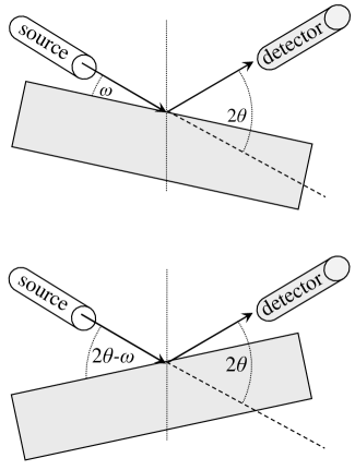
Figure 4: Geometrical arrangement of the diffuse $\omega$-scan scattering experiments with $2\theta$ being the angle of the incoming and outgoing waves, and $\omega$ being the angle of the incident wave and the surface of the stratified media. The lower part shows the setup obtained by a rotation by $\phi=2\left(\theta-\omega\right)$ around the axis being perpendicular to the scattering plane.

V Conclusion

As demonstrated in the general-level discussion, reciprocity is the property of a system – describing linear wavelike propagation – when it is connected with the adjoint system by an antiunitary operator. If the reciprocity property is fulfilled via such a reciprocity operator $K$ then a reciprocity theorem holds, which expresses the equality of any scattering amplitude $\langle\beta|T|\alpha\rangle$ to another scattering amplitude, namely, to $\langle K\alpha|T|K\beta\rangle$. This left-right interchange of incoming and outgoing states gives, in important experimental applications, that a scattering amplitude is related to another one where the source and the detector are interchanged.

Remarkably, reciprocity can hold for non-selfadjoint systems (systems with absorption), too. This immediately distinguishes reciprocity from time reversal invariance. Waves with spin/polarization degree of freedom demonstrate that reciprocity also differs from rotational invariance: Rotations are unable to map an incoming polarization degree of freedom to an outgoing one, nor an outgoing polarization to an incoming one. The above-presented calculations show in detail the relationship of reciprocity to time reversal as well as how rotation can be combined with reciprocity to obtain a version of the reciprocity theorem that is especially suitable for scattering experiments.

To find reciprocity operators for a given system is a delicate problem, which is solved here for an important class of physical situations, which cover applications in neutron and photon scattering on multilayer structures. Reciprocity violation is also quantified, and the results are illustrated and applied on examples, chosen from the area of Mössbauer scattering, where reciprocity is fulfilled for certain processes and is immensely violated for some others (scattering amplitudes differing remarkably).

The relationship established here to a recently developing area of mathematics is expected to give an impetus to finding reciprocity operators to more physical systems, resulting in valuable applications.