Halo Contraction Effect in Hydrodynamic Simulations of Galaxy Formation

Abstract

The condensation of gas and stars in the inner regions of dark matter halos leads to a more concentrated dark matter distribution. While this effect is based on simple gravitational physics, the question of its validity in hierarchical galaxy formation has led to an active debate in the literature. We use a collection of several state-of-the-art cosmological hydrodynamic simulations to study the halo contraction effect in systems ranging from dwarf galaxies to clusters of galaxies, at high and low redshift. The simulations are run by different groups with different codes and include hierarchical merging, gas cooling, star formation, and stellar feedback. We show that in all our cases the inner dark matter density increases relative to the matching simulation without baryon dissipation, at least by a factor of several. The strength of the contraction effect varies from system to system and cannot be reduced to a simple prescription. We present a revised analytical model that describes the contracted mass profile to an rms accuracy of about 10%. The model can be used to effectively bracket the response of the dark matter halo to baryon dissipation. The halo contraction effect is real and must be included in modeling of the mass distribution of galaxies and galaxy clusters.

1. Adiabatic Contraction in the Context of Hierarchical Galaxy Formation

Dissipationless cosmological simulations predict that virialized halos of dark matter are described by an approximately universal density profile (Dubinski & Carlberg, 1991; Navarro et al., 1997, 2010; Moore et al., 1998). Although non-baryonic dark matter exceeds normal baryonic matter by a factor of $\Omega_{\rm dm}/\Omega_{\rm b}\approx 5$ on average in the universe, the gravitational field in the central regions of galaxies can be dominated by stars and gas. In the hierarchical galaxy formation picture, cosmic gas dissipates its thermal energy, condenses towards the halo center, and forms stars. In the process, dark matter particles are pulled inward and increase their central density.

The response of dark matter to baryonic infall has traditionally been calculated using the model of adiabatic contraction (Eggen et al., 1962; Zeldovich et al., 1980; Barnes & White, 1984). The present form of the standard adiabatic contraction (SAC) model was introduced by Blumenthal et al. (1986) and Ryden & Gunn (1987). This model assumes that a spherically symmetric halo can be thought of as a sequence of concentric shells, made of particles on circular orbits, which homologously contract while conserving the angular momentum. With these assumptions, the final location $r_{f}$ of the shell enclosing mass $M_{\rm dm}(r)$, which was at radius $r$ before the contraction, can be calculated by knowing only the initial ($M_{{\rm b},i}$) and final ($M_{{\rm b},f}$) baryon mass profile:

$$\left[M_{\rm dm}(r)+M_{{\rm b},i}(r)\right]r=\left[M_{\rm dm}(r)+M_{{\rm b},f}(r_{f})\right]r_{f}.$$ (1)

Since the baryon mass typically increases at the inner radii as a result of dissipation ($M_{{\rm b},f}(r)>M_{{\rm b},i}(r)$), the final radius of the shell is smaller than the initial radius, $r_{f}<r$. That is, the halo contracts.

The effect of contraction of the dark matter distribution is important for many galactic studies: for modeling the mass profiles of galaxies and clusters of galaxies, for studying star formation feedback on the galactic structure, for abundance matching of galaxies and dark matter halos, for predicting possible signatures of dark matter annihilation, and others. This importance has led to a lively debate in the recent literature, both theoretical and observational, on the validity of the effect (we discuss it in more detail in Section 2). Hierarchical galaxy formation is considerably more complex than the simple picture of quiescent cooling in a static spherical halo. Every halo is assembled via a series of mergers of smaller units, with the cooling of gas and contraction of dark matter occurring separately in each progenitor. Some objects may undergo dissipationless merging after the gas is exhausted or the cooling time becomes too long. Any of these effects may invalidate the assumptions of the SAC model and possibly its prediction of halo contraction.

The only way to validate halo contraction is by investigating cosmological hydrodynamic simulations that self-consistently model as many of these complex processes as possible: gas dissipation, star formation, and its feedback. In Gnedin et al. (2004), we tested the SAC model using a suite of such simulations of the formation of one Milky Way-sized galaxy and eight clusters of galaxies, performed with the Adaptive Refinement Tree (ART) code. The comparison of the matching pairs of simulations with and without gas dissipation showed that the halos always contracted. However, the effect was weaker than that predicted by the SAC model. We developed a modified adiabatic contraction (MAC) model based on the modified invariant, $M(\bar{r})r$, where $\bar{r}$ is the orbit-averaged radius for particles currently located at radius $r$:

$$\left[M_{\rm dm}(\bar{r})+M_{{\rm b},i}(\bar{r})\right]r=\left[M_{\rm dm}(\bar{r})+M_{{\rm b},f}(\bar{r_{f}})\right]r_{f}.$$ (2)

Although this combination is not strictly conserved during galaxy formation, it is a simple correction that most accurately predicts the dark matter profiles in the simulations. Using the mass within the average radius approximately accounts for eccentricity of particle orbits in a cosmologically-assembled halo. Averaging over particle orbits in radial bins, we found a mean relation between $\bar{r}$ and $r$ in the range $10^{-3}\lesssim r/r_{\rm vir}\lesssim 1$:

$${\bar{r}\over r_{\rm vir}}=A\left({r\over r_{\rm vir}}\right)^{w},$$ (3)

where $r_{\rm vir}$ is the virial radius. This power-law dependence reflects typical energy and eccentricity distributions of particles in cold dark matter halos in the dissipationless simulations. The parameters $A$ and $w$ varied from halo to halo and from epoch to epoch. For the systems at hand we found the mean values $A\approx 0.85$ and $w\approx 0.8$, which we used as fiducial parameters of the model. We showed that the MAC model predicts the halo mass profile to 10%-20% accuracy.

Since 2004, several numerical and observational studies have evaluated the accuracy of the MAC model. We discuss these studies in Section 2. In particular, Gustafsson et al. (2006) found different amounts of contraction in their four simulated halos and suggested that different combinations of the model parameters may best fit individual profiles. Following the idea that the MAC model can be directly tested, in this paper we assemble a large collection of hydrodynamic simulations, of different systems run with different codes, to study the systematics of the contraction effect. We consider the effect of baryons only on the spherically-averaged radial halo distribution, although the halo shape is also affected (e.g., Kazantzidis et al., 2004; Abadi et al., 2010; Zemp et al., 2011).

2. Debate in the Literature

2.1. Theoretical Studies

Early controlled simulations confirmed the halo contraction effect (Sellwood & McGaugh, 2005; Choi et al., 2006; Colín et al., 2006).

Recently, Duffy et al. (2010) considered 67 galactic and galaxy group halos in three cosmological simulations with different feedback prescription with the Smooth Particle Hydrodynamics (SPH) code Gadget. They found the contraction effect in all cases, but each with a different amount of contraction. Similarly to Gustafsson et al. (2006), they explored the best-fit distribution of parameters $(A,w)$ and found them to be in the range $0.2-0.4$ at $z=0$. These parameter values may have been systematically lowered by the details of the fitting.

Abadi et al. (2010) studied 13 galaxy-sized halos simulated with the SPH code GASOLINE. The simulations included radiative cooling of cosmic gas above $10^{4}$ K but no cooling below $10^{4}$ K and no star formation. They found that in each case the halo contracted but by a smaller amount than predicted by either SAC or MAC model. However, the weaker contraction may be an artifact of the assumed gas physics, because their Figure 8 shows that the earlier simulations by the same authors (Abadi et al., 2003; Meza et al., 2003), which included star formation and feedback, agree much better with the MAC model.

Pedrosa et al. (2009, 2010) and Tissera et al. (2010) studied 6 halos in high-resolution SPH simulations with Gadget, with different prescriptions for star formation and feedback. They found halo contraction in all cases but again weaker than predicted by either SAC or MAC model. They suggest that the dynamical formation history may affect the amount of contraction in each individual halo.

In contrast to these studies, in a simulation of 3 galaxies with Gadget, Johansson et al. (2009) found that the dark matter mass contained with a fixed radius of 2 kpc increased at high redshift, reached a peak at $z\approx 3$, and then declined continuously to $z=0$. The central density decreased by up to a factor of two between $z=3$ and $z=0$, reaching the same value as in a matching dissipationless simulation and thus effectively canceling the contraction. Johansson et al. (2009) attribute the reduction of the dark matter density to gravitational heating by infalling dense stellar clumps. In their run most of the baryons in the halo were converted into stars at high redshift (stellar mass is 13% of the virial mass), creating massive stellar satellites, which may be too effective at pushing out dark matter. The evolution of the central density may also be affected by a spurious numerical effect due to two-body scattering of massive particles. This scattering would alter the profile on the two-body relaxation time, which at 2 kpc is about 9 Gyr in their highest-resolution run, and is shorter in other runs.

The SPH simulation of a large galaxy by Romano-Díaz et al. (2008) with constrained, rather than cosmological, initial conditions yielded an even more unexpected result. While they found the steepening of the dark matter profile at high redshift, the profile subsequently flattened to a constant-density core within the inner 3 kpc by $z=0$, reversing a contraction into an expansion. Such flattening is likely to be a numerical relaxation effect. Based on the information in their paper, we estimate that there are about 9000 particles within 3 kpc, which have a two-body relaxation time of about 14 Gyr. Thus the interaction of these particles can alter the true profile within the age of the universe.

Two new GASOLINE simulations, one for a dwarf galaxy (Governato et al., 2010) and one for a Milky Way-sized galaxy (Guedes et al., 2011), reach different conclusions on halo contraction. In the first case the central dark matter density is reduced, while in the second it is enhanced. Both simulations use the same strong blastwave feedback, which suppresses gas cooling around the star-forming region for several Myr and creates powerful outflows that remove a significant fraction of baryons from the halo (70% in the first run and 30% in the second run). The difference can be traced to a higher density threshold for star formation in the Governato et al. (2010) simulation, which means the supernova energy release is more concentrated and creates rapid potential fluctuations near the center. As Pontzen & Governato (2011) emphasize, the decrease of the inner dark matter density is achieved by repeated fluctuations following bursts of star formation, because a single outflow event cannot cause a significant change (e.g., Gnedin & Zhao, 2002). However, note that the Governato et al. (2010) result depends directly on the adopted parameters (their lower-threshold version in Governato et al. 2007 showed halo contraction instead of expansion) and thus it is one of many possible outcomes.

Overall, cosmological simulations performed by different authors with very different codes and physics input agree that the contraction effect is present, but at a weaker level than suggested by the SAC model and with a significant variation from system to system.

2.2. Observational Studies

Observational studies have generally provided evidence for halo contraction. Schulz et al. (2010) studied the mass distribution of a stacked sample of 75,000 elliptical galaxies from the Sloan Digital Sky Survey, combining weak lensing analysis in the outer regions of the halo with measurements of the stellar velocity dispersion in the inner regions. They found that halo contraction is required to explain the large and significant mass excess over the dissipationless NFW profile, in all luminosity bins. The MAC model gave excellent predictions to the data, while the SAC model overestimated the excess. An alternative explanation of the observed mass excess, by changing the stellar mass-to-light ratio, would require doubling the stellar mass relative to the Kroupa IMF.

Auger et al. (2010) studied the mass distribution of 53 early-type galaxies from the Sloan Lens ACS Survey, using a combination of stellar velocity dispersion measurements, strong lensing, and weak lensing. They found that the data favor a heavy stellar IMF and that halo contraction predicted by the MAC model improves the fit relative to the SAC model or to the case without halo contraction.

Minor & Kaplinghat (2008) investigated the effect of halo contraction on the statistics of strong gravitational lensing. They find that the contraction effect enhances the total lensing probability (similarly found by Rozo et al. 2008) and increases the ratio of double images relative to quad images and lensing cusps. In particular, without contraction naked cusp configurations would become dominant at angular separation as small as 2.5″, which is inconsistent with the data.

While early X-ray studies of the mass distribution in galaxy clusters (e.g., Zappacosta et al., 2006) disfavored halo contraction, Démoclès et al. (2010) studied the mass distribution in fossil galaxy groups (otherwise known as “X-Ray Overluminous Elliptical Galaxies”, see Vikhlinin et al. 1999) and found that halo contraction slightly improves the model fit.

Seigar et al. (2008) studied the mass distribution in the M31 galaxy and found that halo contraction is required to fit the inner regions. Without contraction, they cannot find any set of halo parameters that would reproduce the peak of the optical rotation curve at 10 kpc from the center, even with a very large halo mass. In fact, the best fit requires the SAC model, while the fiducial MAC model would need an unreasonably large concentration parameter of the dark matter halo.

Napolitano et al. (2011) derived the mass profile of a giant elliptical galaxy M84 using radial velocity measurements of planetary nebulae and field stars. The inclusion of the halo contraction effect, as parametrized by the MAC model, has allowed to derive the best-fit parameters of the dark halo to be in excellent agreement with the predictions of cosmological simulations. It is the first time that such agreement was achieved with the planetary nebulae kinematics.

Dutton et al. (2007, 2011) constructed semi-analytical models that simultaneously fit the luminosity function of galaxies and the Tully-Fisher/Faber-Jackson scaling relations. They found a preference for halo contraction for early-type galaxies, but a need for the opposite (halo expansion) for late-type galaxies. This conclusion is subject to additional uncertainty in the stellar mass-to-light ratio or the stellar IMF.

Benson & Bower (2010) investigated extensive observational data (galaxy sizes, clustering, luminosity function, mass-metallicity relation, Tully-Fisher relation, cosmic star formation history) using an improved version of the semi-analytical code galform and a flexible prescription for halo contraction using the MAC model. Their best-fit model required strong contraction ($A=0.74$, $w=0.92$; see also their Figure 7). Overall, they found a range of MAC model parameters ($A=0.74-0.96$, $w=0.81-0.99$) matching the multiple data constraints.

3. What controls the amount of contraction?

Gnedin et al. (2004) suggested that the eccentricity of dark matter particle orbits may be responsible for the weaker contraction effect seen in the simulations, relative to the SAC model. During the process of baryon condensation particle orbits can further deform, although Debattista et al. (2008) find that this effect is almost completely reversible if the baryons are subsequently removed (for example, by strong stellar feedback). In addition, during violent changes of the gravitational potential, such as those during galaxy mergers or interactions, the orbital structure may differ from that in a dynamical equilibrium. Then the orbital action variables are not strictly conserved and a first-principles calculation of the contraction effect becomes even more difficult.

Our original power-law approximation for the average orbit radius $\bar{r}$ was derived as an average of several dissipationless simulations of galaxy-sized and cluster-sized halos. Hydrodynamic SPH simulations of Gustafsson et al. (2006) confirmed that Equation (3) is an excellent fit in the inner parts of halos. They fit each of their four simulated halos with an independent set of the parameters $A$ and $w$, and found them to lie in the range $A=0.74-0.83$, $w=0.69-0.81$. The values of the parameters in our MAC model are consistent with these ranges. However, the results of Gustafsson et al. (2006) indicated that each simulated system may have somewhat differing amounts of contraction.

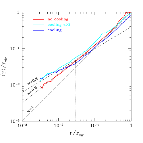
Figure 1.— Average orbital radius vs. instantaneous radius of dark matter particles in a dissipationless and two dissipational runs of a cluster-sized halo at $z=0$. This halo is described in the second line in Table 1 and in Section 4.1. The size of the smallest resolution element is $\Delta=1.7\times 10^{-3}\,r_{\rm vir}$. In one simulation the gas cooling is suppressed at $z<2$. Dotted and dashed lines show the slopes in the inner halo, with $w=0.8$ and $w=0.6$, respectively. Long-dashed line shows the relation in the SAC model. Vertical dotted line marks new pivot radius $r_{0}$ in Equation 4. Vertical arrow illustrates an adjustment by factor of 1.6 required for new normalization $A_{0}$.

To better understand the orbital dependence, we investigated the $\bar{r}-r$ relation in our hydrodynamic run for “Cluster 6” (shown in Figures 1 and 2 in Gnedin et al. 2004). We computed a proxy for the average orbital radius, $\bar{r}\approx\langle r\rangle$, by integrating orbits in a static NFW potential normalized to the maximum circular velocity $V_{\rm max}$ measured in the simulation. Note that while the normalization of the profile correctly takes into account the baryon condensation, the shape of the potential may deviate from the NFW form in the dissipative runs. Figure 1 shows that while the dissipationless run is well characterized by our fiducial slope $w\approx 0.8$, the run with cooling and star formation shows a more complex relation, with departures from a single power law. The outer regions, between $0.1r_{\rm vir}$ and $r_{\rm vir}$, have a steep slope $w\approx 1$ (the virial radius is calculated at the overdensity of 180 with respect to the mean cosmic density). The inner regions have much flatter slope, $w\approx 0.5$, similar to the values reported by Gustafsson et al. (2006). In these inner regions, $r<0.03r_{\rm vir}$, the contribution of baryons to the mass profile becomes significant and the contraction effect should be most important. Thus for the purpose of calibrating the contraction model, we can restrict the fit of a power-law slope just to the inner regions.

Interestingly, in the run in which cooling and star formation were turned off at $z<2$, the $\bar{r}-r$ relation in the outer halo is closer to that in the dissipationless run than in the full dissipative run. In the inner halo, the slope is again flatter, $w\approx 0.6$. In this run the stellar fraction within the virial radius is half of that in the full run and is closer to the observed fraction in galaxy clusters. After the cooling was stopped, the gravitational potential in the inner halo probably did not evolve and allowed the particle orbits to come to dynamical equilibrium. Therefore, the contraction effect may depend not only on the final amount of baryon condensation but also on the duration of this process.

Since the $\bar{r}-r$ relation evolves during the process of dissipation, a MAC model with fixed parameters $A$ and $w$ cannot accurately describe the contraction effect. Instead, following Gustafsson et al. (2006), we can search for the best-fitting values of the model parameters for each simulated halo and then analyze their distribution.

Figure 1 also shows that if we are to vary $w$, the normalization $A$ would have to vary correspondingly because Equation (3) is anchored at $r_{\rm vir}$, far from the region of interest in the inner halo. We can reduce this correlated variation of $A$ by shifting the pivot of the $\bar{r}-r$ relation to some inner radius, $r_{0}$. The correlation between $w$ and $A$, which we derive for the simulations described below, is minimized for $r_{0}\approx 0.03\,r_{\rm vir}$. Therefore, we redefine the relation of the MAC model as

$${\bar{r}\over r_{0}}=A_{0}\left({r\over r_{0}}\right)^{w}.$$ (4)

We use the subscript “0” to differentiate this normalization parameter $A_{0}$ from its original version in Gnedin et al. (2004) defined by Equation (3). We fix the pivot at $r_{0}=0.03\,r_{\rm vir}$ in all discussion that follows. Only the normalization $A_{0}$ is affected by this shift of the pivot point from $r_{\rm vir}$ to $r_{0}$, the slope $w$ remains invariant. The SAC model is still characterized by $A_{0}=w=1$.

3.1. The role of model parameters

To understand the effect of varying the parameters $A$ and $w$ on the amount of contraction, consider the inner regions of a halo. The contraction factor $y\equiv r_{f}/r$ obeys Equation (2), which after dividing both sides by $M_{i}(\bar{r})r_{f}$ becomes

$${1\over y}=1-f_{b}+{M_{b}(\overline{ry})\over M_{i}(\bar{r})},$$ (5)

where $f_{b}$ is the baryon fraction within the virial radius of the halo of interest. The average cosmic baryon fraction is $f_{b}\approx 0.17$, but a given halo may have a different baryon fraction. Here $M_{i}(r)\equiv M_{{\rm dm},i}(r)+M_{{\rm b},i}(r)$ is the total initial mass, the sum of dark matter and baryons. Typically, before contraction the dark matter profile shadows the total mass distribution, $M_{{\rm dm},i}(r)\approx(1-f_{b})\,M_{i}(r)$.

In the inner halo described by an NFW profile with the scale radius $r_{s}$, the initial enclosed mass is $M_{i}(r)\propto r^{2}$ at $r\ll r_{s}$. In this region, we can define the average logarithmic slope of the final baryon density profile: $\rho_{b}\propto r^{-\nu}$, which lies in the range $1<\nu<3$ ($\nu\approx 2$ is typical; Koopmans et al. 2009). Then the final baryon mass profile $M_{b}(r)\propto r^{3-\nu}$, and Equation (5) becomes

$${1\over y}=1-f_{b}+{M_{b}(\bar{r})\over M_{i}(\bar{r})}\;y^{w(3-\nu)}.$$ (6)

The enhancement factor of the dark matter mass profile is given by Equation (A11) of Gnedin et al. (2004) and is most easily evaluated at the contracted radius $r_{f}=ry(r)$:

$$F_{M}(ry)\equiv{M_{{\rm dm},f}(ry)\over M_{{\rm dm},i}(ry)}={M_{{\rm dm},i}(r)\over M_{{\rm dm},i}(ry)}\approx{1\over y(r)^{2}}.$$ (7)

The last approximation is valid only in the inner region where $M_{i}(r)\propto r^{2}$. For arbitrary $\nu$ and $w$, Equation (6) is transcendental and must be solved numerically. However, a good second-order approximation is described in Appendix.

To make concrete calculations using Equations (6) and (7), we must specify the ratio of the final baryon enclosed mass to the initial total enclosed mass. Let $r_{e}$ be the radius where the final baryon mass equals the initial dark matter mass: $M_{b}(r_{e})\equiv M_{{\rm dm},i}(r_{e})$. For the Milky Way galaxy, this radius is about 10 kpc, and thus a good choice is $r_{e}\approx 0.05\,r_{\rm vir}$. It then follows that $M_{b}(\bar{r})/M_{i}(\bar{r})=(1-f_{b})\,(\bar{r}/r_{e})^{1-\nu}$.

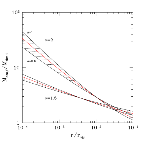
Figure 2.— Enhancement of the enclosed dark matter mass given by Equation (7) for the inner halo. The top shaded region corresponds to the baryon density slope $\nu=2$, the bottom region to $\nu=1.5$. Each region is bounded by the lines of the contraction models with the MAC parameter $w=1$ (upper) and $w=0.6$ (lower). The middle line is for $w=0.8$. The parameter $A_{0}$ is set to 1.6 in all cases. The baryon mass profile is normalized to be equal to the initial dark matter mass at $r_{e}=0.05\,r_{\rm vir}$.

Figure 2 shows the mass enhancement factor using the numerical solutions of Equation (6) for two representative values of $\nu=2$ and $\nu=1.5$. In the inner halo, the stronger baryon dissipation ($\nu=2$ vs. $\nu=1.5$) leads to the stronger contraction of dark matter. Larger value of $w$ and smaller value of $A_{0}$ indicate stronger contraction effect at small radii. However, there is a cross-over point for the lines of different $w$, and the trend is reversed at the intermediate radii ($0.01-0.1\,r_{\rm vir}$). While both $A_{0}$ and $w$ determine the normalization of $F_{M}$, the parameter $w$ determines also the increase of the amount of contraction with radius.

Table 1Simulations and MAC model parameters

System	$M_{\rm vir}$ ($M_{\sun}$)	$A_{0}$	$w$	rms	$w^{a}$	rmsa	Ref
Cluster	$3.4\times 10^{14}$	1.83	1.33	0.037	1.29	0.060	G04
Cluster	$3.7\times 10^{14}$	1.74	0.51	0.028	0.50	0.045	G04
Cluster	$3.8\times 10^{14}$	1.54	0.74	0.015	0.76	0.022	G04
Cluster	$2.1\times 10^{14}$	2.30	1.48	0.051	1.57	0.140	G04
Cluster	$1.4\times 10^{14}$	1.78	0.71	0.009	0.79	0.053	G04
Cluster	$2.0\times 10^{14}$	1.28	0.55	0.027	0.37	0.100	G04
Cluster	$1.9\times 10^{14}$	1.54	1.03	0.007	1.02	0.016	G04
Cluster	$1.2\times 10^{14}$	1.24	0.87	0.013	0.61	0.232	G04
Group	$8.6\times 10^{13}$	1.42	0.67	0.009	0.55	0.032	N06
Group	$4.0\times 10^{13}$	1.30	1.06	0.005	0.81	0.030	N06
Group	$7.1\times 10^{13}$	1.47	0.91	0.011	0.82	0.024	N06
Group	$1.1\times 10^{14}$	1.43	1.11	0.023	0.98	0.036	N06
Group	$5.3\times 10^{13}$	1.14	1.22	0.035	0.84	0.067	N06
Group	$7.3\times 10^{13}$	2.06	0.91	0.012	1.24	0.078	N06
Group	$9.8\times 10^{13}$	1.59	0.85	0.017	0.84	0.057	N06
Group	$7.6\times 10^{13}$	1.41	0.69	0.009	0.55	0.031	N06
Group	$6.1\times 10^{13}$	0.75	1.28	0.008	0.59	0.135	N06
Group	$2.1\times 10^{13}$	1.12	1.29	0.020	0.90	0.048	N06
Group	$1.9\times 10^{13}$	1.87	0.62	0.010	0.77	0.017	N06
Group	$1.2\times 10^{14}$	1.61	0.86	0.027	0.86	0.027	N06
Galaxy	$5.5\times 10^{11}$	2.65	1.38	0.009	0.85	0.107	G10
Galaxy	$7.5\times 10^{11}$	1.79	1.20	0.014	1.07	0.034	G10
Galaxy	$2.8\times 10^{11}$	1.21	0.67	0.016	0.91	0.068	G10
Galaxy $z=1$	$8.4\times 10^{11}$	2.07	0.64	0.021	0.99	0.081	C09
Galaxy $z=1$	$4.8\times 10^{10}$	2.92	0.85	0.023	1.31	0.266	C09
Galaxy $z=3$	$3.4\times 10^{11}$	1.32	1.26	0.103	1.26	0.144	L08

Note: ^a for fixed $A_{0}=1.6$.
References: G04 = Gnedin et al. (2004), N06 = Nagai (2006), G10 = Gottloeber et al. (2010), C09 = Ceverino & Klypin (2009), L08 = Levine et al. (2008).

4. Cosmological hydrodynamic simulations

In this section we describe the simulations of galaxy formation that we use to test the MAC model. We tried to collect as diverse samples of simulations and codes as possible and to analyze them at $z=0$, so as to evaluate the applicability of the model to observations. We also consider a few interesting cases at $z=1$ and $z=3$.

We fit both the original set of parameters $A$ and $w$ from Equation (3) and the modified set $A_{0}$ and $w$ from Equation (4). The latter set for each system is summarized in Table 1.

To derive the best-fit parameters we minimize the difference between the enclosed mass in a radial bin in the dissipative simulation, $M_{{\rm sim}}$, and the corresponding mass predicted by the MAC model, $M_{{\rm mod}}$. For convenience, we define the following dimensionless difference in radial bin $i$:

$$z_{i}\equiv{M_{{\rm mod},i}\over M_{{\rm sim},i}}-1.$$ (8)

The “correct” mass profile in the dissipative simulation is not known infinitely precisely, and therefore the model should match it only within certain fidelity, $\sigma_{i}$. The best-fit values of the parameters are obtained by minimizing the $\chi^{2}$ function

$$\chi^{2}=\sum_{i}{z_{i}^{2}\over\sigma_{i}^{2}}.$$ (9)

We include two sources of uncertainty in $\sigma_{i}$. The first is a simple Poisson counting error, which we take to be the square root of the number of particles in the bin, $N_{i}^{-1/2}$. The other is systematic uncertainty in the spherical mass profile, which can arise from a number of effects such as a triaxiality of the halo, an ongoing merger event, or a small mismatch in the output timing between the dissipational and dissipationless simulations. In such cases the deviation in some radial bins between the predicted model profile from the simulated profile may be large, even if the bin contains thousands of particles. We model this uncertainty as a constant error in each bin, $\sigma_{\mathrm{sys}}$, that puts an upper limit on the value of $\chi^{2}$. This allows us to obtain controlled, even if only relative, estimates of the confidence intervals of the model parameters. The value of $\sigma_{\mathrm{sys}}$ is set such that for the SAC model ($A_{0}=w=1$) it would result in a specified value of $\chi^{2}$ per degree of freedom (equal to $N_{\mathrm{sys}}$):

$$\sigma_{\mathrm{sys}}^{2}\equiv{1\over N_{\mathrm{sys}}}{1\over N_{b}-2}\sum_{i}z_{i}^{2},$$ (10)

where $N_{b}$ is the number of bins, and the number of degrees of freedom is $N_{b}-2$ when we are fitting two model parameters. Once we set $\sigma_{\mathrm{sys}}$, it is then kept fixed as we search for the best-fitting parameters $A$ and $w$.

We take a large enough value, $N_{\mathrm{sys}}=100$, such that it would not alter fitting in the bins with fewer than 100 particles, while avoiding large deviations in the more populous bins. We have verified that choosing any value in the range $10<N_{\mathrm{sys}}<1000$ results in similar model parameters. The total error in bin $i$ is

$$\sigma_{i}^{2}={1\over N_{i}}+\sigma_{\mathrm{sys}}^{2}.$$ (11)

As an alternative to minimizing the $\chi^{2}$ function, we have also tested a robust estimator $\sum|z_{i}|/\sigma_{i}$, which is not sensitive to distant outliers. With both methods we obtained essentially the same best-fit parameters for our simulations.

In order to make the most accurate fit in the region where the contraction effect is important, we restrict the radial bins included in the fitting to $r<0.1\,r_{\rm vir}$. We allow the parameters to vary in the range $0<A_{0}\leq 3$, $0<w\leq 2$. Even larger values would yield models degenerate with those in the chosen range, as it will become clear later in Figure 6.

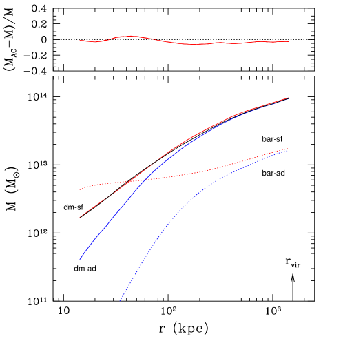
Figure 3.— Contraction of the dark matter profile in a simulated group of galaxies at $z=0$, from Nagai (2006). Solid lines show the enclosed dark matter mass profile, in the non-radiative (ad) run and star formation (sf) run. Dotted lines show the corresponding baryon mass profiles. Black solid line is the best fit of the MAC model, with parameters $A_{0}=1.61$, $w=0.86$. Top panel shows the mass residuals for the MAC model with freely adjustable $A_{0}$ (solid) and the MAC model with fixed $A_{0}=1.6$ (dashed). In this plot the two lines almost coincide.

4.1. Clusters and groups of galaxies

The first sample consists of the simulations of 8 galaxy cluster halos described in Gnedin et al. (2004) and additional 12 galaxy group halos by Nagai (2006) with the same setup. These are high-resolution cosmological simulations in the $\Lambda$CDM model ($\Omega_{\rm m}=0.3$, $\Omega_{\Lambda}=0.7$, $\Omega_{\rm b}=0.043$, $h=0.7$, $\sigma_{8}=0.9$) performed with the ART code (Kravtsov, 1999; Kravtsov, Klypin, & Hoffman, 2002). The simulations have a peak spatial resolution $\Delta=3.5$ kpc and dark matter particle mass of $3.9\times 10^{8}\,M_{\sun}$. The virial mass of the systems ranges from $2\times 10^{13}\,M_{\sun}$ to $4\times 10^{14}\,M_{\sun}$. Star formation is implemented using the standard Kennicutt’s law and is allowed to proceed in regions with temperature $T<10^{4}$ K and gas density $n_{g}>0.1\ \rm cm^{-3}$. We truncate the inner profiles at $4\Delta$ to ensure that the gravitational dynamics is calculated correctly in the studied region.

Figure 3 shows the mass profiles for one of the groups. The dark matter mass is significantly enhanced in the star formation run relative to the non-radiative run, by a factor of 4 at the innermost resolved radius. The baryons strongly dominate the total mass at that point. The MAC model provides an excellent fit to the contracted dark matter profile, with the parameters ($A_{0}=1.61$, $w=0.86$) close to the fiducial values. The maximum deviation of the mass profile predicted by the MAC model is 6%, and the rms deviation over all bins at radii $r<0.1\,r_{\rm vir}$ is 3%. We similarly analyzed the other eleven groups and present their best-fit parameters in the discussion of Figure 6.

4.2. Individual Galaxies

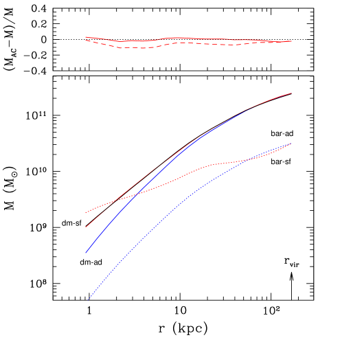
Figure 4.— Contraction of the dark matter profile in a simulated galaxy at $z=0$, from Gottloeber et al. (2010). Line notation is the same as in Figure 3. Black solid line is the best-fit MAC model with $A_{0}=1.79$, $w=1.2$. Dashed line in top panel shows the MAC model prediction with fixed $A_{0}=1.6$, and best-fitting $w=1.07$.

We consider the simulation of three Milky Way-sized galaxies by the CLUES project (http://www.clues-project.org; Gottloeber et al., 2010; Knebe et al., 2010). The simulation is run using the SPH code Gadget-2. This code includes standard radiative cooling, star formation, and supernova feedback. The force softening length $\epsilon=0.14$ kpc. The halos were selected from a large box and resimulated with the effective mass resolution of $4096^{3}$ dark matter particles. In the highest-resolution halos the particle mass is $3.5\times 10^{5}\,M_{\sun}$. The virial masses of the three halos at $z=0$ are $(3-8)\times 10^{11}\ M_{\sun}$. The inner truncation radius is set by the condition that the local two-body relaxation time exceeds the age of the universe.

Figure 4 shows the profile of the most massive of the three galaxies. The dark matter mass is enhanced by an order of magnitude at the innermost radius. The MAC model with parameters ($A_{0}=1.79$, $w=1.2$) predicts the dark matter profile to better than 4% accuracy in any bin, with the rms deviation of only 1.4%.

We consider also the simulations of a Milky Way-sized galaxy and a dwarf galaxy at $z=1$ by Ceverino & Klypin (2009). These simulations are run with the ART code with a very different prescription for stellar feedback than in Nagai (2006). The large galaxy mass is $8\times 10^{11}\,M_{\sun}$, the dwarf galaxy mass is $5\times 10^{10}\,M_{\sun}$, both at $z=1$. The dark matter particle mass is $7.5\times 10^{5}\,M_{\sun}$ and the peak spatial resolution is 100 comoving pc for the larger galaxy. For the smaller galaxy, the dark matter particle mass is $9.4\times 10^{4}\,M_{\sun}$ and the peak resolution is 50 comoving pc. Compared to the non-radiative runs, the dark matter mass is enhanced by a factor of 8 for the larger galaxy and by a factor of 5 for the smaller galaxy, at the innermost radius. The MAC model (with parameters $A_{0}=2.07$, $w=0.64$ and $A_{0}=2.92$, $w=0.85$, respectively) predicts the dark matter profile to better than 9% accuracy, with the rms deviation of about 2%.

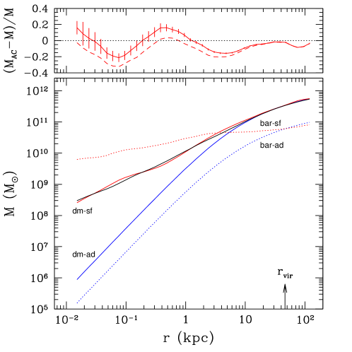
Figure 5.— Contraction of the dark matter profile in a simulated galaxy at $z=3$, from Levine et al. (2008). Line notation is the same as in Figure 3. Black solid line is the best-fit MAC model with $A_{0}=1.32$, $w=1.26$. Vertical bars on the MAC model in the top panel indicate the Poisson uncertainty of the mass profile derived in the simulation. Dashed line in top panel shows the MAC model prediction with fixed $A_{0}=1.6$, and best-fitting $w=1.26$.

4.3. Galaxy Center

Finally, we consider the resimulation of the galaxy run reported in Gnedin et al. (2004) that zooms into the innermost region of the galaxy at $z=3$ (Levine et al., 2008). This simulation follows the early evolution of a galaxy that becomes a Milky Way-sized object at $z=0$. The DM particle mass is $1.3\times 10^{6}\,M_{\sun}$ and the peak force resolution at $z=3$ is 0.064 kpc for the gas and 0.1 kpc for the dark matter, a very small scale for cosmological simulations. We truncate the inner profile such that the innermost bin contains at least 200 dark matter particles.

Figure 5 shows that the MAC model is able to describe even this case, with the rms deviation of 10%. This case is extreme because the baryons dominate the dark matter by two orders of magnitude at the innermost radius, and the dark matter mass is enhanced by a factor of 300 relative to the extrapolation of the dissipationless profile.

We also note that the stellar profile is contracted similarly to the dark mater profile, because gas accretion is faster than star formation.

5. Distribution of model parameters

All of the simulations considered here indicate some degree of enhancement of the dark matter profile. Not a single case indicates halo expansion rather than contraction. Figure 6 combines the resulting constraints on the parameters $A$ and $w$ of Equation (3). The models do not fill all the available parameter space, but instead concentrate in a fairly narrow region in which $A$ and $w$ are strongly correlated. The original MAC model suggested by Gnedin et al. (2004) falls right in the middle of the new distribution.

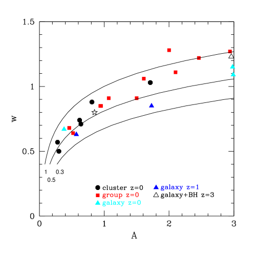
Figure 6.— Best-fitting parameters of the original MAC model (Equation 3) for all simulations discussed in this paper. Asterisk marks the fiducial parameters of the MAC model in Gnedin et al. (2004). Solid lines show the relation between $A$ and $w$ that gives the same amount of contraction (enhancement of dark matter mass) at $r=0.005\,r_{\rm vir}$, for the baryon profile with $\nu=2$ normalized to equal the initial dark matter mass at $r_{e}=0.05\,r_{\rm vir}$. The top line gives the same amount of contraction as the SAC model. The other two lines correspond to 50% and 30% of that amount.

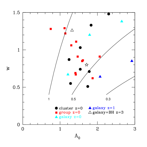
Figure 7.— Best-fitting parameters of the revised MAC model with $r_{0}=0.03\,r_{\rm vir}$ (Equation 4). Symbols and lines are as in Figure 6.

It is interesting to determine which combination of the parameters $A$ and $w$ yields the same amount of contraction. Given the radial dependence of the mass enhancement factor $F_{M}$ (Equation 7), the solution to this problem varies with radius. However, we can remove most of the radial dependence by defining the enhancement factor relative to the SAC model:

$$f_{M}\equiv{F_{M}(r|A,w)\over F_{M}(r|1,1)}$$ (12)

and evaluating it at some inner radius where the linear approximation for the contraction factor $y(r)$ is valid. We take $r=0.005\,r_{\rm vir}$, which corresponds to about 1 kpc for the Milky Way galaxy. The exact value of $r$ affects the resulting value of parameter $w$ (for a given $A$) only logarithmically, as long as $r\ll r_{e}$, which we take again to be $r_{e}=0.05\,r_{\rm vir}$.

Lines in Figure 6 show the relation between $A$ and $w$ corresponding to three values of $f_{M}$. All simulations but three fall below the level of contraction predicted by the SAC model. At the same time, no simulation falls below the level of $f_{M}=0.3$. Therefore, the MAC model is well constrained to be able to reliably predict the amount of dark matter in the inner regions of galaxies and clusters.

The isocontours of constant $f_{M}$ become even more horizontal at smaller $r$. This suggests that parameter $w$ may be more important than $A$ in describing the amount of contraction. It is also desirable to describe the strength of the contraction effect by only one parameter instead of two. The first step in this direction is to eliminate or reduce the apparent correlation between $A$ and $w$. To this aim, we calculated the best-fitting parameters of the revised model (Equation 4) and determined the pivot radius $r_{0}$ that minimizes the correlation. It is the value $r_{0}=0.03\,r_{\rm vir}$ quoted above. Figure 7 shows the new distribution of the resulting best-fit parameters $A_{0}$ and $w$. The values of $w$ are essentially unchanged, but the values of $A_{0}$ are more concentrated than the distribution of $A$ in Figure 6. The residual scatter of $A_{0}$ reflects intrinsic variation of the strength of halo contraction among different systems. The isocontours of constant $f_{M}$ also correspondingly change shape.

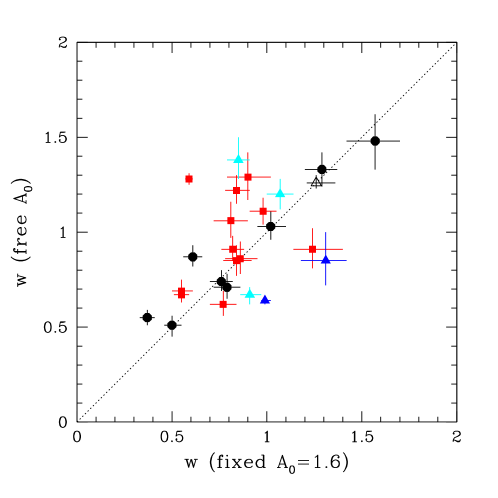
Figure 8.— Comparison of the best-fitting parameters $w$ obtained with variable $A_{0}$ with those obtained for fixed $A_{0}=1.6$. Sizes of the errorbars are relative.

The second step in simplifying the model prescription is fixing the parameter $A_{0}$. We take the average value $A_{0}\approx 1.6$ and redo all model fits allowing only for the variation of $w$. The best-fit values are listed in Table 1. Obviously, a one-parameter fit is less accurate than the two-parameter fit, but the rms error of mass is still typically below 10%. The one-parameter fits also do not introduce systematic shifts in the derived values of $w$, as shown in Figure 8. Thus, $w$ can serve as a convenient measure of the strength of halo contraction.

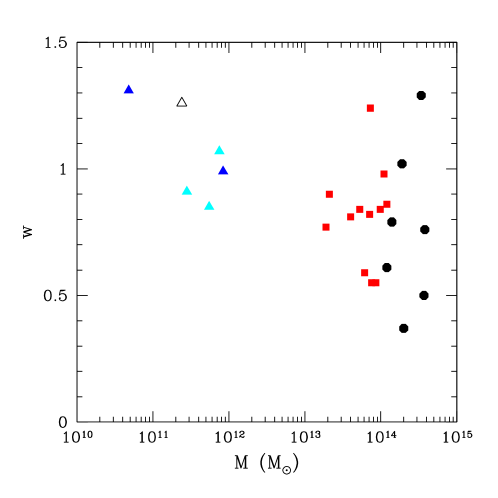
Figure 9.— Best-fitting parameter $w$ (for fixed $A_{0}=1.6$) vs. halo mass for all systems in our compilation.

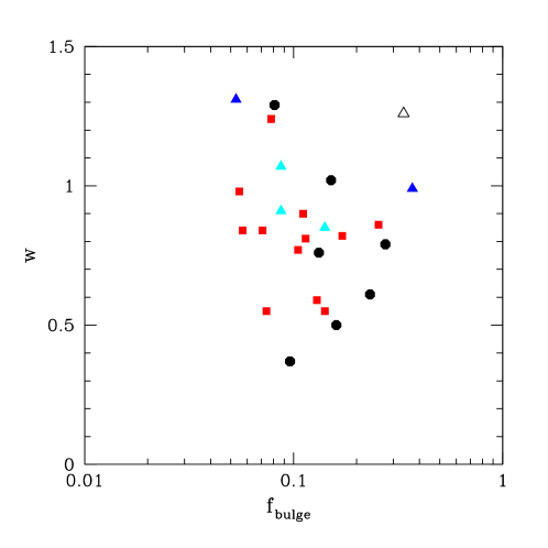
Figure 10.— Best-fitting parameter $w$ (for fixed $A_{0}=1.6$) vs. the bulge fraction, defined as the fraction of baryon mass contained within $0.01\,r_{\rm vir}$.

In practical application of the contraction model to observations or dissipationless simulations we wish to know the value of $w$ most appropriate to a given system. We considered several properties of the simulated halos but, unfortunately, we were unable to find significant correlation with $w$. For example, Figure 9 shows that $w$ is effectively independent of halo mass. Only the lower envelope of the distribution decreases with $M_{\rm vir}$.

We have looked for other potential correlations: with the ratio of final baryon mass to initial dark matter mass at the innermost resolved radius and at a fixed radius of $0.01\,r_{\rm vir}$, with the ratio of final dark matter to baryon mass at $0.01\,r_{\rm vir}$, and with the bulge fraction of galaxies. The latter is defined as the fraction of baryon mass contained within $0.01\,r_{\rm vir}$: $f_{\mathrm{bulge}}\equiv M_{*}(0.01\,r_{\rm vir})/M_{*}$. Figure 10 shows the scatter plot of $w$ with the bulge fraction, lacking any significant correlation.

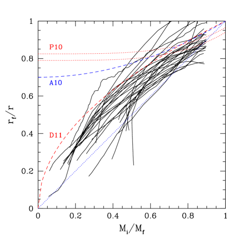
Figure 11.— Model-independent strength of the contraction effect. Solid lines are for all systems in our compilation. Dashed blue line is the relation suggested by Abadi et al. (2010), dotted lines are the relations suggested by Pedrosa et al. (2010), dashed red line is a relation of the type suggested by Dutton et al. (2011) but with $n=0.5$ instead of $n=-0.5$ (which would go off the scale of the plot).

6. Is halo contraction real?

The strength of the contraction effect can be assessed in a model-independent way, as suggested by Abadi et al. (2010). They expressed the ratio of the contracted to initial radius of spherical shells as a function of the ratio of initial to final total mass. In the SAC model this relation is expected to be unity, $r_{f}/r=M_{i}(r)/M_{f}(r_{f})$. For a weaker contraction effect, we expect $r_{f}/r>M_{i}/M_{f}$. Abadi et al. (2010) found that in their simulations the dark matter shells contract on the average as $r_{f}/r=1+0.3[(M_{i}/M_{f})^{2}-1]$. Pedrosa et al. (2010) did a similar analysis for their simulations but found different relations: $r_{f}/r=1+0.14[(M_{i}/M_{f})^{4}-1.25]$ for early-type galaxies, and $r_{f}/r=1+0.15[(M_{i}/M_{f})^{4}-1.4]$ for late-type galaxies.

Figure 11 shows the contraction factor for all of our simulations. The effect is clearly more significant than suggested by the above relations. In several cases, the contraction is even stronger at the innermost radii than that predicted by the SAC model, that is $r_{f}/r<M_{i}/M_{f}$. It can also be seen in Figure 7. Overall, there is no single relation for the contraction factor $r_{f}/r$. The scatter among different systems is intrinsic, similar to the scatter of model parameters $A$ and $w$.

Dutton et al. (2011) constructed semi-analytical models of galaxy populations using, in addition to the MAC model, an analytic prescription for either halo contraction or expansion of the form $r_{f}/r=(M_{i}/M_{f})^{n}$, with $n$ as a free parameter. Their preferred case is halo expansion with $n=-0.5$. None of our systems shows evidence for such expansion. If we were to use this parametrization to envelop the distribution of our simulations, then most of our results would lie within the range $0.6<n<1.2$. However, such parametrization has no physical basis and we do not recommend it.

Is the halo contraction effect real? Much of the apparent controversy in the literature on the validity of the contraction effect is due to the strict application of adiabatic invariants. In fact, most of the hydrodynamic cosmological simulations are in agreement that the effect is real and, at the same time, weaker than that expected in the Blumenthal et al. (1986) model. To avoid future controversy, we propose to abandon the term “adiabatic contraction” (reserving it only for the SAC model for historical reasons) and instead use the term “halo contraction”.

Note that all individual effects that were proposed to “reverse” contraction (such as the rapid supernova winds, cold accretion, galactic bars, inspiraling of dense baryonic clumps by dynamical friction, etc.) are already included in self-consistent cosmological simulations and differ only in the specific implementation (numerical resolution, star formation prescription, feedback model). Isolated investigations of these effects therefore do not invalidate the conclusions we derive from the ensemble of the simulations presented here. One should not also attribute halo contraction only to dissipative galaxy formation and contrast it with dissipationless accretion of satellites (e.g., Lackner & Ostriker, 2010) because both processes are taking place simultaneously. Hydrodynamic simulations are steadily improving in accuracy and will continue to include and evaluate new effects, such as the repeated potential fluctuations following bursts of star formation (Pontzen & Governato, 2011), mechanical and radiative feedback of active galactic nuclei, etc. Our ability to model halo contraction will continue to evolve along with our overall understanding of galaxy formation.

The MAC model does not presume a specific amount of contraction. It is a method for calculating the dynamical response of the dark matter halo to a given accumulated mass of baryons. The model is based on simple underlying physics and not just fitting the results of a particular simulation. The halo response depends directly on the change of the baryon profile relative to the dissipationless formation. As such, the response may be a halo expansion if more baryons are removed from the galaxy center than were there initially. For example, Sommer-Larsen & Limousin (2010) gradually reduced the stellar mass in their simulated galaxy cluster between $z=2$ and $z=0$, and found a much reduced contraction effect at the end, as would be expected if the removed stars did not form at all.

How should halo contraction be included in modeling of observed systems or in theoretical semi-analytical models based on dissipationless simulations? Direct parametrization of the form suggested by Abadi et al. (2010) can only be used when the final distribution of dark matter is known, that is, only for comparing results of hydrodynamic simulations with each other. When the distribution of dark matter needs to be predicted, the MAC model provides a reasonably accurate method and requires knowing only the final baryon profile. Unfortunately, the values of the model parameters have irreducible scatter and do not appear to correlate with any obvious property of the system of interest. Thus the model prediction carries some irreducible uncertainty. In practical application it suffices to account for this uncertainty by varying only one of the two parameters. We advocate the choice of $A_{0}$ and $w$ (Equation 4) instead of $A$ and $w$ (Equation 3) because the new parameters are effectively uncorrelated. For assessing the effect of halo contraction on a given system, we suggest fixing $A_{0}=1.6$ and varying $w$ in the range $0.6-1.3$. This prescription covers most of the parameter range seen in our simulations (Figure 7) while providing the estimate of the dark matter mass profile with rms accuracy of about 10% (Table 1).

What is the origin of the intrinsic scatter of the parameters $A_{0}$ and $w$, or of the contraction factor $r_{f}/r$? We can identify a number of processes in galaxy formation that could produce such scatter. For example, baryons in different galaxies condense at different epochs and have different angular momentum profiles, both of which affect the compactness of the final baryon distribution. In addition, galaxies experience different amounts of merger activity, which can change the morphology of baryon distribution and can gravitationally heat dark matter. Given these and other factors, it would be surprising if the intrinsic scatter did not exist. It is not known at the moment which of these effects are dominant. It would be useful to explore the origin of the intrinsic scatter in future studies.

7. Conclusions

We have evaluated the halo contraction effect using a large compilation of cosmological hydrodynamic simulations performed by different groups with different codes. In all the cases we considered, we find an increase of the dark matter density in inner regions of galaxies and clusters, relative to the matching dissipationless simulation. The halo contraction effect is real and must be included in the modeling of observations and in the semi-analytical theoretical modeling.

The contraction effect is weaker than predicted by the adiabatic contraction model of Blumenthal et al. (1986). However, depending on the system and the final baryon distribution, the inner dark matter density is still enhanced typically by a factor of several, and in extreme cases by two orders of magnitude.

The revised MAC model offers a convenient and accurate way to estimate the effect of halo contraction. The distribution of model parameters cannot be reduced to a single number, but their range is well constrained: $1<A_{0}<2.2$, $0.6<w<1.3$. We find that fixing the value of $A_{0}=1.6$ does not significantly degrade the accuracy of the predicted mass profile, relative to the two-parameter fit. We suggest varying $w$ in the range $0.6-1.3$ in order to bracket a possible response of the dark matter halo in a given system of interest.

The revised MAC model is encoded in the software package Contra, available for download at http://www.astro.lsa.umich.edu/$\sim$ognedin/contra.

Appendix A Analytical approximation for the contraction model

An approximate analytical solution of Equation (6) for the contraction factor $y\equiv r_{f}/r$ can be obtained as follows. At $r\ll r_{e}$, the ratio $M_{b}(\bar{r})/M_{i}(\bar{r})\gg 1$ and the term $(1-f_{b})$ can be neglected. The first-order approximation is therefore

$$y_{0}=\left[{M_{b}(\bar{r})\over M_{i}(\bar{r})}\right]^{-{1\over 1+w(3-\nu)}}.$$ (A1)

Then we can express the correct solution as $y=y_{0}(1+\delta)$, with $\delta\lesssim 1$. Substituting this into Equation (6) and expanding the power term of $(1+\delta)$, we obtain

$$\delta={(1-f_{b})y_{0}\over 1+w(3-\nu)+(1-f_{b})y_{0}}.$$ (A2)

The value of $\delta$ is of the order $y_{0}$, which means that this approximation is valid where $y_{0}\lesssim 1$, or $r\lesssim r_{e}$.

To evaluate the mass enhancement factor $F_{M}(r)$ at a specified radius $r$, we must express the initial radius $r$ as a function of the contracted radius $ry(r)$. Considering only the first-order approximation $y\approx y_{0}$, we find a power-law solution $ry\propto r^{\alpha}$, where $\alpha=(1+2w)/(1+w(3-\nu))$. Then $F_{M}(ry)\propto(ry)^{\frac{2}{\alpha}-2}$. Retaining all the coefficients, we have

$$F_{M}(ry)\approx\left[{M_{b}(\bar{r})\over M_{i}(\bar{r})}\right]^{2\over 1+2w}=\left[{(1-f_{b})\,\left({\bar{r}\over r_{e}}\right)^{1-\nu}}\right]^{2\over 1+2w}.$$ (A3)

This approximation is valid at $r\ll r_{e}$.

Using the same first-order approximation, we can derive the inner logarithmic slope of the contracted dark matter profile, $\rho_{\rm dm}(r)\propto r^{-\gamma}$:

$$\gamma={1+2w\nu\over 1+2w}.$$ (A4)

This slope was already derived as Equation (A12) in Gnedin et al. (2004). This equation links the contracted dark matter slope with the slope of the baryon profile. It provides an accurate description of the dark matter profile in the hydrodynamic simulations described above, within the errors of calculation of $w$ and $\nu$.

References

- Abadi et al. (2010) Abadi, M. G., Navarro, J. F., Fardal, M., Babul, A., & Steinmetz, M. 2010, MNRAS, 407, 435
- Abadi et al. (2003) Abadi, M. G., Navarro, J. F., Steinmetz, M., & Eke, V. R. 2003, ApJ, 591, 499
- Auger et al. (2010) Auger, M. W., Treu, T., Gavazzi, R., Bolton, A. S., Koopmans, L. V. E., & Marshall, P. J. 2010, ApJ, 721, L163
- Barnes & White (1984) Barnes, J. & White, S. D. M. 1984, MNRAS, 211, 753
- Benson & Bower (2010) Benson, A. J. & Bower, R. 2010, MNRAS, 405, 1573
- Blumenthal et al. (1986) Blumenthal, G. R., Faber, S. M., Flores, R., & Primack, J. R. 1986, ApJ, 301, 27
- Ceverino & Klypin (2009) Ceverino, D. & Klypin, A. 2009, ApJ, 695, 292
- Choi et al. (2006) Choi, J., Lu, Y., Mo, H. J., & Weinberg, M. D. 2006, MNRAS, 372, 1869
- Colín et al. (2006) Colín, P., Valenzuela, O., & Klypin, A. 2006, ApJ, 644, 687
- Debattista et al. (2008) Debattista, V. P., Moore, B., Quinn, T., Kazantzidis, S., Maas, R., Mayer, L., Read, J., & Stadel, J. 2008, ApJ, 681, 1076
- Démoclès et al. (2010) Démoclès, J., Pratt, G. W., Pierini, D., Arnaud, M., Zibetti, S., & D’Onghia, E. 2010, A&A, 517, A52
- Dubinski & Carlberg (1991) Dubinski, J. & Carlberg, R. G. 1991, ApJ, 378, 496
- Duffy et al. (2010) Duffy, A. R., Schaye, J., Kay, S. T., Dalla Vecchia, C., Battye, R. A., & Booth, C. M. 2010, MNRAS, 405, 2161
- Dutton et al. (2011) Dutton, A. A., Conroy, C., van den Bosch, F. C., Simard, L., Mendel, J. T., Courteau, S., Dekel, A., More, S., & Prada, F. 2011, MNRAS, 1045
- Dutton et al. (2007) Dutton, A. A., van den Bosch, F. C., Dekel, A., & Courteau, S. 2007, ApJ, 654, 27
- Eggen et al. (1962) Eggen, O. J., Lynden-Bell, D., & Sandage, A. R. 1962, ApJ, 136, 748
- Gnedin et al. (2004) Gnedin, O. Y., Kravtsov, A. V., Klypin, A. A., & Nagai, D. 2004, ApJ, 616, 16
- Gnedin & Zhao (2002) Gnedin, O. Y. & Zhao, H. 2002, MNRAS, 333, 299
- Gottloeber et al. (2010) Gottloeber, S., Hoffman, Y., & Yepes, G. 2010, arXiv:1005.2687
- Governato et al. (2010) Governato, F., Brook, C., Mayer, L., Brooks, A., Rhee, G., Wadsley, J., Jonsson, P., Willman, B., Stinson, G., Quinn, T., & Madau, P. 2010, Nature, 463, 203
- Governato et al. (2007) Governato, F., Willman, B., Mayer, L., Brooks, A., Stinson, G., Valenzuela, O., Wadsley, J., & Quinn, T. 2007, MNRAS, 374, 1479
- Guedes et al. (2011) Guedes, J., Callegari, S., Madau, P., & Mayer, L. 2011, ApJ, in press; arXiv:1103.6030
- Gustafsson et al. (2006) Gustafsson, M., Fairbairn, M., & Sommer-Larsen, J. 2006, Phys. Rev. D, 74, 123522
- Johansson et al. (2009) Johansson, P. H., Naab, T., & Ostriker, J. P. 2009, ApJ, 697, L38
- Kazantzidis et al. (2004) Kazantzidis, S., Kravtsov, A. V., Zentner, A. R., Allgood, B., Nagai, D., & Moore, B. 2004, ApJ, 611, L73
- Knebe et al. (2010) Knebe, A., Libeskind, N. I., Knollmann, S. R., Yepes, G., Gottlöber, S., & Hoffman, Y. 2010, MNRAS, 405, 1119
- Koopmans et al. (2009) Koopmans, L. V. E., Bolton, A., Treu, T., Czoske, O., Auger, M. W., Barnabè, M., Vegetti, S., Gavazzi, R., Moustakas, L. A., & Burles, S. 2009, ApJ, 703, L51
- Kravtsov (1999) Kravtsov, A. V. 1999, PhD thesis, New Mexico State University
- Kravtsov et al. (2002) Kravtsov, A. V., Klypin, A., & Hoffman, Y. 2002, ApJ, 571, 563
- Lackner & Ostriker (2010) Lackner, C. N. & Ostriker, J. P. 2010, ApJ, 712, 88
- Levine et al. (2008) Levine, R., Gnedin, N. Y., Hamilton, A. J. S., & Kravtsov, A. V. 2008, ApJ, 678, 154
- Meza et al. (2003) Meza, A., Navarro, J. F., Steinmetz, M., & Eke, V. R. 2003, ApJ, 590, 619
- Minor & Kaplinghat (2008) Minor, Q. E. & Kaplinghat, M. 2008, MNRAS, 391, 653
- Moore et al. (1998) Moore, B., Governato, F., Quinn, T., Stadel, J., & Lake, G. 1998, ApJ, 499, L5
- Nagai (2006) Nagai, D. 2006, ApJ, 650, 538
- Napolitano et al. (2011) Napolitano, N. R., Romanowsky, A. J., Capaccioli, M., Douglas, N. G., Arnaboldi, M., Coccato, L., Gerhard, O., Kuijken, K., Merrifield, M. R., Bamford, S. P., Cortesi, A., Das, P., & Freeman, K. C. 2011, MNRAS, 411, 2035
- Navarro et al. (1997) Navarro, J. F., Frenk, C. S., & White, S. D. M. 1997, ApJ, 490, 493
- Navarro et al. (2010) Navarro, J. F., Ludlow, A., Springel, V., Wang, J., Vogelsberger, M., White, S. D. M., Jenkins, A., Frenk, C. S., & Helmi, A. 2010, MNRAS, 402, 21
- Pedrosa et al. (2009) Pedrosa, S., Tissera, P. B., & Scannapieco, C. 2009, MNRAS, 395, L57
- Pedrosa et al. (2010) —. 2010, MNRAS, 402, 776
- Pontzen & Governato (2011) Pontzen, A. & Governato, F. 2011, ApJ, submitted; arXiv:1106.0499
- Romano-Díaz et al. (2008) Romano-Díaz, E., Shlosman, I., Hoffman, Y., & Heller, C. 2008, ApJ, 685, L105
- Rozo et al. (2008) Rozo, E., Nagai, D., Keeton, C., & Kravtsov, A. 2008, ApJ, 687, 22
- Ryden & Gunn (1987) Ryden, B. S. & Gunn, J. E. 1987, ApJ, 318, 15
- Schulz et al. (2010) Schulz, A. E., Mandelbaum, R., & Padmanabhan, N. 2010, MNRAS, 408, 1463
- Seigar et al. (2008) Seigar, M. S., Barth, A. J., & Bullock, J. S. 2008, MNRAS, 389, 1911
- Sellwood & McGaugh (2005) Sellwood, J. A. & McGaugh, S. S. 2005, ApJ, 634, 70
- Sommer-Larsen & Limousin (2010) Sommer-Larsen, J. & Limousin, M. 2010, MNRAS, 408, 1998
- Tissera et al. (2010) Tissera, P. B., White, S. D. M., Pedrosa, S., & Scannapieco, C. 2010, MNRAS, 406, 922
- Vikhlinin et al. (1999) Vikhlinin, A., McNamara, B. R., Hornstrup, A., Quintana, H., Forman, W., Jones, C., & Way, M. 1999, ApJ, 520, L1
- Zappacosta et al. (2006) Zappacosta, L., Buote, D. A., Gastaldello, F., Humphrey, P. J., Bullock, J., Brighenti, F., & Mathews, W. 2006, ApJ, 650, 777
- Zeldovich et al. (1980) Zeldovich, Y. B., Klypin, A. A., Khlopov, M. Y., & Chechetkin, V. M. 1980, Soviet J. Nucl. Phys., 31, 664
- Zemp et al. (2011) Zemp, M., Gnedin, O. Y., Gnedin, N. Y., & Kravtsov, A. V. 2011, ApJ, submitted