The quantum walk temperature

Abstract

A thermodynamic theory is developed to describe the behavior of the entanglement between the coin and position degrees of freedom of the quantum walk on the line. This theory shows that, in spite of the unitary evolution, a steady state is established after a Markovian transient stage. This study suggests that if a quantum dynamics is developed in a composite Hilbert space (i.e. the tensor product of several sub-spaces) then the behavior of an operator that only belongs to one of the sub-spaces may camouflage the unitary character of the global evolution.

I Introduction

The concept of isolated system plays a fundamental role in the formulation of the quantum mechanics. This concept is an idealization that was constructed as an aid to understand some phenomena displayed by real systems which may be regarded as approximately isolated. However, since about 50 years ago, the study of quantum decoherence has acquired a central position in the formulation of the quantum mechanics. In fact, concepts such as thermodynamic equilibrium seem impossible to coordinate with the idea of isolated system because the quantum state for such a system follows a unitary evolution and it cannot reach a final equilibrium state at $t\rightarrow\infty$.

In this context we ask ourselves if it is possible to introduce the concept of temperature for an isolated quantum system which evolves in a composite Hilbert space. In this paper the system known as the quantum walk on the line QW has been chosen as a model to answer this question . The quantum walk (QW) is a natural generalization of the classical random walk in the frame of quantum computation and quantum information processing and it is receiving permanent attention childs ; Linden ; Alejo3 . It has the property to spread over the line linearly in time as characterized by the standard deviation $\sigma(t)\sim t$, while its classical analog spreads out as $\sigma(t)\sim t^{1/2}$. This property, as well as quantum parallelism and quantum entanglement, could be used to increase the efficiency of quantum algorithms Shenvi ; Childs et . Recently we have been investigating alejo2010 ; alejo2011 ; armando2011 the asymptotic behavior of the QW on the line, focusing on the probability distribution of chirality independently of position. We showed that this distribution has a stationary long-time limit that depends on the initial conditions. This result is unexpected in the context of the unitary evolution of the QW because such a behavior is usually associated to a Markovian process. In this paper we further explore the behavior of the chirality distribution and define a thermodynamic equilibrium between the degrees of freedom of position and chirality. This equilibrium allows to introduce a temperature concept for this unitary closed system. We obtain a master equation with a time-dependent population rate, that describes the transient behavior of the reduced density operator of the QW towards thermodynamic equilibrium. The QW’s reduced density operator shows an surprising behavior: Its behavior looks diffusive but however the global evolution of the system is unitary.

The paper is organized as follows. In the next section the standard QW model is developed, in the third section the entanglement temperature is defined. Then in the fourth and fifth sections the entanglement temperature is obtained for localized initial conditions and for distributed initial conditions respectively. In the six section the transient behavior towards thermal equilibrium is studied, and finally in the last section some conclusions are drafted.

II QW on the line

The composite Hilbert space of the QW is the tensor product $\mathcal{H}_{s}\otimes\mathcal{H}_{c}$ where $\mathcal{H}_{s}$ is the Hilbert space associated to the motion on the line and $\mathcal{H}_{c}$ is the chirality (or coin) Hilbert space. In this composite space the walker moves, at discrete time steps $t\in\mathbb{N}$, along a one-dimensional lattice of sites $k\in\mathbb{Z}$. The direction of motion depends on the state of the chirality, with the eigenstates $R$ and $L$. The wave vector can be expressed as the spinor

$$|\Psi(t)\rangle=\sum\limits_{k=-\infty}^{\infty}\left[\begin{array}[]{c}a_{k}(t)\\ b_{k}(t)\end{array}\right]|k\rangle,$$ (1)

where the upper (lower) component is associated to the left (right) chirality.

Then $P_{kL}(t)=\left|a_{k}(t)\right|^{2}$ and $P_{kR}(t)=\left|b_{k}(t)\right|^{2}$ denote the probability of finding the walker at $\left(k,t\right)$ and the coin in state $R$ and $L$, respectively. The probability of finding the walker at $\left(k,t\right)$ is

$$P(k,t)=\left\langle\Psi_{k,t}\right.\left|\Psi_{k,t}\right\rangle=\left|a_{k}(t)\right|^{2}+\left|b_{k}(t)\right|^{2},$$ (2)

and $\sum_{k}P(k,t)=1$.

The QW is ruled by a unitary map whose standard form is Romanelli09 ; Alejo2 ; Alejo1 ; Alejo4

$$a_{k}(t+1) =a_{k+1}(t)\,\cos\theta\,+b_{k+1}(t)\,\sin\theta,\,$$

$$b_{k}(t+1) =a_{k-1}(t)\,\sin\theta\,-b_{k-1}(t)\,\cos\theta.$$ (3)

where $\theta\in\left[0,\pi/2\right]$ is a parameter defining the bias of the coin toss ($\theta=\frac{\pi}{4}$ for an unbiased or Hadamard coin). The global left and right chirality probabilities is defined as

$$P_{L}(t) \equiv\sum_{k=-\infty}^{\infty}P_{kL}(t)=\sum_{k=-\infty}^{\infty}\left|a_{k}(t)\right|^{2},\,$$

$$P_{R}(t) \equiv\sum_{k=-\infty}^{\infty}P_{kR}(t)=\sum_{k=-\infty}^{\infty}\left|b_{k}(t)\right|^{2},$$ (4)

with $P_{R}(t)+P_{L}(t)=1$. The global chirality distribution (GCD) is defined as the distribution formed by the couple $\left[\begin{array}[]{c}P_{L}(t)\\ P_{R}(t)\end{array}\right]$. It is shown in Ref. alejo2010 that the GCD satisfies the following map

$${\left[\begin{array}[]{c}P_{L}(t+1)\\ P_{R}(t+1)\end{array}\right]} ={\left(\begin{array}[]{cc}\cos^{2}\theta&\sin^{2}\theta\\ \sin^{2}\theta&\cos^{2}\theta\end{array}\right)}\left[\begin{array}[]{c}P_{L}(t)\\ P_{R}(t)\end{array}\right]$$ (11)

$$+\mathrm{Re}\left[Q(t)\right]\sin{2}\theta\left[\begin{array}[]{c}1\\ -1\end{array}\right],$$ (14)

where

$$Q(t)\equiv\sum_{k=-\infty}^{\infty}a_{k}(t)b_{k}^{\ast}(t).$$ (15)

The two dimensional matrix in Eq.(14) can be interpreted as a transition probability matrix for a classical two dimensional random walk as it satisfies the necessary requirements, namely, all its elements are positive and the sum over the elements of any column or row is equal to one. On the other hand, it is clear that $Q(t)$ accounts for the interferences. When $Q(t)$ vanishes the behavior of the GCD can be described as a classical Markovian process. However in the generic case $Q(t)$ together with $P_{L}(t)$ and $P_{R}(t)$ are time depend functions that have long-time limiting values alejo2010 which are determined by the initial conditions of Eq.(3). Eq.(14) can be solved in this limit. We define

$$\Pi_{L} \equiv\begin{array}[]{c}\lim\text{ }P_{L}(t)\\ t\rightarrow\infty{}{}{}{}\end{array},\,$$ (18)

$$\Pi_{R} \equiv\begin{array}[]{c}\lim\text{ }P_{R}(t)\\ t\rightarrow\infty{}{}{}{}\end{array},\,$$ (21)

$$Q_{0} \equiv\begin{array}[]{c}\lim\text{ }Q(t)\\ t\rightarrow\infty{}{}\end{array},\,$$ (24)

and then we obtain the asymptotic stationary solution for the GCD as

$${\left[\begin{array}[]{c}\Pi_{L}\\ \Pi_{R}\end{array}\right]}=\frac{1}{2}\left[\begin{array}[]{c}1+2\mathrm{Re}(Q_{0})/\tan\theta\\ 1-2\mathrm{Re}(Q_{0})/\tan\theta\end{array}\right].$$ (25)

This interesting result for the QW shows that the long-time probability to find the system with left or right chirality has a limit. Therefore, although the dynamical evolution of the QW is unitary, the evolution of its GCD has an asymptotic limit characteristic of a diffusive behavior. This situation is further surprising if we compare our case with the case of the QW on finite graphs Aharonov where it is shown that there is no converge to any stationary distribution.

III Entanglement and temperature

The concept of entanglement is an important element in the development of quantum communication, quantum cryptography and quantum computation. In this context several authors have investigated the relation between asymptotic entanglement and the initial conditions of the QW Carneiro ; abal ; Annabestani ; Omar ; Pathak ; Petulante ; Venegas ; Endrejat ; Ellinas1 ; Ellinas2 ; Maloyer . Other authors Venegas1 ; Chandrashekar have proposed to use the QW as a tool for quantum algorithm development and as an entanglement generator potentially useful to test quantum hardware.

The unitary evolution of the QW generates entanglement between the coin and position degrees of freedom. To characterize this entanglement we start with the von Neumann entropy which is quantum analogue of the Gibbs entropy

$$S_{N}(\rho)=-\mathrm{tr}(\rho\log\rho).$$ (26)

where $\rho=|\Psi(t)\rangle\langle\Psi(t)|$ is the density matrix of the quantum system. Due to the unitary dynamics of the QW the system remains in a pure state and this entropy vanishes. However for these pure states the entanglement between the chirality and the position can be quantified by the associated von Neumann entropy for the reduced density operator Carneiro ; abal that defines the entropy of entanglement

$$S(\rho)=-\mathrm{tr}(\rho_{c}\log\rho_{c}),$$ (27)

where

$$\rho_{c}=\mathrm{tr}(\rho),$$ (28)

and the partial trace is taken over the positions. Using the wave function Eq.(1) and its normalization properties we obtain the reduced density operator Carneiro

$$\rho_{c}=\left(\begin{array}[]{cc}P_{L}(t)&Q(t)\\ Q(t)^{\ast}&P_{R}(t)\end{array}\right).$$ (29)

The density operator $\rho_{c}$ has the eigenvalues

$$\lambda_{\pm}=\frac{1}{2}\left[1\pm\sqrt{1-4\left(P_{L}(t)\,P_{R}(t)-\left|Q(t)\right|^{2}\right)}\right].$$ (30)

Then the entanglement entropy Eq.(28) is expressed through these two eigenvalues as

$$S(\rho)=-\lambda_{+}\log\lambda_{+}-\lambda_{-}\log\lambda_{-}.$$ (31)

In the asymptotic regime $t\rightarrow\infty$ the eigenvalues go to a stationary limit, $\lambda_{\pm}\rightarrow\Lambda_{\pm}$ and

$$\Lambda_{\pm}=\frac{1}{2}\left[1\pm\sqrt{1-4\left(\Pi_{L}\,\Pi_{R}-\left|Q_{0}\right|^{2}\right)}\right].$$ (32)

Further from Eq.(25) follows the relation

$$\Pi_{L}\,\Pi_{R}=\frac{1}{4}-{\left(\frac{\mathrm{Re}(Q_{0})}{\tan\theta}\right)}^{2},$$ (33)

which is substituted in Eq.(32), and then the asymptotic eigenvalues are expressed as

$$\Lambda_{\pm}=\frac{1}{2}\pm\sqrt{\chi},$$ (34)

with

$$\chi\equiv\left|Q_{0}\right|^{2}+{\left({\mathrm{Re}(Q_{0})}/{\tan\theta}\right)}^{2}.$$ (35)

Note that the values of the interference term $Q_{0}$ are constrained to satisfy the condition

$$0<\Lambda_{+}\Lambda_{-}<1,$$ (36)

and then

$$0<\chi<\frac{1}{4}.$$ (37)

Figure 1: Dimensionless thermodynamic function normalized by $\log(2)$ as a function of the dimensionless parameter $\chi$. From the top to the bottom they are: in thick line $\beta\epsilon$, in dashed line the entropy $S_{0}$, in thin line the energy $\beta U$ and in dashed-dot line the Helmholtz free energy $\beta A$.

The entanglement entropy has an asymptotic limit too

$$S_{0}=-\Lambda_{+}\log\Lambda_{+}-\Lambda_{-}\log\Lambda_{-},$$ (38)

that only depends on the initial conditions through the interference term $Q_{0}$. Therefore we are led to consider that after some transient time the QW achieves a thermodynamic equilibrium between the position and chirality degrees of freedom. In order to make a fuller description of this equilibrium it is necessary to connect the eigenvalues of $\rho_{c}$ with its associated Hamiltonian operator $H_{c}$. To obtain this connection we shall use the quantum Brownian motion model of Ref.Kubo . We considered the system associated with the chirality degrees of freedom and characterized by the density matrix $\rho_{c}$ in thermal contact (entanglement) with the bath system associated with the position degrees of freedom, the lattice. In this context $\rho_{c}$ satisfies the equation

$$\frac{\partial\rho_{c}}{\partial t}=\frac{1}{i\hbar}[H_{c},\rho_{c}]+\Gamma\rho_{c},$$ (39)

where $[H_{c},\rho_{c}]$ is the commutator and $\Gamma\rho_{c}$ represents the Brownian motion of $\rho_{c}$ induced by the noise (fluctuating forces) exerted on $\rho_{c}$ by the lattice (position degrees of freedom). In the equilibrium (stationary) situation we must have ${\partial\rho_{c}}/{\partial t}=0$ and $\Gamma\rho_{c}=0$ Kubo , that is

$$[H_{c},\rho_{c}]=0.$$ (40)

Therefore, in the asymptotic regime, the density operator $\rho_{c}$ must be an explicit function of the Hamiltonian operator which must be time independent. Now we call $\{\Phi_{+},\Phi_{-}\}$ the eigenfunctions of the density matrix, and then the operators $H_{c}$ and $\rho_{c}$ are both diagonal in this basis. Therefore, the eigenvalues $\Lambda_{+}$ and $\Lambda_{-}$ depend of the corresponding eigenvalues of $H_{c}$. We take these eigenvalues to be $\{-\epsilon,\epsilon\}$ without any loss of generality, they represent the possible values of the entanglement energy. This interpretation agrees with the fact that $\Lambda_{+}$ and $\Lambda_{-}$ are the probabilities that the system is in the eigenstate $\Phi_{+}$ or $\Phi_{-}$. The precise dependence between $\Lambda_{\pm}$ and $\pm\epsilon$ is determined by the type of ensemble we construct. The main proposal of this paper is that this equilibrium corresponds to a quantum canonical ensemble. Therefore we propose that

$$\Lambda_{\pm}\equiv\frac{e^{\pm\beta\epsilon}}{e^{\beta\epsilon}+e^{-\beta\epsilon}},$$ (41)

which defines the entanglement temperature $T\equiv 1/\beta$. Then the probability that the state chosen at random from the ensemble $\{\Phi_{+}$, $\Phi_{-}$}, possesses an energy $\epsilon$ is determined by the Boltzmann factor $e^{-\beta\epsilon}$. Let us call $\widetilde{\rho_{c}}$ the diagonal expression of the density operator $\rho_{c}$, then

$$\widetilde{\rho_{c}}=\left(\begin{array}[]{cc}\Lambda_{+}&0\\ 0&\Lambda_{-}\end{array}\right)=\frac{1}{e^{\beta\epsilon}+e^{-\beta\epsilon}}\left(\begin{array}[]{cc}e^{\beta\epsilon}&0\\ 0&e^{-\beta\epsilon}\end{array}\right).$$ (42)

This operator is formally the same density operator that corresponds to an electron with possesses an intrinsic spin and a magnetic moment in a external magnetic field pathria .

Starting from Eq.(42) it is possible to build the thermodynamics for the QW entanglement. The partition function of the system is then given by

$$\mathcal{Z}=e^{\beta\epsilon}+e^{-\beta\epsilon}=2\cosh({\beta\epsilon}).$$ (43)

Accordingly, and also using Eqs.(32, 41), the temperature is given by

$$T=2\epsilon/\ln\left(\frac{1+2\sqrt{\chi}}{1-2\sqrt{\chi}}\right),$$ (44)

the Helmholtz free energy by

$$A=-\frac{1}{\beta}\ln[2\cosh({\beta\epsilon})]=\frac{T}{2}\ln\left(\frac{1}{4}-\chi\right),$$ (45)

the internal energy by

$$U=-\epsilon\tanh(\beta\epsilon)=-2\epsilon\sqrt{\chi},$$ (46)

and finally the entropy by

$$S_{0}=\beta U-\beta A,$$ (47)

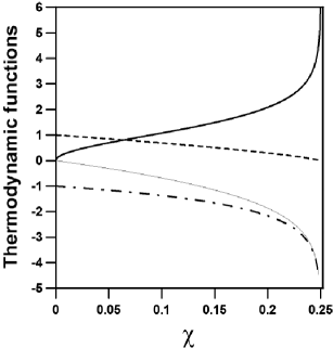
where this last thermodynamic definition for the entropy of course agrees with the previous Shannon expression in Eq.(38). To finished this section in Fig. 1 we present the dependence of these thermodynamic magnitudes with the interference parameter $\chi$.

IV Localized initial conditions

Figure 2: Isothermal curves as functions of the dimensionless angles $\gamma$ and $\varphi$. Due to the rotation symmetry in the angle $\varphi$, only four zones are distinguished: two ”cold” and two ”hot”. The ”hot” zones (orange on line) have six isotherms; from inside to outside their temperatures are: $T/T_{0}=6.5,~{}3.2,~{}2.2,~{}1.6,~{}1.3$ and $1.1$. The ”cold” zones (blue on line) have five isotherms; from outside to inside their temperatures are: $T/T_{0}=0.9,~{}0.8,~{}0.7,~{}0.68$ and $0.66$. The straight (green) lines corresponded to $T/T_{0}=1$, see Eq.(52).

Figure 3: The isothermal curves of Fig. 2 shown on the Bloch sphere. The QW initial chirality determines the entanglement temperature, see Eqs.(44,48,50).

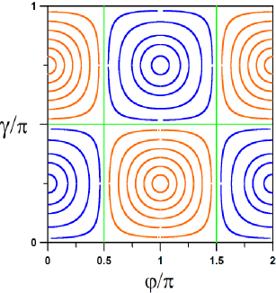
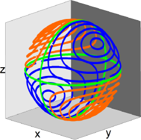
As seen in the previous section the thermodynamics of entanglement only depends on the interference term $Q_{0}$ which in turn only depends on the initial conditions, as shown in alejo2010 .

In order to investigate this dependence on the initial conditions of the system we consider first the localized case. The initial state of the walker is assumed to be sharply localized at the origin with arbitrary chirality, thus

$$|\Psi(0)\rangle=\left(\begin{array}[]{c}\cos({\gamma}/{2})\\ \exp i\varphi\text{ }\sin({\gamma}/{2})\end{array}\right)|0\rangle,$$ (48)

where $\gamma\in\left[0,\pi\right]$ and $\varphi\in\left[0,2\pi\right]$ define a point on the unit three-dimensional Bloch sphere. The expression of $Q_{0}$ was obtained in Ref. abal , fixing the bias of the coin toss $\theta=\pi/4$, following the method developed by Nayak and Vishwanath nayak

$$Q_{0}=\frac{1}{2}(1-\frac{1}{\sqrt{2}})\left[\cos\gamma\text{ }+\sin\gamma\text{ }(\cos\varphi+i\sqrt{2}\sin\varphi)\right].$$ (49)

Using this result in Eq.(35) the dependence of $\chi$ with the initial conditions is given by

$$\chi=\chi_{0}\left(1+\cos\varphi\sin 2\gamma\right),$$ (50)

where $\chi_{0}={3}/{4}-1/\sqrt{2}$.

It is useful to define a characteristic temperature (in units of $\epsilon$)

$$T_{0}=2/\left[\ln\left(\frac{1+2\sqrt{\chi_{0}}}{1-2\sqrt{\chi_{0}}}\right)\right],$$ (51)

in order to express any other temperature as a proportionality with $T_{0}=1/\beta_{0}$. Then from Eq.(44) we obtain an expression for $\beta$ as a function of the angles $\gamma$ and $\varphi$

$$\cos\varphi\sin 2\gamma=\left(\frac{\tanh\beta}{\tanh\beta_{0}}\right)^{2}-1.$$ (52)

Figures  2 and 3 show the level curves (isotherms) for the entanglement temperature as a function of the QW initial position. In Fig. 2 the initial position is defined through the angles $\gamma$ and $\varphi$ and in Fig. 3 it is defined through the position on the Bloch sphere (see Eq.(48)). Both figures show four regions, two of them corresponding to temperatures $T>T_{0}$ (orange color on line) and the other two to temperatures $T<T_{0}$ (blue color on line). The longest isotherms (green color on line) correspond to the temperature $T=T_{0}$ and their initial conditions are $\gamma=0,~{}\pi/2,~{}\pi$ and $\varphi=\pi/2,~{}3\pi/2$.

V Distributed initial conditions

Figure 4: Isothermal curves as functions of the dimensionless angles $\gamma$ (initial conditions) and $\theta$ (bias of the coin). Four curves (with different colors on line) are presented; each curve has two branches placed symmetrically on both sides of $\gamma=\pi/2$, where $T=\infty$. The values of $T$ are given by Eqs.(59). From left to right the values of $T$ are, in units of $\epsilon$: 0.5 (purple), 1. (blue), 2. (green) and 5. (orange). The diagram has two discontinuities in $\theta=\pi/2$ and in $\gamma=\pi/2$ (see Eqs.(59,60)).

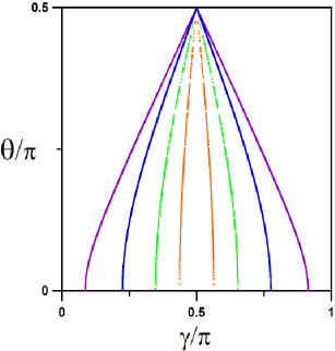
In previous works Eugenio ; alejo2010 we have studied the QW with extended initial conditions. Now the entanglement temperature is studied in such a case. The following extended Gaussian distributions is proposed:

$$a_{k}^{0}\equiv{\left[\frac{1}{\sigma_{0}\sqrt{2\pi}}\exp\left(-\frac{k^{2}}{2\sigma_{0}^{2}}\right)\right]}^{\frac{1}{2}}\cos({\gamma}/{2})\text{,}$$ (53)

$$b_{k}^{0}\equiv e^{i\varphi}{\left[\frac{1}{\sigma_{0}\sqrt{2\pi}}\exp\left(-\frac{k^{2}}{2\sigma_{0}^{2}}\right)\right]}^{\frac{1}{2}}\,\sin({\gamma}/{2})\text{,}$$ (54)

where $\sigma_{0}$ is the initial standard deviation, $\gamma\in\left[0,\pi\right]$ determines the initial proportion of the left and right chirality and $\varphi\in\left[0,2\pi\right]$ is a global phase. Using these initial conditions, Eqs.(53, 54), the asymptotic value of $Q(t)$, see Eqs.(15,24), was obtained alejo2010 as

$$Q_{0}=\frac{1}{2}\cos\gamma\,\tan\theta\,,$$ (55)

with the restrictions

$$\sigma_{0}\gg 1,$$ (56)

and

$$\cos\varphi=\frac{\tan\theta}{\tan\gamma}.$$ (57)

Replacing Eq.(55) in Eq.(35) we obtain

$$\chi=\left(\frac{\cos\gamma}{2\cos\theta}\right)^{2},$$ (58)

and then using Eq.(44) we have

$$\beta\epsilon=\frac{1}{2}\ln\left(\frac{\left|\cos\theta\right|+\left|\cos\gamma\right|}{\left|\cos\theta\right|-\left|\cos\gamma\right|}\right),$$ (59)

where taking into account Eqs.(37, 58) the initial condition satisfies the constraint

$${\left|\cos\gamma\right|}<{\left|\cos\theta\right|}.$$ (60)

The functions $Q_{0}$, $\chi$ and $\beta$ vanish for $\gamma=\pi/2$ ( see Eqs.(55, 58, 59)) and simultaneously the entanglement entropy Eq.(31) has its maximum value $S_{0}=1$. This maximum value is achieved when the entanglement temperature is $T=\infty$. Under these conditions the system behaves as a classical Markov process alejo2010 . On the other hand, the initial conditions $\gamma$ and $\varphi$ are not independent (see Eq.(57)) and for each value of $\gamma$ there is only one value of $T$, then for fixed $\theta$, it is not possible to have isotherms as functions of $\gamma$ and $\varphi$. Instead the entanglement temperature depends on $\theta$ and $\gamma$ from Eq.(59), i.e- the choice of the bias of the coin toss $\theta$ or of the initial proportion of the chirality $\gamma$ could lead to the same entanglement temperature. Fig. 4 shows the isotherms as functions of $\gamma$ and $\theta$.

VI Transient behavior

Figure 5: Envelope of the probability $\lambda_{+}-\Lambda_{+}$ as a function of the dimensionless time $t$ for two different initial conditions. Each initial condition is established by the couple $(\varphi,\gamma)$ in Eq. (48). Their values are $(\pi/8,\pi/4)$ for the full black line and $(\pi/4,\pi/3)$ for the dashed red line. In both cases, the temperature is $T=0.79~{}T_{0}$.

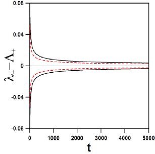
In the QW a stationary entanglement is established between the chirality and position degrees of freedom after a transient time. This fact allowed us to introduce the concept of entanglement temperature. The transient behavior of the system is studied using the original map Eq.(3) in a numerical code with initial conditions given by Eq.(48). These numerical calculations are summarized in Figs.  5 and  6. Fig. 5 presents the difference between the transient ($\lambda_{+}$) and the stationary ($\Lambda_{+}$) eigenvalues of the density matrix as a function of time (see Eqs.(30, 32)). The figure only presents the envelope of the curves because the real eigenvalues dynamics is very intricate; it presents quick oscillations with high density of paths where it is only possible distinguish its global contour. However, the average evolution of the system is determined by the envelope dynamics. Each envelope has two branches placed symmetrically on both sides of $\lambda_{+}-\Lambda_{+}=0$. Two pair of curves are presented in full and dashed lines with color black and red respectively. In both cases, the envelopes decay for $t\rightarrow\infty$ as a power law $1/t^{c}$ with $c=0.490$ for the dashed red line and $c=0.486$ for the full black line. The envelopes of $\lambda_{\pm}$ will be called $\widetilde{\lambda}_{\pm}$ respectively.

Figure 6: The power law exponent as a function of the dimensionless angle $\gamma$. The initial conditions $(\varphi,\gamma)$ correspond to the isotherms $T=1.1~{}T_{0}$.

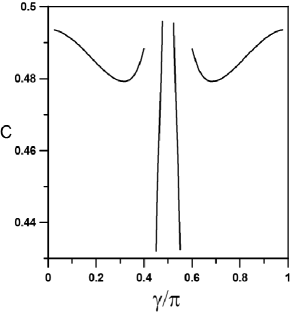
It was numerically verified for several initial conditions given by Eq.(48) that the transient behavior of $\widetilde{\lambda}_{\pm}-{\Lambda}_{\pm}$ can be adjusted by a power law function of time. Fig. 6 shows the power law exponent $c$ as a function of the initial condition $\gamma$ for the same temperature. Remember that, for $T$ and $\gamma$ given, $\varphi$ is determined by Eq.(52). Therefore, the exponent $c$ has a dependence with the initial conditions, however this dependence is not determined by the asymptotic temperature value.

Additionally, the transient behavior of $\widetilde{\lambda}_{\pm}-{\Lambda}_{\pm}$ was numerically studied, using initial conditions given by Eqs.(53, 54) with $\sigma\gg 1$. In these cases, the system showed a negligible transient dynamics, in concordance with the calculation developed in Ref. alejo2010 . Therefore, for these initial conditions, the reduced density matrix is essentially always in thermodynamic equilibrium.

With the aim to understand the transient behavior of the system we develop an analytic theory implementing a parallelism between the reduced density operator Eq.(42) and the density operator of an electron in a external magnetic field. With this picture on mind we propose the following master equation for the probabilities ${\lambda}_{+}$ and ${\lambda}_{-}$

$$\frac{d{\lambda}_{-}}{dt} ={\lambda}_{+}\,w_{+-}\,-{\lambda}_{-}\,w_{-+},\,$$

$$\frac{d{\lambda}_{+}}{dt} ={\lambda}_{-}\,w_{-+}\,-{\lambda}_{+}\,w_{+-},$$ (61)

where $w_{+-}$ and $w_{-+}$ are transition probabilities per unit of time, that can be understood as population rates. $w_{+-}$ corresponds to the transition ${\lambda}_{+}\rightarrowtail{\lambda}_{-}$ and $w_{-+}$ corresponds to the transition ${\lambda}_{-}\rightarrowtail{\lambda}_{+}$. These rates are time-dependent functions, and their behaviors are known in the limit $t\rightarrow\infty$ when ${d{\lambda}_{\pm}}/{dt}\longrightarrow 0$. In this limit, the stationary solution of Eq.(61) must be the couple $\Lambda_{-}$ and $\Lambda_{+}$, given by Eq.(32). Then the asymptotic values of the population rates satisfy

$$\frac{w_{b}}{w_{a}}=\frac{\Lambda_{-}}{\Lambda_{+}},$$ (62)

where $w_{a}$ and $w_{b}$ are defined by

$$w_{a} \equiv\begin{array}[]{c}\lim\text{ }w_{-+}\\ t\rightarrow\infty{}{}{}\end{array},\,$$ (65)

$$w_{b} \equiv\begin{array}[]{c}\lim\text{ }w_{+-}\\ t\rightarrow\infty{}{}{}\end{array}.\,$$ (68)

Eq.(62) expresses a condition of detailed balance which says that the rate of occurrence for any transition equals the rate for the inverse transition. Using our knowledge about the transient and asymptotic behaviors, the following population rates are proposed

$$w_{+-}=w_{b}+\xi(t),\,$$ (69)

$$w_{-+}=w_{a}-\xi(t),\,$$ (70)

where

$$\xi(t)=\frac{K}{t^{c}}[\omega\sin(\omega t+\delta)+(\frac{c}{t}-w_{a}-w_{b})\cos(\omega t+\delta)],$$ (71)

with $c>0$, $K$, $\omega$ and $\delta$ constants. The general solution of Eq.(61) with these population rates is

$${\lambda}_{+}=\Lambda_{+}+\frac{K}{t^{c}}\cos(\omega t+\delta)+d\,e^{-(w_{a}+w_{b})t},\,$$ (72)

$${\lambda}_{-}=\Lambda_{-}-\frac{K}{t^{c}}\cos(\omega t+\delta)-d\,e^{-(w_{a}+w_{b})t},\,$$ (73)

where $d$ is an additional constant. Note that $e^{-(w_{a}+w_{b})t}\rightarrow 0$ faster than ${1/t^{c}}$ for $t\rightarrow\infty$, then Eqs.(72,73) verify the asymptotic behavior obtained numerically. All the constants $K$, $c$, $\omega$, $\delta$ and $d$ depend on the initial conditions, however their values should be compatible with the positive character of the functions $\lambda_{+}$, $\lambda_{-}$, $w_{+-}$ and $w_{-+}$. In particular, to describe correctly the numerical results, $K$ takes a finite value for localized initial conditions and $K$ takes negligible value for distributed initial conditions. In summary, the Brownian motion equation for our reduced density matrix Eq.(39), takes the form of a master equation Eq.(61).

Finally it is important to point out that the asymptotic behavior found here is similar to the behavior of the simple cellular automaton known as sandpile btw . Such behaviors are characteristic of extended dynamical systems with spatial degrees of freedom. They naturally evolve to self-organized states with correlations that decay with a power law.

VII Conclusion

The unitary evolution of the QW in a composite Hilbert space is studied. In particular the entanglement between chirality and position degrees of freedom is investigated. After a transient time the system establishes a stationary entanglement between the coin and the position that allows to develop a thermodynamic theory. The asymptotic reduced density operator is used to introduce the entanglement thermodynamic functions in the canonical equilibrium. These thermodynamic functions characterize the asymptotic entanglement. It is shown that the QW initial condition determines the system’s temperature, as well as other thermodynamic function. A map for the isotherms is analytically built for arbitrary localized initial conditions. Additionally, it is shown that choosing appropriately the bias of the coin-toss, it is possible to obtain a predetermined entanglement temperature.

The transient dynamics of the reduced density operator outside the thermodynamic equilibrium is also studied. We show numerically that this transient behavior can be adjusted with a power law, whose exponent depends on the initial conditions. We built a master equation to describe this behavior where the population rates have a time dependence. The accuracy of the master equation solution is numerically verified and it is shown that the reduced density has a cellular automaton behavior.

The behavior of the reduced density operator looks diffusive but it has a dependence with the initial conditions, the global evolution of the system is unitary. Then, if an observer only had information related with the chirality degrees of freedom, it would be very difficult for him to recognize the unitary character of the quantum evolution. In general, from this simple model we can conclude that if the quantum system dynamics is developed in a composite Hilbert space, then the behavior of operators that only belong to one sub-space could camouflage the unitary character of the global evolution.

I acknowledge stimulating discussions with Víctor Micenmacher, Guzmán Hernández, Raúl Donangelo and Armando Pérez and the support from PEDECIBA and ANII.

References

- (1) Y. Aharonov, L. Davidovich, and N. Zagury, Phys. Rev. A 48, 1687 (1993); D. A. Meyer, J. Stat. Phys. 85, 551 (1996); J. Watrous, Proc. STOC’01 (ACM Press, New York, 2001), p.60; A. Ambainis, Int. J. Quant. Inf. 1, 507 (2003); J. Kempe, Contemp. Phys. 44, 307 (2003); V. Kendon, Math. Struct. Comp. Sci. 17, 1169 (2006); V. Kendon, Phil. Trans. R. Soc. A 364, 3407 (2006); N. Konno, Quantum Walks, in Quantum Potential Theory, Lect. Notes Math., Vol. 1954, edited by U. Franz and M. Schürmann (Springer, 2008); A. Wojcik, T. Luczak,P. Kurzynski, A. Grudka, M. Bednarska, Phys. Rev. Lett. 93, 180601 (2004); M.C. Bañuls, C. Navarrete, A. Pérez, E. Roldán, and J.C. Soriano, Phys. Rev. A 73, 062304 (2006), A. Romanelli, A. Auyuanet, R. Siri, G. Abal, and R. Donangelo, Physica A 352, 409 (2005).
- (2) A.M. Childs, Phys. Rev. Lett. 102, 180501 (2009).
- (3) A. Romanelli, Phys. Rev. A, 80, 042332 (2009).
- (4) N. Linden, and J. Sharam, Phys. Rev. A, 80, 052327 (2009).
- (5) N. Shenvi, J. Kempe, K. BirgittaWhaley, Phys. Rev. A 67, 052307 (2003).
- (6) A. Childs, E. Deotto, E. Farhi, S. Gutmann, and D. A. Spielman, in Proc. 35th ACM Symposium on Theory of Computing (STOC 2003), pp. 59–68, 2003, arXiv preprint quant-ph/0209131.
- (7) A. Romanelli, Phys. Rev. A 81, 062349 (2010).
- (8) A. Romanelli, Physica A, 390, 1209 (2011).
- (9) A. Pérez, and A. Romanelli, in preparation (2011).
- (10) A. Romanelli, Phys. Rev. A 80, 042332 (2009).
- (11) A. Romanelli, A.C. Sicardi Schifino, R. Siri, G. Abal, A. Auyuanet, and R. Donangelo, Physica A, 338, 395 (2004).
- (12) A. Romanelli, A.C. Sicardi Schifino, G. Abal, R. Siri, and R. Donangelo, Phys. Lett. A 313, 325 (2003).
- (13) A. Romanelli, R. Siri, G. Abal, A. Auyuanet, and R. Donangelo, Physica A, 347, 395 (2005).
- (14) D. Aharonov, A. Ambainis, J. Kempe, and U. Vazirani, Proc. of the 33rd Annual ACM STOC, ACM, NY, 50 (2001). arXiv preprint quant-ph/0001.2090v2 (2002).
- (15) I. Carneiro, M. Loo, X. Xu, M. Girerd, V. M. Kendon, and P. L. Knight, New J. Phys. 7, 56 (2005).
- (16) G. Abal, R. Siri, A. Romanelli, and R. Donangelo, Phys. Rev. A 73, 042302, 069905(E) (2006).
- (17) M. Annabestani, M. R. Abolhasani and, G. Abal, J. Phys. A: Math. Theor. 43, 075301 (2010).
- (18) Y. Omar, N. Paunkovic, L. Sheridan, and S. Bose, Phys. Rev. A, 74, 042304 (2006)
- (19) P. K. Pathak, and G. S. Agarwal, Phys. Rev. A, 75, 032351 (2007)
- (20) C. Liu, and N. Petulante, Phys. Rev. A 79, 032312 (2009).
- (21) S. E. Venegas-Andraca, J.L. Ball, K. Burnett, and S. Bose, New J. Phys., 7, 221 (2005).
- (22) J. Endrejat, H. Büttner, J. Phys. A: Math. Gen. 38, 9289 (2005).
- (23) A.J. Bracken, D. Ellinas, and I. Tsohantjis, J. Phys. A: Math. Gen. 37, L91 (2004).
- (24) D. Ellinas, and A.J. Bracken, Phys. Rev. A 78, 052106 (2008).
- (25) O. Maloyer, and V. Kendon, New J. Phys., 9, 87 (2007).
- (26) S. E. Venegas-Andraca , and S. Bose, arXiv preprint quant-ph/0901.3946v1 (2009).
- (27) S. Goyal, and C. M. Chandrashekar, arXiv preprint quant-ph/0901.0671 (2009).
- (28) R. Kubo, M. Toda, and N. Hashitsume Statistical Physics II, Nonequilibrium Statistical Mechanics, Springer-Verlag, Berlin Heidelberg New York Tokyo; ISBN 3 540 11461 0, (1985).
- (29) 10 A. Nayak and A. Vishwanath, e-print quant-ph/0010117
- (30) G.J.de Valcárcel, E. Roldán and A. Romanelli, New Journal of Physics 12, 123022 (2010).
- (31) R. K. Pathria Statistical Mechanics , secon edition,ISBN 0 7506 2469 8, (1997).
- (32) H. J. Jensen, Self-Organized Criticality, first edition, ISBN 0 521 48371 9 (1998).