Entropy and equilibrium state of free market models

Abstract

Many recent models of trade dynamics use the simple idea of wealth exchanges among economic agents in order to obtain a stable or equilibrium distribution of wealth among the agents. In particular, a plain analogy compares the wealth in a society with the energy in a physical system, and the trade between agents to the energy exchange between molecules during collisions. In physical systems, the energy exchange among molecules leads to a state of equipartition of the energy and to an equilibrium situation where the entropy is a maximum. On the other hand, in the majority of exchange models, the system converges to a very unequal condensed state, where one or a few agents concentrate all the wealth of the society while the wide majority of agents shares zero or almost zero fraction of the wealth. So, in those economic systems a minimum entropy state is attained. We propose here an analytical model where we investigate the effects of a particular class of economic exchanges that minimize the entropy. By solving the model we discuss the conditions that can drive the system to a state of minimum entropy, as well as the mechanisms to recover a kind of equipartition of wealth.

1 Introduction

The second law of thermodynamics states that isolated systems always tend to an equilibrium state of maximum entropy, where equilibrium means that the macroscopic properties of the system are the same in any part of it. The second law of thermodynamics can also be deduced from an analysis of the efficiency of a thermal engine, and according to Clausius: “No process is possible whose sole result is the transfer of heat from a body of lower temperature to a body of higher temperature” [1] In modern statistical physics the second law may be inferred from Boltzmann H-theorem [1] and it is generally accepted as a natural consequence of the energy exchange among molecules in the kinetic theory of gases: when molecules collide in a gas there is a transfer of kinetic energy from the more energetic to the less energetic molecules and, as a consequence, after a transient, all molecules share, in average, the same energy. This result is the theorem of equipartition of energy that characterizes the Maxwell-Boltzmann equilibrium distribution of velocities, and it is associated with the maximum entropy state. However, in particular situations, it may happen that the entropy decreases as a function of time; examples are self-organized systems and biological organisms. One common characteristic of those systems is that they are not in equilibrium even if they seem stable or stationary in time [2].

The idea that economic systems also possess some kind of equilibrium state is an underlying concept in classical economic theory, going from Pareto optimality to Nash equilibrium [3]. The Edgeworth box model is an example of how a simple exchange conservative model can lead two consumers to optimize their respective utility [3]. But in other cases there are symptomatic evidences that economic systems can be out of equilibrium and/or exhibit metastable equilibrium states. This is the case when studying the wealth and income distribution. Fluctuations around an equilibrium state behave in a Gaussian or normal way: The probability of rare events is very small, as the Gaussian distribution exhibits exponential tails. On the other hand, empirical studies focusing the income distribution of workers, companies and countries were first presented more than a century ago by Vilfredo Pareto and he discovered that the income distribution does not behave in a Gaussian way but exhibits “heavy tails”, i.e. the cumulative probability $P(w)$ of workers whose income is at least $w$ follows a power law [4] given by $P(w)\propto w^{-\beta}$. Nowadays, this power law distribution is known as Pareto distribution, and the corresponding exponent $\beta$ is named Pareto exponent. However, recent data indicates that, even though Pareto distribution provides a good fit in the high income range, it does not agree with the observed data over the middle and low income range. For instance, data from Japan [5, 6], Italy [7], India [8], the United States of America and the United Kingdom [9, 10, 11] are fitted by a log-normal or Boltzmann distribution with the maximum located at the middle-income region plus a power law for the high-income strata. The existence of these two regimes may be justified in a qualitative way by stating that in the low and middle income classes the process of wealth accumulation is additive (and mainly due to wages), causing a Gaussian-like distribution, while in the high income range, wealth grows in a multiplicative way, generating the observed power law tail [6].

In recent years physicists and economists working in complexity science proposed different mathematical models of wealth exchange among economic agents in order to try to explain these empirical data (For a review see refs. [12, 13, 14]). Quoting ref. [12]: Inspired by Boltzmann’s kinetic theory of collisions in gases, econophysicists introduced an alternative two-body approach, where agents perform pairwise economic transactions and transfer money from one agent to another. Actually, this approach was pioneered by the sociologist John Angle [15, 16]. Most of these models consider an ensemble of interacting economic agents, each one possessing a given amount of endowments, money[9] or assets[14, 17] that represents its economics resources and that we will describe as “wealth”. Most of these models focus on one particular aspect of economic processes: The competition among different agents (countries, enterprises, etc.) acting in an environment where all exchanges of wealth between agents take place in a conservative manner, i.e., a conservative exchange market model (CEMM)˜[18]. This restriction has several motivations: On the one hand, it can be argued that resources are material objects, and consequently they cannot be created or destroyed by means of exchanging them. On the other hand, the use of the CEMM implies that the exchange model is a zero-sum game, something that may seem at odds with usual economic orthodoxy. However, the results also hold for systems in which the total amount of wealth increases uniformly and smoothly in time. The interaction among agents consists in a exchange of a fixed [9] or random [14, 17] amount of their wealth. The process of exchange is similar to the collision of molecules in a gas and the amount of exchanged wealth when two agents interact corresponds to some economic “energy” that may be transferred for one agent to another. If this exchanged amount corresponds to a fixed or random fraction of one of the interacting agents wealth, the resulting wealth distribution is – unsurprisingly – a Gibbs exponential distribution [9].

Aiming at obtaining distributions with power law tails, in order to describe the higher income region of the wealth distribution histogram, several methods have been proposed mostly introducing a multiplicative risk aversion that acts as a multiplicative noise. Numerical results[14, 17, 20, 21, 22, 23, 24], as well as some analytical calculations [25, 26], indicate that a frequent outcome in these models is condensation, i.e. concentration of all available wealth in just one or a few agents. This final state corresponds to a kind of equipartition of poverty: All agents (except for a set of zero measure) possess zero wealth while one, or a few ones, concentrate all available resources. In any case the final configuration is a stationary state of “equilibrium”, since agents with zero wealth cannot participate in further exchanges. Several methods have been proposed to avoid this situation, for instance, exchange rules where the poorer agents are favored [8, 14, 24, 26, 27] or taxes and regulations [28, 29]. Here, instead, we are mainly interested in the condensed state and in the dynamics driving the system to this condensed state, as well as in the entropy behavior when the system approaches condensation.

As previously stated, exchange rules are determinant of the long-time behavior of the system. While we can obtain an exponential Boltzmann-Gibbs distribution - and consequently a maximum entropy state - if the exchanged fraction is fixed or determined at random, condensation is the outcome when exchange rules are so that, when two agents interact, the exchanged amount $\Delta w$ is proportional to the wealth of one of the participants or to both [25] but in no case one participant can win more that the value he put in stake. So, the exchange process is a kind of lottery where no agent can win more than his own possessions. One particular and widely used exchange rule is to consider that the fraction of transferred wealth from agent $x^{\prime}$ to agent $x^{\prime\prime}$, or vice versa, is: $\Delta w=\mbox{min}\{(1-\lambda)w^{\prime};(1-\lambda)w^{\prime\prime}\}$, where $w^{\prime}$ and $w^{\prime\prime}$ are the respective wealth of the two interacting agents, and $\lambda$ is a risk-aversion factor, so the capital fraction that the agents risk during the exchange is $1-\lambda$ [14, 24, 26]. It is worth noting that even approaching a condensed state, in the intermediate stages the wealth distribution goes through a series of power law distributions where the Pareto exponent increases as a function of time [26]. The problem with the previous definition of $\Delta w$ is that it involves a logical comparison that is difficult to be treated analytically. Here we consider another form of $\Delta w$. We define an analytical expression of $\Delta w$ that guarantees that no agent participating in the exchange risk more than the quantity he can win. To do that we define $\Delta w=\frac{w^{\prime}w^{\prime\prime}}{w^{\prime}+w^{\prime\prime}}$, that presents similar properties and is equal to the wealth of the poorer partner when the wealth of the richer agents is much bigger than the other. Notice also that we eliminated the risk-aversion factor, just by considering $\lambda=0$, because we have verified that one does not need the multiplicative noise to obtain the condensed state. Using this exchange rule and the methods of non-equilibrium statistical mechanics we show in this paper that the entropy decreases in the intermediate stages leading to a condensed state of minimum entropy (and maximum inequality, Gini coefficient equal to 1).

The text is organized as follows: in the next section we write the exchange model in the form of a master equation that is solved by numerical iteration in section 3. Next in section 4 we calculate the entropy of the system as well as the Theil coefficient and we discuss why in this case the Boltzmann H-theorem is not verified. Finally the results are discussed and the conclusions presented in section 5.

2 The evolution equation

We consider a collection of $R$ individuals, each one characterized by a given value of a continuous variable $w$. This variable can represent the wealth, cash, properties, or some other measure of the agent’s fortune, but it can also represent a physical scalar quantity, as energy. Like in the kinetic theory of gases, agents may interact and exchange any fraction of $w$. In the standard kinetic theory the exchange of random fractions of energy leads to an equilibrium state described by Maxwell-Boltzmann distribution[1]. In the same way, considering $w$ as representing the money owned by an agent, and random exchanges between agents, a maxwellian money distribution is also found[9, 10, 18, 19]. However, as previously stated, different exchange mechanisms can be considered. Several of them are in some way proportional to the wealth owned by the participating agents and leads to a condensed state[14, 19, 21, 22, 23, 24, 25]. Here we study a very simple non-linear exchange rule. Let us consider two agents, with wealth $w^{\prime}$ and $w^{\prime\prime}$, respectively. We assume that when they interact they exchange $\Delta w=(w^{\prime}w^{\prime\prime})/(w^{\prime}+w^{\prime\prime})$. It implies that when the two agents have very similar wealth, the exchanged amount is approximately half of each agent wealth, while if the possessions are very different, the transferred amount is equal to the poorer agent’s wealth. This expression yields a fair exchange rule in the sense that no agent risks more that the amount he can win. Indeed the rule is very similar to the one used in refs. [14, 24], i.e. $w=\mbox{min}\{w,w^{\prime}\}$ but here we avoid the logical operator using an analytical expression.

We also aim at investigating the effect of favoring the poorer agent in an interaction. Condensation of wealth is an undesirable effect in models describing wealth distribution and many authors proposed different ingredients to avoid this effect. One of the most popular recipes is to define a wealth-dependent probability of winning a transaction. For example in refs. [8, 14, 24, 26, 27] it is assumed that the winning probability is higher for the poorer participating agent. Even if this recipe seems counterintuitive, favoring the poorer agent in every transaction somehow emulates a regulatory policy imposed by a government. To assess the effects of this kind of policy, we assume that in an interaction between two agents with wealth $w^{\prime}$ and $w^{\prime\prime}$, the probability $p_{\gamma}(w^{\prime}|w^{\prime\prime})$ that the agent with wealth $w^{\prime}$ wins the exchanged amount, $\Delta w=(w^{\prime}w^{\prime\prime})/(w^{\prime}+w^{\prime\prime})$, is given by

$$p_{\gamma}(w^{\prime}|w^{\prime\prime})=\frac{1}{2}\left[1-\gamma\tanh\left(w^{\prime}-w^{\prime\prime}\right)\right],$$ (1)

where $\gamma$ may assume any value in the interval $[0,1]$. This winning probability has the following properties

• $p_{\gamma}(w^{\prime}|w^{\prime\prime})=\frac{1}{2}$, if $w^{\prime}=w^{\prime\prime}$ for all $\gamma$.

• $p_{\gamma}(w^{\prime}|w^{\prime\prime})=\frac{1}{2}$, if $\gamma=0$ for all $w^{\prime}$ and $w^{\prime\prime}$.

• $p_{\gamma}(w^{\prime}|w^{\prime\prime})=\frac{1}{2}(1\mp\gamma)$, if $w^{\prime}-w^{\prime\prime}\rightarrow\pm\infty$, so $0\leq\gamma\leq 1$.

• $p_{\gamma}(w^{\prime}|w^{\prime\prime})+p_{\gamma}(w^{\prime\prime}|w^{\prime})=1$, for all $0\leq\gamma\leq 1$, $w^{\prime}$, and $w^{\prime\prime}$.

Hence, by varying $\gamma$ we can investigate the effects of a varying the winning probability on the wealth distribution.

We define $N(w,t)dw$ as the probability of finding an agent with wealth in the interval $[w,w+dw]$ at time $t$ or, alternatively, as the relative number of agents with wealth in that interval. From now on, we consider the limit where there is an infinite number of agents, such that $N(w,t)$ is a continuous function of $w$. The wealth evolution of such agents depend on their transactions. Assuming that i) the probability per unit time that two agents of wealth $w$ and $w^{\prime}$ perform a transaction is given by $k\;N(w,t)\,N(w^{\prime},t)\,dw\,dw^{\prime}$, with $k$ being the transaction frequency; ii) the exchanged wealth in that transaction is $\Delta w=(w^{\prime}w^{\prime\prime})/(w^{\prime}+w^{\prime\prime})$; and iii) the probability of gaining or loosing that amount is given by a regulatory function $p_{\gamma}(w^{\prime}|w^{\prime\prime})$ given by Eq.(1); we may write the evolution equation for $N(w,t)$ as

$$N(w,t+\Delta t)-N(w,t)=-2\;k\;N(w,t)$$

$$+k\;\int_{0}^{\infty}{dw^{\prime}}\int_{0}^{\infty}{dw^{\prime\prime}}N(w^{\prime},t)N(w^{\prime\prime},t)\left\{p_{\gamma}(w^{\prime}|w^{\prime\prime})\;\delta\left(w-\left[w^{\prime}+\frac{w^{\prime}\;w^{\prime\prime}}{w^{\prime}+w^{\prime\prime}}\right]\right)\right.$$

$$+\left.p_{\gamma}(w^{\prime\prime}|w^{\prime})\;\delta\left(w-\left[w^{\prime}-\frac{w^{\prime}\;w^{\prime\prime}}{w^{\prime}+w^{\prime\prime}}\right]\right)+p_{\gamma}(w^{\prime\prime}|w^{\prime})\;\delta\left(w-\left[w^{\prime\prime}+\frac{w^{\prime}\;w^{\prime\prime}}{w^{\prime}+w^{\prime\prime}}\right]\right)\right.$$

$$+\left.p_{\gamma}(w^{\prime}|w^{\prime\prime})\;\delta\left(w-\left[w^{\prime\prime}-\frac{w^{\prime}\;w^{\prime\prime}}{w^{\prime}+w^{\prime\prime}}\right]\right)\right\}.$$ (2)

This is a non-linear probability conservation equation. The first term in the right hand side of Eq.(2) gives the amount of agents that have changed from $w$ to some other value. This term is proportional to the total number $K(w)$ of transactions involving agents with wealth in the range $(w,w+dw)$, during the time interval $dt$, which is given by

$$K(w) = k\int_{0}^{\infty}{dw^{\prime}}\int_{0}^{\infty}{dw^{\prime\prime}}N(w^{\prime},t)N(w^{\prime\prime},t)\left[\delta(w^{\prime}-w)+\delta(w^{\prime\prime}-w)\right]$$

$$= 2\;k\;N(w,t),$$

and where we have explicitly taken into account the normalization of $N(w,t)$, that is, $\int_{0}^{\infty}{dw}N(w,t)=1$. The other four terms in Eq.(2) describe the increment in $N(w,t)$ due to agents that changed their wealth to $w$ (by winning money, first and third terms, or by losing money, second and fourth terms) during $dt$. The conservation of number of agents is easily verified by integrating Eq.(2) in $w$. The total wealth is also conserved. As the number of agents is conserved, wealth conservation is demonstrated by showing that the time derivative of the average wealth is zero:

$$\frac{\mbox{d}}{\mbox{d}t}\langle w\rangle=\int_{0}^{\infty}dw\;w\frac{\partial N(w,t)}{\partial t}=0,$$ (4)

Using Eq.(2) to estimate the time derivative of $N(w,t)$ and performing the integrals containing $\delta$-functions we obtain

$$\int_{0}^{\infty}dw\;w\left[N(w,t+\Delta t)-N(w,t)\right]=$$

$$-2k\int_{0}^{\infty}dw\;wN(w,t)+\int_{0}^{\infty}{dw^{\prime}}\int_{0}^{\infty}{dw^{\prime\prime}}N(w^{\prime},t)N(w^{\prime\prime},t)k\times$$

$$\left\{p_{\gamma}(w^{\prime}|w^{\prime\prime})\left[w^{\prime}+\frac{w^{\prime}\;w^{\prime\prime}}{w^{\prime}+w^{\prime\prime}}\right]+p_{\gamma}(w^{\prime\prime}|w^{\prime})\left[w^{\prime}-\frac{w^{\prime}\;w^{\prime\prime}}{w^{\prime}+w^{\prime\prime}}\right]\right.$$

$$\left.+p_{\gamma}(w^{\prime\prime}|w^{\prime})\left[w^{\prime\prime}+\frac{w^{\prime}\;w^{\prime\prime}}{w^{\prime}+w^{\prime\prime}}\right]+p_{\gamma}(w^{\prime}|w^{\prime\prime})\left[w^{\prime\prime}-\frac{w^{\prime}\;w^{\prime\prime}}{w^{\prime}+w^{\prime\prime}}\right]\right\}=0,$$ (5)

implying a constant average wealth. We use wealth and number of agents conservation to define the wealth unit as the average wealth given by $\langle w\rangle=\int_{0}^{\infty}{dw}w\;N(w,t)/\int_{0}^{\infty}{dw}N(w,t)$. In what follows wealth is given in units of average wealth $\langle w\rangle$.

3 Numerical iteration

The evolution equation, Eq.2, has been numerically iterated by dividing the $w$ axis in bins of width $<w>/100$, while the exchange rate $k$ is taken as $k=0.01/\tau$ with $\tau$ being the simulation time step. We have considered two different initial conditions:

• a normal distribution with average $\langle w\rangle$ and variance $\langle w\rangle/6$.

• an uniform distribution in the interval $[0,2\langle w\rangle]$.

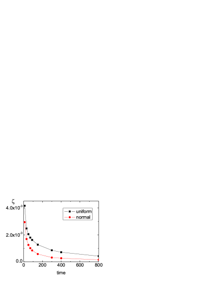
We first analyze the symmetric case, where $\gamma=0$, such that in each transaction the winning probability is 1/2 for both agents. Fig. 1 shows the time evolution in both cases, Fig. 1(a) for a normal initial distribution and Fig. 1(b) for a uniform initial distribution. It is interesting to note that after some initial oscillations, more pronounced for the case of the normal distribution (because at the beginning of the simulation the exchanged amounts are always very near $<w>/2$) the system arrives to the same distribution. This final distribution evolves to the condensed state. It is characterized by a very small fraction of agents with wealth above $<w>$, and an ever increasing number of agents with wealth very near zero. However, it is worth to note that the transient states present a clear exponential tail (and not power law), as one can see in the log-linear plots presented in Fig. (2, where the distributions are represented by a linearly decreasing function with an slope, $-\zeta$, that corresponds to the exponent of the distribution. This exponent decreases with time as shown in Fig. (2). One expects that for $t\rightarrow\infty$ the exponent goes to zero, indicating that all the agents have zero wealth. Nevertheless, as the total wealth is conserved a finite set of agents (one or a few, but in any case a zero-measure set) possess all the available resources On the other hand, the interval on the $w$ axis where $N(w,t)$ is described by an exponential increases with time, and ranges from $w$ of the order of $\langle w\rangle$ to a higher value of $w$ that increases in time. After that, $N(w,t)dw$ decreases very fast to values much smaller than $10^{-9}$ implying that it is very unlikely that a system described by that $N(w,t)$ would present agents in the high wealth interval. We call this distribution, where the number of agents goes to infinity for $w$ going to zero, and goes to zero for any finite wealth, an $L-$shaped distribution.

Figure 1: Plot of the wealth distribution at different times for (a) an initial normal distribution, (b) an initial uniform distribution.

Figure 2: Log-linear plot of the wealth distribution at different times for (a) an initial normal distribution, (b) an initial uniform distribution.

Figure 3: The exponent of the wealth distribution as a function of time for different initial conditions.

Condensation of wealth is an effect undesirable in models describing wealth distribution as well as in real societies. So, many authors proposed different mechanisms in order to avoid or compensate this effect. One of the most “popular” recipes is to define a wealth-dependent probability of being the winner in the transaction. For example in refs. [27, 24, 14, 8, 26] it is assumed that the probability of being the winner in a transaction is higher for the agent with the lower wealth in each interaction. Even if this recipe seems counterintuitive, increasing the probability of favoring the poorer agent is a way to simulate the action of the state or of some another type of regulatory tool aiming to redistribute the resources. In order to verify the effect of this kind of measure, here we will consider an asymmetric winning probability, by taking $0\leq\gamma\leq 1$ in Eq.(1). The iteration results for a uniform initial distribution are shown in Fig. 4, where we extended the iteration time from 800 to 3200 timesteps. The results for other initial conditions are similar, as it was for the $\gamma=0$ case. However, even considering values of $\gamma\neq 0$, as time evolves the distribution $N(w)$ tends to an L-shaped distribution where all agents concentrate at $w=0$, with an infinitesimal number of agents presenting $w>0$: all distributions exhibit peaks for $w=0$ as time increases. The exception happens for $\gamma=1$, when the peak in the distribution located at $w>0$, is stable and increases as time goes by. In this case the wealth distribution approaches a shape that is well fitted by a Gaussian or lognormal function. Nevertheless, it is clear from Fig. 4 that for bigger enough values of $\gamma$ the time for arriving to condensation is also bigger, so, for finite periods of time, increasing $\gamma$ diminish inequality.

Figure 4: Plot of the wealth distribution for $0<\gamma\leq 1$ at different times for an initial normal distribution.

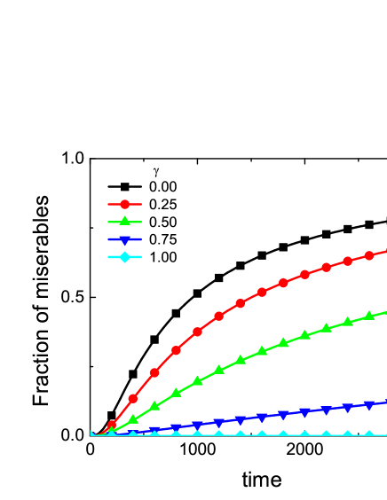
The fact that for $\gamma<1$ the system converges to condensation when $t\rightarrow\infty$ can be explained because when an agent reaches the miserable state, with $w\cong 0$, it no longer participates in the transactions, since in transactions involving $w=0$-agents the exchanged amounts are always zero. It means that the $w=0$ state acts as a trap of zero escaping probability: and it is just a question of time for the system to reach a state where all agents concentrate at the total misery state. The only case when this situation does not happen is when $\gamma=1$ because, in this case, the poorer agent always wins such that the system is driven towards a kind of equipartition of wealth. Fig. 5 illustrates this point by presenting the evolution of $N(w=0)$ with time, for different values of $\gamma$. The fraction of miserable agents remains finite, as in the initial state, only for $\gamma=1$.

Figure 5: Plot of $N(w=0)$ with time for normal initial condition and different values of $\gamma$

.

3.1 Entropy evolution: the second law

To quantitatively characterize the degree of inequality of the distribution we consider different estimators. Inequality is generally estimated by either using Gini coefficient [31], whose calculation is presented at the end of this section, or the Shannon entropy, known by economists as the Theil coefficient [32]. Here, in order to compare with a more typical thermodynamical variable, we also calculate the usual entropy of the system. We begin by calculating the conventional entropy, in the way it is defined in Statistical Physics textbooks [1]:

$$S=-\int_{0}^{\infty}N(w,t)\log{N(w,t)}.$$ (6)

The time evolution of the entropy is given by

$$\frac{\mbox{d}S}{\mbox{d}t} = -\frac{\mbox{d}}{\mbox{d}t}\int_{0}^{\infty}N(w,t)\log{N(w,t)}$$ (7)

$$= \int_{0}^{\infty}\frac{\partial N(w,t)}{\partial t}\log{N(w,t)}$$

and using equation 2, we obtain

$$\frac{dS}{dt} = -k\int_{0}^{\infty}{dw^{\prime}}\int_{0}^{\infty}{dw^{\prime\prime}}N(w^{\prime},t)N(w^{\prime\prime},t)$$

$$\times \log{\left[\frac{N\left(w^{\prime}+\frac{w^{\prime}w^{\prime\prime}}{w^{\prime}+w^{\prime\prime}},t\right)^{1-\gamma\tanh(w^{\prime}-w^{\prime\prime})}N\left(w^{\prime}-\frac{w^{\prime}w^{\prime\prime}}{w^{\prime}+w^{\prime\prime}},t\right)^{1+\gamma\tanh(w^{\prime}-w^{\prime\prime})}}{N(w^{\prime}t)N(w^{\prime\prime},t)}\right]}$$

Even if, for $\gamma=0$, a Boltzmann-like distribution with an effective temperature proportional to $<w>$, that is, $N(w)=\frac{\mbox{e}^{-\frac{w}{\langle w\rangle}}}{\langle w\rangle}$, yields $\frac{\mbox{d}S}{\mbox{d}t}=0$, a visual inspection of Fig.  2 suggests that this is not the stationary solution for long times even for $\gamma\neq 0$: the wealth distribution clearly exhibits an exponential behavior for intermediate and low values of $w$. Alternatively, there exists another type of function that presents norm $1$, average $\langle w\rangle=1$, and leads to $\frac{\mbox{d}S}{\mbox{d}t}=0$. This function is also compatible with the asymptotic stationary solution (as indicated by numerical simulations for $\gamma<1$), and is a stationary solution of Eq..(2). One possible function with these properties type is:

$$N_{st}(w,t)=\lim_{w_{max}\rightarrow\infty}\left\{\begin{array}[]{ll}1-\frac{2\langle w\rangle}{w_{max}}&\mbox{ if }w=0\\ \frac{2\langle w\rangle}{w_{max}^{2}}&\mbox{ if }0<w\leq w_{max}\\ 0&\mbox{ if }w>w_{max}\\ \end{array}\right.$$ (11)

This solution describes condensation that, even if from an economic point of view is the worst possible scenario, corresponds to the numerical results obtained in this work as well as in the references quoted above. The solution is also the attractor of the dynamic of the system:

• Due to the dynamics of the system $w_{max}$ is always increasing. So it tends to infinity for time going to infinity.

• The fraction of the agents populations with $w=0$ grows as $1-\frac{2\langle w\rangle}{w_{max}}$ and hence tends to 1 as $w_{max}\rightarrow\infty$.

• The total wealth concentrates in the infinitesimal population fraction, given by $\frac{2\langle w\rangle}{w_{max}}$ having $w>0$, which goes to zero as time goes to infinity.

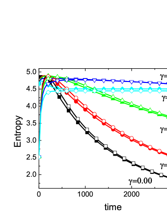
We call this solution “condensate solution”. The entropy evolution for the iterated distributions is presented in Fig.  6. For $\gamma<1$ the entropy initially increases, corresponding to the spreading of the distribution function. However, when the number of agents with zero wealth increases to very high values, the entropy decreases, indicating an ordered state: condensation of the agents in the $w=0$ state. This is compatible with the proposed attractor, Eq.. 11. It is worth to note that the entropy decreases, and not increases, in time. We may explain this by the fact that for any initial $w$, an agent has a non-zero probability of continuously loosing wealth, being attracted to the total misery condition with $w=0$ when $t\rightarrow\infty$. From that state it is not possible to escape. Thus, the condensed state plays the role of a zero escaping probability trap in a random walk and is also an ordered state with minimum entropy.

Figure 6: Time evolution of the entropy for different values of $\gamma$ and two different initial conditions.

4 Minimum entropy: the second law for markets

4.1 Theil entropy

The entropy defined in the previous subsection corresponds to the usual Shannon entropy defined in Physics textbooks when considering the probability of finding an agent with a given wealth: it corresponds to the integral of the product of the wealth distribution times its logarithm. An alternative entropy function may be defined considering the probability of finding a given fraction of wealth with a given agent. To do this we consider the summation (or the integral) of the wealth times its logarithm, and this is the entropy (or inequality coefficient) defined by Theil [32] that we will call here Theil entropy, represented as $S_{W}$.

Consider $W_{T}$ as the total wealth of the system and $w_{i}$ as the wealth belonging to agent $i$. Hence $\frac{w_{i}}{W_{T}}$ is the fraction of the total wealth that belongs to agent $i$, or the probability that a given portion of wealth belongs to agent $i$. This distribution function is normalized:

$$\sum_{i}\frac{w_{i}}{W_{T}}=1,$$ (12)

and we may define the Theil entropy, $S_{W}$, regarding this distribution function:

$$S_{W}=-\sum_{i}\frac{w_{i}}{W_{T}}\log\left(\frac{w_{i}}{W_{T}}\right).$$ (13)

$S_{W}$ may be calculated using $N(w,t)$ as follows:

$$S_{W}=-N_{T}\int_{0}^{\infty}dwN(w,t)\frac{w}{W_{T}}\log{\left(\frac{w}{W_{T}}\right)},$$ (14)

since $W_{T}=<w>N_{T}$, where $N_{T}$ is the total number of agents. Then, the Theil entropy can be written as:

$$S_{W}=-\int_{0}^{\infty}dwN(w,t)\frac{w}{\langle w\rangle}\log{\left(\frac{w}{\langle w\rangle}\right)+\log(N_{T})},$$ (15)

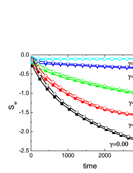
that is a more appropriate form for numerical purposes. Fig. (7) presents the evolution of the Theil entropy for different initial conditions and values of $\gamma$. Except for $\gamma=1$, $\frac{\mbox{d}S_{W}}{\mbox{d}t}<0$ for all times. This implies a different second law for the exchanges defined above. This second law where the entropy decreases instead of increasing characterizes the wealth concentration process (or condensation) and it is the opposite of the “equipartition of energy” obtained in the kinetic theory of gases. This point will be discussed in detail below and we will try to built possible physical systems with a similar behavior.

Figure 7: Time evolution of the entropy for different values of $\gamma$ and two different initial conditions.

If the second law of thermodynamics, when applied to the whole universe, has as a corollary the “thermal death of the universe”, the concentration - or condensation - of wealth leads to a “thermal death of the market”, since the market needs exchanges, or flux of capital, to survive. If all agents, with a few exceptions, have zero wealth, there is almost no exchanges. This can be verified if we calculate the “liquidity”, or the money being exchanged in the system. We define the liquidity of the market as the amount of money exchanged per unit time:

$$C(t)=\frac{1}{2}\int_{0}^{\infty}dw^{\prime}\int_{0}^{\infty}dw^{\prime\prime}N(w^{\prime},t)N(w^{\prime\prime},t)\frac{w^{\prime}w^{\prime\prime}}{w^{\prime}+w^{\prime\prime}}$$ (16)

The liquidity has been numerically calculated for different times and it is represented in Fig. 8. The liquidity is also a decreasing function of time for $\gamma<1$.

Figure 8: Evolution of exchanged wealth for different initial conditions and values of $\gamma$. It is possible to observe that it decreases in time, leading to a thermal death of the market

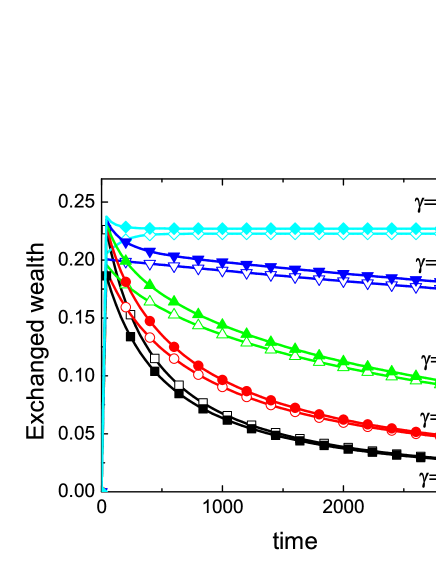
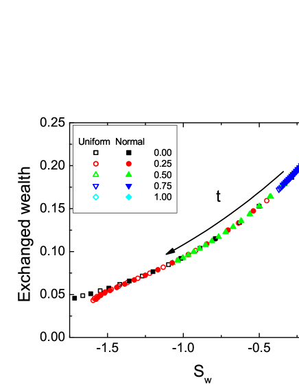
One can argue that this behavior of the $W$-entropy and of the liquidity are artifacts because we have considered a wealth conserving system, and this is not realistic. However, within a very simplified description of the wealth generation process one can expect that the wealth production should be proportional to the circulating capital: wealth must be exchanged to generate more wealth. (Adam Smith said that trade and exchange are emblematic of the nature of men: “Nobody ever saw a dog make a fair and deliberate exchange of one bone for another with another dog.” [33]) In this case it is interesting to investigate the dependence of the total exchanged wealth, $C(t)$, with the wealth distribution. Wealth concentration is supposed to decrease with $W$-entropy $S_{W}$, then, we represented in Fig. 9 $C$ versus $S_{W}$ for all times and for both initial conditions. The circulating capital is an increasing function of $S_{W}$, which means that the more concentrated the wealth is, the smaller wealth production should be expected, confirming that even for a non-conservative market this alternative second law is still valid.

Figure 9: The liquidity, or circulating capital, $C$, as function of the wealth entropy $S_{W}$ for different initial conditions and values of $\gamma$. $C$ increases with $S_{W}$, showing that evenly distributed wealth leads to higher wealth exchanges.

4.2 Why the market condenses?

We focus now on the characteristics of the dynamics that explain condensation as the attractor of the evolution equation. The first reason is that the state of total misery, that is, agents with $w=0$, is a trapping state with zero escaping probability. The second point is that, regardless an agent wealth, the probability that eventually it approaches $w=0$ is non-null. On the other hand, as wealth is conserved, the accumulation of agents near $w=0$ implies few agents with very large $w$. To further illustrate this point, we calculated the average probability $Q_{+}(w)$ for an agent with wealth $w$ to increase its wealth in a given time step, as

$$Q_{+}(w) = \int_{0}^{\infty}dw^{\prime}\,N(w^{\prime},t)p_{\gamma}(w|w^{\prime})$$ (17)

$$= \frac{1-\gamma<\tanh(w-w^{\prime})>}{2}$$

where $<...>$ stands for the average over $N(w^{\prime},t)$. Assume a wealth distribution peaked around $<w>$. For $w$ much lower than the typical values in the wealth distribution, $\tanh(w^{\prime}-w)$ approaches $-1$ when $N(w^{\prime},t)>0$ and hence $Q_{+}(w)\sim\frac{1+\gamma}{2}$. If $\gamma<1$ there is a non zero probability for the agent to loose in a transaction and of approaching the total misery state. This total misery state is a financial hell, as once there, in the words of Dante: Lasciate ogni speranza, voi che entrate, i.e. there are no chances to escape. The wealth distribution will approach the condensate ‘L’-shape configuration. Only for $\gamma=1$ the dynamics guarantees that the probability of loosing wealth is zero for the poorest. This is the one case where the ’L’-solution is not the attractor of the dynamics. The stationary regime in this model and the condition of conservation of the total wealth implies that there are a few infinitely rich agents, since there is not a bound in the maximum possible wealth. As wealth is conserved that implies many poor agents, and a very unfair wealth distribution.

4.3 Lorenz curves and Gini coefficient

In the previous section we have defined the $W$-entropy or Theil coefficient. Another useful and current measure of inequality is the Gini coefficient [31]. To evaluate this coefficient, we first construct the Lorenz curves by defining $x(w_{Z})$ as the fraction of the agent population with wealth lower or equal to $w_{Z}$, that is,

$$x(w_{Z})=\int_{0}^{w_{Z}}N(w,t)dw,$$ (18)

and the fraction of wealth $F(w_{Z})$ belonging to this population as

$$F(w_{Z})=\int_{0}^{w_{Z}}N(w,t)\frac{w}{\langle w\rangle}dw$$ (19)

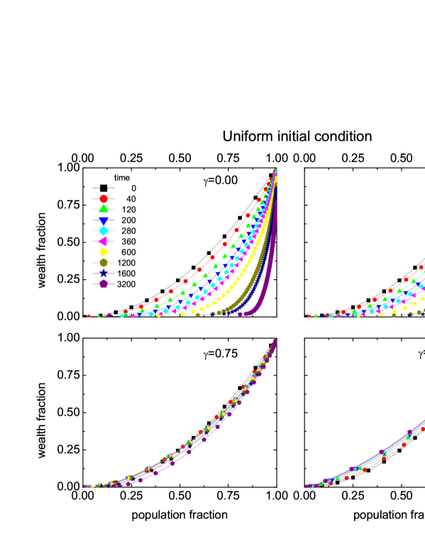
As both $x(w_{Z})$ and $F(w_{Z})$ are uniquely defined by $w_{Z}$ we may build a function $L(x)$, called the Lorenz curve, as the fraction of wealth $F(w_{Z})$ calculated at a value of $w_{Z}$ that corresponds to the population fraction $x$. Fig. 10 shows the time evolution of the Lorenz curves corresponding to the runs with uniform initial conditions. It is clear from the figure that the Lorenz curves present a negative curvature whose absolute value increases in time for $\gamma<1$ and, as one should expect, the limit for $t\rightarrow\infty$ is a condensed state, or an almost $L$-distribution for zero or a small value of $\gamma$, while the share of the wealth is rather stable and even improves for high values of $\gamma$.

Figure 10: Lorenz curves as a function of time for different values of $\gamma$, at different times

The Gini coefficient is defined as [31]

$$G=1-2\int_{0}^{1}L(x)dx$$ (20)

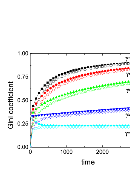
which gives a measure of how unequal the wealth distribution is: for a distribution where all agents have the same amount of wealth, $N(w,t)=\delta(w-\langle w\rangle)$, the Lorenz curve is a straight line such that $\int_{0}^{1}L(x)dx=0.5$, yielding $G=0$. On the other hand when all wealth belong to just one agent, $G=1$. Fig.  11 shows the evolution of the Gini coefficient for the iterations starting from a normal distribution and from a uniform distribution. The initial value of the Gini coefficient is higher in the case of the uniform distribution but for $t\simeq 1000$ time steps the system already “forgot” the initial conditions and the Gini coefficient monotonically increases asymptotically approaching $1$ for $t\rightarrow\infty$.

Figure 11: Time evolution of the Gini coefficient. Note that, after a short transient, the Gini coefficient is a monotonically increasing function of time when $\gamma<1$.

5 Discussion and Conclusion

We have shown, both by analytical and numerical methods that exchange models where the exchange fraction cannot be bigger than the capital of any of the participants, leads to a condensed state and so, to a state of minimum entropy, in disagreement with the second law of thermodynamics. However, this state is a state of equilibrium and a state that represents a kind of thermal dead of markets, as no more exchanges are possible when all, or almost all agents (with the exception of a set of zero measure), have wealth equal to zero. That means that this kind of exchange rule induces a behavior completely different of the one predicted by Boltzmann H-theorem. The main difference comes from the quantity of wealth, (or of the exchanged resource), that the agents can exchange. As we discussed previously, if the exchange assets are determined completely at random, the Boltzmann-Gibbs distribution is recovered [9]. Also, if an “unfair” rule of exchange is introduced, for instance allowing one agent to take all the assets of the other partner, a distribution with a higher Gini coefficient is obtained and there is no condensed state [30, 14].

Thus, it seems that condensation emerges from the fact that it is impossible to receive more money that the quantity already owned. What seems to be a fair exchange rule has the implication of spreading misery. To avoid condensation and the thermal death of markets some regulation, or some minimum allowance is necessary to favor the poorer agents. When there are no regulations and/or when no one can win more than he has, the dynamics leads to a condensed state and to a frozen economy. This result emphasize the importance of regulations and also of loans, as they permit to invest more capital than the one owned by each agent. Also, politics of acting on the poorest agent, as described in an extremal dynamics model [19], tend to avoid this condensed state.

If one wants to compare this result with the second law of thermodynamics applied to physical systems, or to thermodynamic models for economic systems as the ones described, for example, by Mimkes [35] then random or unfair exchanges are essential features to recover the second law. This effect may seem awkward but we can think of physical systems where the exchange rule is similar to the one proposed here and, indeed, there exist physical systems that behave in a similar way. Maybe the best known example are the moderators used in nuclear reactors, where particular materials are used to thermalize neutrons transforming a wide distribution of energy into a distribution with a pronounced peak in the region of energy of interest. One can argue that even if the entropy of the neutrons decreases, the total entropy of the system increases. That is a good clue to better understand the behavior of the exchange model for markets. If the studied exchange model leads to a decrease of entropy and then to an ordered state of minimum entropy, this is because a) each agent is described by a single parameter, his wealth, and b) because poor agents have no possibility of recovery. This last item is important when considering policies to improve the wealth distribution. Concerning the first item we should be aware that a pure exchange models provides a limited description of markets and trade, as they do not consider neither regulatory policies, nor production of goods and commodities, nor salaries, nor banks, nor debts. The limitation of those models was extensively discussed by Gallegati et. al. [34]. Nevertheless, in spite of their simplicity, we think that exchange models capture an essential characteristic of economical activity, and, in particular, of markets, i.e. accumulation of wealth in a few hands, on the other hand they show that equilibrium is probably not an essential ingredient in the description of markets. However, in the same way that uniform temperature leads a physical system to thermal death, in economic systems the thermal death is a consequence of a extreme inequality in revenues and wealth, and we hope to have exhaustively demonstrated this point in this article.

References

- [1] L.E. Reichl, A Modern Course in Statistical Physics, 2nd. ed., Wiley, New York, 1998
- [2] P. Bak, How Nature Works, Springer-Verlag, New York, 1999
- [3] A. Mas-Collel, M.D. Whiston, J.R. Green J.R., Microeconomic Theory, Oxford University Press, New York, 1995.
- [4] V. Pareto, Cours d’Economie Politique, Vol. 2, F. Pichou, Lausanne, 1897
- [5] H. Aoyama, W. Souma, Y. Fujiwara, Growth and fluctuations of personal and company’s income, Physica A 324 (2003) 352-358
- [6] M. Nirei, W. Souma, Two factor model of income distribution dynamics, Rev. Income Wealth 53 (2000) 440–459
- [7] F. Clementi, M. Gallegati, Power law tails in the Italian personal income distribution, Physica A 350 (2005) 427-438
- [8] S. Sinha, Evidence for power-law tail of the wealth distribution in India, Physica A 359 (2006) 555-562
- [9] A. Dragulescu, V.M. Yakovenko, Statistical mechanics of money, The European J. of Physics B 17 (2000) 723-729
- [10] A. Dragulescu, V.M. Yakovenko, Evidence for the exponential distribution of income in the USA’, The European J. of Physics B 20 (2001) 585-589
- [11] A. Dragulescu V.M. Yakovenko, Exponential and power-law probability distributions of wealth and income in the United Kingdom and the United States, Physica A 299 (2001) 213-221
- [12] V.M. Yakovenko, J. Barkley Rosser, Jr., Colloquium: Statistical mechanics of money, wealth and income, Rev. Mod. Phys. 81 (2009) 1703-1725
- [13] A. Chaterjee, S. Yarlagadda, B.K. Chakrabarti, eds. Econophysics of Wealth Distributions, Springer, Milano, 2005
- [14] G.M. Caon, S. Gonçalves, J.R. Iglesias, The unfair consequences of equal opportunities: Comparing exchange models of wealth distribution, The European Physical Journal - Special Topics, 143 (2007) 69-74
- [15] J. Angle, The surplus theory of social stratification and the size distribution of personal wealth, Soc. Forces 65 (1986) 293– 326
- [16] J. Angle, Deriving the size distribution of personal wealth from ‘the rich get richer, the poor get poorer’, J. Math. Sociol. 18 (1993) 27–46.
- [17] A. Chakraborti, B.K. Charkrabarti, Statistical mechanics of money: how saving propensity affects its distribution’, The European J. of Physics B 17 (2000) 167-170
- [18] S. Pianegonda, J.R. Iglesias, G. Abramson, J.L. Vega, Wealth redistribution with conservative exchanges, Physica A 322 (2003) 667-675
- [19] S. Pianegonda, J.R. Iglesias, Inequalities of wealth distribution in a conservative economy, Physica A 342 (2004) 193-199
- [20] S. Sinha, Stochastic Maps, Wealth Distribution in Random Asset Exchange Models and the Marginal Utility of Relative Wealth, Physica Scripta T 106 (2003) 59-64
- [21] A. Chatterjee, B.K. Chakrabarti, S.S. Manna, Pareto law in a kinetic model of market with random saving propensity, Physica A 335 (2004) 155-163
- [22] B.K. Chakrabarti, A. Chatterjee, Ideal Gas-Like Distributions in Economics: Effects of Saving Propensity, in “Applications of Econophysics”, Ed. H. Takayasu, Conference proceedings of Second Nikkei Symposium on Econophysics, Tokyo, Japan, by Springer-Verlag, Tokyo, 2002. Pages 280-285
- [23] J.R. Iglesias, S. Gonçalves, S. Pianegonda, J.L. Vega, G. Abramson, Wealth redistribution in our small world, Physica A 327 (2003) 12-17
- [24] J.R. Iglesias, S. Gonçalves, G. Abramson, J.L. Vega, Correlation between risk aversion and wealth distribution, Physica A 342 (2004) 186-192
- [25] J.-P. Bouchaud, M. Mézard, Wealth condensation in a simple model of economy, Physica A 282 (2000) 536-545
- [26] C.F. Mourkazel, S. Gonçalves, J.R. Iglesias, M. Achach, R. Huerta, Wealth condensation in a multiplicative random asset exchange model, The European Physical Journal - Special Topics, 143 (2007) 75-79
- [27] N. Scafetta, S. Picozzi, B.J. West, A trade-investment model for distribution of wealth, Physica D 193 (2004) 338–352.
- [28] M. Ausloos, A. P ekalski, Model of wealth and goods dynamics in a closed market, Physica A 373 (2007) 560-568
- [29] J.R. Iglesias, How simple regulations can greatly reduce inequality, Science and Culture (India) 76 (2010) 437-443
- [30] B. Hayes, Follow the money, American Scientist 90 (2002) 400-405
- [31] http://en.wikipedia.org/wiki/Gini_coefficient
- [32] http://en.wikipedia.org/wiki/Theil_index
- [33] Adam Smith, An Inquiry into the Nature And Causes of the Wealth of Nations, Online edition ©1995-2005 Adam Smith Institute, 1776 http://www.adamsmith.org/smith/won/won-b1-c2.html
- [34] M. Gallegati, S. Kee, T. Lux, P. Ormerod, Worrying trends in econophysics, Physica A 370 (2006) 1-6
- [35] J. Mimkes, Y. Aruka, Carnot Process of Wealth Distribution, in Econophysics of Wealth Distributions, A. Chaterjee, S. Yarlagadda and B.K. Chakrabarti, eds. Springer, Milano, 2005