Conjugate Variables as a Resource in Signal and Image Processing

Michael Nölle and Martin Suda

AIT–Austrian Institute of Technology
Safety & Security Department
Optical Quantum Technologies
Abstract.

In this paper we develop a new technique to model joint distributions of signals. Our technique is based on quantum mechanical conjugate variables. We show that the transition probability of quantum states leads to a distance function on the signals. This distance function obeys the triangle inequality on all quantum states and becomes a metric on pure quantum states. Treating signals as conjugate variables allows us to create a new approach to segment them.

Keywords: Quantum information, transition probability, Euclidean distance, Fubini-study metric, Bhattacharyya coefficients, conjugate variable, signal/sensor fusion, signal and image segmentation.

We would like to thank Jozef Gruska and Matthias Jakob for all the valuable discussions as well as Ian Glendinning and Janice Knight for editing the manuscript and the discussions thereabout. We also want to thank our company, the AIT, that enabled this research and the tax payers in Austria who payed for it. Last but not least we thank the reviewers who declined our project proposals on the subject and those who fostered it (to no avail) as they prompted us to show the value in this research even harder.

1. Introduction

Quantum information theory and application areas based upon it, such as quantum computing or quantum cryptography have attracted a massive research interest and are developing rapidly. Quantum computing and quantum cryptography are primarily concerned with the impact that the nature of physical quantum systems has on the respective fields of computing and cryptography. Using physical systems, one has to obey the restrictions imposed by nature on physical quantum states, for example that they are not directly observable. They can be measured, but in general a measurement only reveals parts of the information contained in the quantum state.

Some authors have applied quantum information theory to statistics and probability theory ([3, 4]) as well as signal and image processing applications ([5, 8]). Their work focuses mainly on the abstract mathematical concept of quantum information theory and might be referred to as Quantum Information processing Algorithms (QIA) in analogy to the term Quantum Signal Processing created by Eldar ([8]). Applying the formalism of quantum information theory to information processing on classical computers can result in novel but still ’classical’ algorithms.

In this paper we follow the QIA approach, motivated by the fact that we have found considerably easier descriptions of well suited algorithmic solutions for the problems at hand in several application areas ([20, 23, 21]) within the mathematical setting of the quantum space. One reason might be that we were forced to think more deeply about the normalization of data and observations and the metrical functions to be used. A crucial factor seems to be the ability to represent some relations between two (or more) sources of information jointly as quantum information, i.e. in a quantum state. In analogy to the behaviour of physical conjugate variables, e.g. position and momentum, which play a fundamental role in quantum mechanics, we term this a conjugate information variable. In essence we refer to two sources of information as being conjugate to each other if they are in a special relation: Whenever one of them becomes highly predictable the other one is either undefined or unpredictable and vice versa.

The special relation between physical observations of conjugate quantities was an important factor in the development of quantum mechanics in the early 20thsuperscript20𝑡20^{th} century. In the quantum mechanical setting, Heisenberg’s uncertainty principle expresses this relation, e.g. between momentum and position. To be more precise, momentum and position are represented as operators in quantum mechanics and they are related to each other by derivatives. Here an exact definition of uncertainty means that these operators do not commute.

Our main justification for using the same mathematical structure, i.e. Hilbert spaces, is that information sources exist, which have a similar conjugate relation. As an illustrative example consider we want to observe two species of birds lets say one is blue the other one green and their chirp is quite distinct but cannot be reliably heard during day time due to background noises which are absent at night. Obviously during the day we use our eyes and at night our ears to distinguish the species. But is there a seamless way to fuse both signals that additionally helps us to distinguish them at sunrise or sunset with higher reliability?

Or more seriously, consider a simple classification task where we want to decide whether parts of a function are locally constant, rising, falling or minimum or maximum. We might want to use the derivatives of the function to achieve this, as we know that when the first derivative becomes zero the entire information on the extreme points of the function relies on the sign of the second (or third…) derivative. On the other hand when the second derivative becomes zero, the information whether we found a point of (rising or falling) inflection or the function is constant at this point depends entirely on the first (or third…) derivative. Again it would be desirable to represent the first and second derivative such that in ’grey areas’ in between the two extremes either one alone (if it is more reliable) or both may contribute to the classification result.

The authors are fully aware that most of the material on theoretical quantum information is already covered elsewhere. In particular we refer to the textbooks of Gruska [12] and Nielsen and Chuang [19]. Nonetheless we find it worthwhile to summarize some of the basic ideas behind quantum information theory in order to help readers who are not too familiar with them and the notation used in this area. We will omit reoccurring references to [12, 19], where most of the material is treated in-depth, and indicate when the result can be found elsewhere. This introduction to quantum information theory is contained in Chapter 2 whereas Chapter 3 analyzes the encoding of information into quantum states. In Chapter 4 we take a closer look on two-dimensional systems. A new approach to signal segmentation is given in Chapter 5. We conclude the paper with some discussion and references to future work (Chapters 6, 7).

The fact that in most parts of this paper we consider random variables and distributions rather than signals reflects the fact that we assume the signals to be normalized. In quantum states/signals the same assumption is usually made.

2. An Introduction to Quantum Information Theory

2.1. Quantum Systems, Quantum States and Qubits

The first postulate of quantum mechanics states that any physical system can be described by a unit vector in an associated complex vector space which is called Hilbert space \mathcal{H}. A given unit vector ψ𝜓\vec{\psi} is called the state of the system. In this paper we restrict ourselves to finite dimensional Hilbert spaces. The simplest non-trivial system is a two-dimensional system with the state space =2superscript2\mathcal{H}=\mathbb{C}^{2}. Such systems are called quantum bits or qubits. In the usual mathematical notation, the state of a qubit can thus be written as the vector

(2.1) ψ=(αβ)=αe^0+βe^1withα,βand|α|2+|β|2=1,formulae-sequence𝜓𝛼𝛽𝛼subscript^𝑒0𝛽subscript^𝑒1with𝛼𝛽andsuperscript𝛼2superscript𝛽21\vec{\psi}=\left(\begin{array}[]{c}\alpha\\ \beta\end{array}\right)=\alpha\,\hat{e}_{0}+\beta\,\hat{e}_{1}\quad\mbox{\rm with}\quad\alpha,\beta\in\mathbb{C}\quad\mbox{\rm and}\quad|\alpha|^{2}+|\beta|^{2}=1,

where the basis vectors e^0subscript^𝑒0\hat{e}_{0} and e^1subscript^𝑒1\hat{e}_{1} are orthonormal unit vectors. In quantum computing, it is customary to use the Dirac (or “bra-ket”) notation: The column “ket”-vectors

(2.2) |0e^0=(10)and|1e^1=(01),formulae-sequenceket0subscript^𝑒010andket1subscript^𝑒101\left|0\right\rangle\equiv\hat{e}_{0}=\left(\begin{array}[]{c}1\\ 0\end{array}\right)\quad\mbox{\rm and}\quad\left|1\right\rangle\equiv\hat{e}_{1}=\left(\begin{array}[]{c}0\\ 1\end{array}\right),

or generally |ie^iket𝑖subscript^𝑒𝑖\left|i\right\rangle\equiv\hat{e}_{i} for higher dimensional cases, form the computational or canonical basis of \mathcal{H} and the above state can be written as a superposition

(2.3) |ψ=α|0+β|1.ket𝜓𝛼ket0𝛽ket1\left|\psi\right\rangle=\alpha\,\left|0\right\rangle+\beta\,\left|1\right\rangle.

The dual “bra”-vector ψ|bra𝜓\left\langle\psi\right| corresponds to the associated row-vector (α,β)superscript𝛼superscript𝛽(\alpha^{*},\beta^{*}) with complex conjugate components, thus

(2.4) ψ|=α0|+β1|.bra𝜓superscript𝛼bra0superscript𝛽bra1\left\langle\psi\right|=\alpha^{*}\,\left\langle 0\right|+\beta^{*}\,\left\langle 1\right|.

The scalar product ψ|χinner-product𝜓𝜒\left\langle\psi|\chi\right\rangle and the outer product |ψχ|ket𝜓bra𝜒\left|\psi\right\rangle\left\langle\chi\right| are thus reduced to matrix multiplications. Any linear operator 𝐀::𝐀\mathbf{A}:\mathcal{H}\rightarrow\mathcal{H} over =nsuperscript𝑛\mathcal{H}=\mathbb{C}^{n} can be written as

(2.5) 𝐀=i,jn1ai,j|ij|.𝐀superscriptsubscript𝑖𝑗𝑛1subscript𝑎𝑖𝑗ket𝑖bra𝑗\mathbf{A}=\sum_{i,j}^{n-1}a_{i,j}\left|i\right\rangle\left\langle j\right|.

For a Hermitian operator 𝐀=𝐀𝐀superscript𝐀\mathbf{A}=\mathbf{A}^{\dagger} holds, where in matrix notation 𝐀superscript𝐀\mathbf{A}^{\dagger} is the transpose of 𝐀𝐀\mathbf{A} with conjugate complex entries. Whenever we omit the index bounds, the sum is from 0,,n10𝑛10,\ldots,n-1, where n𝑛n is the dimension of the considered Hilbert space.

The orthonormality and completeness of the computational basis can be written as

(2.6) i|j=δijandi|ii|=𝕀,formulae-sequenceinner-product𝑖𝑗subscript𝛿𝑖𝑗andsubscript𝑖ket𝑖bra𝑖𝕀\left\langle i|j\right\rangle=\delta_{ij}\quad\mbox{\rm and}\quad\sum_{i}\left|i\right\rangle\left\langle i\right|=\mathbb{I},

where δijsubscript𝛿𝑖𝑗\delta_{ij} denotes the Kronecker delta function and 𝕀𝕀\mathbb{I} is the identity. Table 1 summarizes frequently-used Dirac notation and its meaning.

Notation Description
|ψket𝜓\left|\psi\right\rangle general “ket” vector, e.g. |ψ=(c0,c1,)Tket𝜓superscriptsubscript𝑐0subscript𝑐1𝑇\left|\psi\right\rangle=(c_{0},c_{1},\ldots)^{T}
ψ|bra𝜓\left\langle\psi\right| dual “bra” vector to |ψket𝜓\left|\psi\right\rangle, e.g. ψ|=(c0,c1,)bra𝜓superscriptsubscript𝑐0superscriptsubscript𝑐1\left\langle\psi\right|=(c_{0}^{*},c_{1}^{*},\ldots)
|nket𝑛\left|n\right\rangle nthsuperscript𝑛thn^{\mathrm{th}} basis vector of computational basis N={|0,|1,}𝑁ket0ket1N=\{\left|0\right\rangle,\left|1\right\rangle,\ldots\}
ϕ|ψinner-productitalic-ϕ𝜓\left\langle\phi|\psi\right\rangle inner product of |ϕketitalic-ϕ\left|\phi\right\rangle and |ψket𝜓\left|\psi\right\rangle (scalar)
|ϕψ|ketitalic-ϕbra𝜓\left|\phi\right\rangle\left\langle\psi\right| outer product of |ϕketitalic-ϕ\left|\phi\right\rangle and |ψket𝜓\left|\psi\right\rangle (matrix)
|ϕ|ψketitalic-ϕket𝜓\left|\phi\right\rangle\left|\psi\right\rangle tensor product |ϕ|ψtensor-productketitalic-ϕket𝜓\left|\phi\right\rangle\otimes\left|\psi\right\rangle (vector)
|i,jket𝑖𝑗\left|i,j\right\rangle tensor product |i|jket𝑖ket𝑗\left|i\right\rangle\left|j\right\rangle of the basis vectors |iket𝑖\left|i\right\rangle and |jket𝑗\left|j\right\rangle
Table 1. Dirac (“bra-ket”) Notation

2.2. Measurement, von Neumann Measurement

From a physical point of view any information contained in a quantum state |ψket𝜓\left|\psi\right\rangle can only be accessed via a measurement𝑚𝑒𝑎𝑠𝑢𝑟𝑒𝑚𝑒𝑛𝑡measurement which is described by a set of (hermitian) operators adding up to the identity operator (completeness condition):

(2.7) i=0m1𝐌i=𝕀.superscriptsubscript𝑖0𝑚1subscript𝐌𝑖𝕀\sum_{i=0}^{m-1}\mathbf{M}_{i}=\mathbb{I}.

As a result of a measurement on |ψket𝜓\left|\psi\right\rangle we get an index i{0,,m1}=S𝑖0𝑚1𝑆i\in\{0,\ldots,m-1\}=S with some probability. A standard interpretation of a measurement is that the state |ψket𝜓\left|\psi\right\rangle ‘collapses’ onto the post-measurement state 1p(i)Mi|ψ1𝑝𝑖subscript𝑀𝑖ket𝜓\frac{1}{\sqrt{p(i)}}M_{i}\left|\psi\right\rangle with probability p(i)=ψ|Mi|ψ𝑝𝑖quantum-operator-product𝜓subscript𝑀𝑖𝜓p(i)=\left\langle\psi\right|M_{i}\left|\psi\right\rangle. It should be noted that the idea that the quantum state spontaneously is changed via a measurement has been the subject of much debate ever since it was proposed in the 1950s. We do not want to address this issue, as the material discussed here is unaffected by it. The fact that the only direct information we can gain from a physical quantum system is the outcome i𝑖i of the measurement is undisputed. Reapplying the measurement does not change this result any further. This means in particular that we cannot gain any direct information about the co-ordinates of a quantum state.

However if we are given a large number of ’identical’ quantum states and we measure them one by one, we eventually gain the frequency of each index and after proper normalization the probability information p(i)𝑝𝑖p(i) for all iS𝑖𝑆i\in S. Taking the completeness condition (2.7) into account we see that the probabilities properly add up to one: ψ|(im𝐌i)|ψquantum-operator-product𝜓superscriptsubscript𝑖𝑚subscript𝐌𝑖𝜓\left\langle\psi\right|\left(\sum_{i}^{m}\mathbf{M}_{i}\right)\left|\psi\right\rangle =ψ|𝕀|ψ=1absentquantum-operator-product𝜓𝕀𝜓1=\left\langle\psi\right|\mathbb{I}\left|\psi\right\rangle=1. In slightly different terms we get the probability distribution of a discrete random variable over the given index set P(X=i)=p(i)𝑃𝑋𝑖𝑝𝑖P(X=i)=p(i). The values the random variable can take111the elements of the σ𝜎\sigma algebra. and the index of the measurement operators are in a one to one correspondence. The resulting probability distribution is fixed as soon as we are given the state |ψket𝜓\left|\psi\right\rangle and the set of measurement operators 𝐌={𝐌i=0m1}𝐌superscriptsubscript𝐌𝑖0𝑚1\mathbf{M}=\{\mathbf{M}_{i=0}^{m-1}\}. In the next section we will see that the converse in general is not true. That is, a given probability distribution does not uniquely determine a quantum state and/or a set of measurement operators.

In this paper we will restrict ourselves to a particulary simple form of measurement which is described by projectors, the so-called von Neumann measurement. Given a unit vector |ψket𝜓\left|\psi\right\rangle the projector P onto |ψket𝜓\left|\psi\right\rangle takes the form

(2.8) P=|ψψ|.Pket𝜓bra𝜓\textbf{P}=\left|\psi\right\rangle\left\langle\psi\right|.

Applying P|ψ=|ψψ|ψ=1|ψPket𝜓ket𝜓inner-product𝜓𝜓1ket𝜓\textbf{P}\left|\psi\right\rangle=\left|\psi\right\rangle\left\langle\psi|\psi\right\rangle=1\cdot\left|\psi\right\rangle we see that it projects |ψket𝜓\left|\psi\right\rangle onto itself and any other unit vector |χket𝜒\left|\chi\right\rangle is projected onto: |ψψ|χ=ψ|χ|ψket𝜓inner-product𝜓𝜒inner-product𝜓𝜒ket𝜓\left|\psi\right\rangle\left\langle\psi|\chi\right\rangle=\left\langle\psi|\chi\right\rangle\left|\psi\right\rangle, i.e. in the direction of |ψket𝜓\left|\psi\right\rangle times the scalar ψ|χinner-product𝜓𝜒\left\langle\psi|\chi\right\rangle. If P=𝕀PsuperscriptPbottom𝕀P\textbf{P}^{\bot}=\mathbb{I}-\textbf{P} is the projector onto the orthogonal complement space of P, {P,P}PsuperscriptPbottom\{\textbf{P},\textbf{P}^{\bot}\} forms a measurement. For any state |χket𝜒\left|\chi\right\rangle the probability that it is changed into |ψket𝜓\left|\psi\right\rangle via this measurement is

(2.9) p(|χ|ψ)χ|P|χ=χ|ψψ|χ=|ψ|χ|2,𝑝ket𝜒ket𝜓quantum-operator-product𝜒P𝜒inner-product𝜒𝜓inner-product𝜓𝜒superscriptinner-product𝜓𝜒2p\left(\left|\chi\right\rangle\rightarrow\left|\psi\right\rangle\right)\equiv\left\langle\chi\right|\textbf{P}\left|\chi\right\rangle=\left\langle\chi|\psi\right\rangle\left\langle\psi|\chi\right\rangle=\left|\left\langle\psi|\chi\right\rangle\right|^{2},

whereas

(2.10) χ|P|χ=χ|(𝕀P)|χ=1|ψ|χ|2quantum-operator-product𝜒superscriptPbottom𝜒quantum-operator-product𝜒𝕀P𝜒1superscriptinner-product𝜓𝜒2\left\langle\chi\right|\textbf{P}^{\bot}\left|\chi\right\rangle=\left\langle\chi\right|\left(\mathbb{I}-\textbf{P}\right)\left|\chi\right\rangle=1-\left|\left\langle\psi|\chi\right\rangle\right|^{2}

gives the probability that the post measurement state lies in the orthogonal complement space. p(|χ|ψ)=|ψ|χ|2𝑝ket𝜒ket𝜓superscriptinner-product𝜓𝜒2p\left(\left|\chi\right\rangle\rightarrow\left|\psi\right\rangle\right)=\left|\left\langle\psi|\chi\right\rangle\right|^{2} is called the transition probability. In the next section we will analyze these equations further.

2.3. Operator Space, Density Operator

The quantum state space under consideration is usually called the principal system. The operator space over a principal system is given by all linear mappings of this state space onto itself, i.e. given the state space \mathcal{H} the operator space is =Ltensor-productsubscript𝐿\mathcal{H}\otimes\mathcal{H}=L_{\mathcal{H}}. The inner product in the operator space takes the form of the Hilbert-Schmidt inner product:

(2.11) (A;B)=tr(AB);A,B,formulae-sequenceABtrsuperscriptABABtensor-product\left(\textbf{A};\textbf{B}\right)=\mathrm{tr}\,\left(\textbf{A}^{\dagger}\textbf{B}\right);\quad\textbf{A},\textbf{B}\in\mathcal{H}\otimes\mathcal{H},

where the trace of an operator is the sum of the diagonal elements of the operator written as a matrix. In terms of the Dirac notation the trace of an operator may be written as

(2.12) tr(A)trA\displaystyle\mathrm{tr}\,\left(\textbf{A}\right) =\displaystyle= tr(i,jai,j|ij|)=kk|(i,jai,j|ij|)|ktrsubscript𝑖𝑗subscript𝑎𝑖𝑗ket𝑖bra𝑗subscript𝑘bra𝑘subscript𝑖𝑗subscript𝑎𝑖𝑗ket𝑖bra𝑗ket𝑘\displaystyle\mathrm{tr}\,\left(\sum_{i,j}a_{i,j}\left|i\right\rangle\left\langle j\right|\right)=\sum_{k}\left\langle k\right|\left(\sum_{i,j}a_{i,j}\left|i\right\rangle\left\langle j\right|\right)\left|k\right\rangle
=\displaystyle= knak,k.superscriptsubscript𝑘𝑛subscript𝑎𝑘𝑘\displaystyle\sum_{k}^{n}a_{k,k}.

Equation 2.11 enables us to define a norm on Lsubscript𝐿L_{\mathcal{H}}:

A2superscriptnormA2\displaystyle\|\textbf{A}\|^{2} =\displaystyle= tr(AA)=tr((i,jai,j|ij|)l,mal,m|lm|)𝑡𝑟superscriptAAtrsuperscriptsubscript𝑖𝑗subscript𝑎𝑖𝑗ket𝑖bra𝑗subscript𝑙𝑚subscript𝑎𝑙𝑚ket𝑙bra𝑚\displaystyle tr(\textbf{A}^{\dagger}\textbf{A})=\mathrm{tr}\,\left(\left(\sum_{i,j}a_{i,j}\left|i\right\rangle\left\langle j\right|\right)^{\dagger}\sum_{l,m}a_{l,m}\left|l\right\rangle\left\langle m\right|\right)
=\displaystyle= tr(i,jai,j|ji|l,mal,m|lm|)trsubscript𝑖𝑗subscriptsuperscript𝑎𝑖𝑗ket𝑗quantum-operator-product𝑖subscript𝑙𝑚subscript𝑎𝑙𝑚𝑙bra𝑚\displaystyle\mathrm{tr}\,\left(\sum_{i,j}a^{*}_{i,j}\left|j\right\rangle\left\langle i\right|\sum_{l,m}a_{l,m}\left|l\right\rangle\left\langle m\right|\right)
=\displaystyle= tr(i,j,mai,jai,m|jm|)=i,jai,jai,j.trsubscript𝑖𝑗𝑚subscriptsuperscript𝑎𝑖𝑗subscript𝑎𝑖𝑚ket𝑗bra𝑚subscript𝑖𝑗subscriptsuperscript𝑎𝑖𝑗subscript𝑎𝑖𝑗\displaystyle\mathrm{tr}\,\left(\sum_{i,j,m}a^{*}_{i,j}a_{i,m}\left|j\right\rangle\left\langle m\right|\right)=\sum_{i,j}a^{*}_{i,j}a_{i,j}.
(2.13) AnormA\displaystyle\|\textbf{A}\| =\displaystyle= i,jai,jai,j=i,j|ai,j|2.subscript𝑖𝑗subscriptsuperscript𝑎𝑖𝑗subscript𝑎𝑖𝑗subscript𝑖𝑗superscriptsubscript𝑎𝑖𝑗2\displaystyle\sqrt{\sum_{i,j}a^{*}_{i,j}a_{i,j}}=\sqrt{\sum_{i,j}|a_{i,j}|^{2}}.

(2.13) is called the Frobenius norm or Hilbert-Schmidt norm of Lsubscript𝐿L_{\mathcal{H}}. Consequently, for operators A,BLABsubscript𝐿\textbf{A},\textbf{B}\in L_{\mathcal{H}} we may calculate the Euclidian distance ABnormAB\|\textbf{A}-\textbf{B}\| as:

(2.14) ABnormAB\displaystyle\|\textbf{A}-\textbf{B}\| =\displaystyle= i,j(ai,jbi,j)(ai,jbi,j)=i,j[|ai,j|2+|bi,j|22(ai,jbi,j)]subscript𝑖𝑗subscriptsuperscript𝑎𝑖𝑗subscriptsuperscript𝑏𝑖𝑗subscript𝑎𝑖𝑗subscript𝑏𝑖𝑗subscript𝑖𝑗delimited-[]superscriptsubscript𝑎𝑖𝑗2superscriptsubscript𝑏𝑖𝑗22subscript𝑎𝑖𝑗subscriptsuperscript𝑏𝑖𝑗\displaystyle\sqrt{\sum_{i,j}(a^{*}_{i,j}-b^{*}_{i,j})(a_{i,j}-b_{i,j})}=\sqrt{\sum_{i,j}\left[|a_{i,j}|^{2}+|b_{i,j}|^{2}-2\Re\left(a_{i,j}b^{*}_{i,j}\right)\right]}
=\displaystyle= [A2+B22tr(AB)],delimited-[]superscriptnormA2superscriptnormB22trsuperscriptAB\displaystyle\sqrt{\left[\|\textbf{A}\|^{2}+\|\textbf{B}\|^{2}-2\Re\mathrm{tr}\,\left(\textbf{A}\textbf{B}^{\dagger}\right)\right]},

where \Re gives the real part of a complex number.

Finally we would like to emphasis the well known fact that global phase changes of a state do not affect the expectation value of an operator.

Lemma 2.1 (Global phase invariance of the expectation of linear operators).

Let AL𝐴subscript𝐿A\in L_{\mathcal{H}} be a linear operator. Then the expectation of A𝐴A is invariant with respect to global phase changes, i.e. for any |ψ~=eiφ|ψ~ket𝜓superscript𝑒𝑖𝜑ket𝜓\tilde{\left|\psi\right\rangle}=e^{i\varphi}\left|\psi\right\rangle, πφπ𝜋𝜑𝜋-\pi\leq\varphi\leq\pi, |ψnket𝜓superscript𝑛\left|\psi\right\rangle\in\mathbb{C}^{n}:

ψ|~A|ψ~=ψ|A|ψ.~bra𝜓A~ket𝜓quantum-operator-product𝜓A𝜓\tilde{\left\langle\psi\right|}\textbf{A}\tilde{\left|\psi\right\rangle}=\left\langle\psi\right|\textbf{A}\left|\psi\right\rangle.

This is easily verified by

Proof.

ψ|~A|ψ~=eiφψ|Aeiφ|ψ=eiφ+iφψ|A|ψ=ψ|A|ψ.~bra𝜓A~ket𝜓superscript𝑒𝑖𝜑quantum-operator-product𝜓Asuperscript𝑒𝑖𝜑𝜓superscript𝑒𝑖𝜑𝑖𝜑quantum-operator-product𝜓A𝜓quantum-operator-product𝜓A𝜓\tilde{\left\langle\psi\right|}\textbf{A}\tilde{\left|\psi\right\rangle}=e^{-i\varphi}\left\langle\psi\right|\textbf{A}e^{i\varphi}\left|\psi\right\rangle=e^{-i\varphi+i\varphi}\left\langle\psi\right|\textbf{A}\left|\psi\right\rangle=\left\langle\psi\right|\textbf{A}\left|\psi\right\rangle.

After these general remarks on the operator space we will turn our attention to a special subset of operators, the so called density operators. Lets first consider the single qubit state

(2.15) |+=12|0+12|1.ket12ket012ket1\left|+\right\rangle=\frac{1}{\sqrt{2}}\left|0\right\rangle+\frac{1}{\sqrt{2}}\left|1\right\rangle.

When we measure |+ket\left|+\right\rangle by projectors onto the computational basis {|00|,|11|}ket0bra0ket1bra1\{\left|0\right\rangle\left\langle 0\right|,\left|1\right\rangle\left\langle 1\right|\}, we will find that either of the two possible post-measurement states |0ket0\left|0\right\rangle and |1ket1\left|1\right\rangle are equally likely with a transition probability of p0=p1=12subscript𝑝0subscript𝑝112p_{0}=p_{1}=\frac{1}{2}. So the experiment is equivalent to a classical flip of an unbiased coin and we might be tempted to think that |+ket\left|+\right\rangle in fact describes a state where the system state is unknown which is either |0ket0\left|0\right\rangle or |1ket1\left|1\right\rangle with equal probability.

If, however, we measure via {|++|,||}\{\left|+\right\rangle\left\langle+\right|,\left|-\right\rangle\left\langle-\right|\} with

(2.16) |=12|012|1,ket12ket012ket1\left|-\right\rangle=\frac{1}{\sqrt{2}}\left|0\right\rangle-\frac{1}{\sqrt{2}}\left|1\right\rangle,

on the same state |+ket\left|+\right\rangle, then the outcome is deterministic as |+ket\left|+\right\rangle is an eigenvector of |++|\left|+\right\rangle\left\langle+\right|. Obviously, the non-determinism of a quantum measurement is inherently different from the classical randomness of (un)biased coin flips.

There exists an elegant and consistent way to capture both concepts of randomness: Assuming we know that a quantum system is in one of k𝑘k states |ψiketsubscript𝜓𝑖\left|\psi_{i}\right\rangle with the probabilities pisubscript𝑝𝑖p_{i}, then we can aggregate our knowledge of the state in a (semi) positive density operator

(2.17) ρ=i=1kp(i)|ψiψi|withi=1kp(i)=1.formulae-sequence𝜌superscriptsubscript𝑖1𝑘𝑝𝑖ketsubscript𝜓𝑖brasubscript𝜓𝑖withsuperscriptsubscript𝑖1𝑘𝑝𝑖1\rho=\sum_{i=1}^{k}p(i)\left|\psi_{i}\right\rangle\left\langle\psi_{i}\right|\quad\mbox{\rm with}\quad\sum_{i=1}^{k}p(i)=1.

As the probabilities add up to 1 and by the linearity of the trace, it is assured that trρ=tr(i=1kpi|ψiψi|)=i=1kpitr|ψiψi|=i=1kpi=1tr𝜌trsuperscriptsubscript𝑖1𝑘subscript𝑝𝑖ketsubscript𝜓𝑖brasubscript𝜓𝑖superscriptsubscript𝑖1𝑘subscript𝑝𝑖trketsubscript𝜓𝑖brasubscript𝜓𝑖superscriptsubscript𝑖1𝑘subscript𝑝𝑖1\mathrm{tr}\,\rho=\mathrm{tr}\,\left(\sum_{i=1}^{k}p_{i}\left|\psi_{i}\right\rangle\left\langle\psi_{i}\right|\right)=\sum_{i=1}^{k}p_{i}\mathrm{tr}\,\left|\psi_{i}\right\rangle\left\langle\psi_{i}\right|=\sum_{i=1}^{k}p_{i}=1 where we used Eq. 2.12. If trρ2=1trsuperscript𝜌21\mathrm{tr}\,\rho^{2}=1 then ρ𝜌\rho can be written in the form ρ=|ψψ|𝜌ket𝜓bra𝜓\rho=\left|\psi\right\rangle\left\langle\psi\right| and the system is said to be in a pure state. If trρ2<1trsuperscript𝜌21\mathrm{tr}\,\rho^{2}<1, then ρ𝜌\rho is referred to a mixed state. The transition probability p(ρχ)𝑝𝜌𝜒p(\rho\rightarrow\chi) to reduce ρ𝜌\rho (pure or mixed state) to the pure state ρ=|χχ|superscript𝜌ket𝜒bra𝜒\rho^{\prime}=\left|\chi\right\rangle\left\langle\chi\right| when performing a measurement in a basis containing |χket𝜒\left|\chi\right\rangle is the expectation value

(2.18) p(ρχ)=ρχ=χ|ρ|χ.𝑝𝜌𝜒subscriptdelimited-⟨⟩𝜌𝜒quantum-operator-product𝜒𝜌𝜒p(\rho\rightarrow\chi)={\langle\rho\rangle}_{\chi}=\left\langle\chi\right|\rho\left|\chi\right\rangle.

Note that for pure states, (2.18) is equivalent to (2.9), as we would expect.

There are some properties of density operators that should be mentioned:

  • trρ=1tr𝜌1\mathrm{tr}\,\rho=1 (see above);

  • ρ=ρ𝜌superscript𝜌\rho=\rho^{\dagger}, i.e. density operators are hermitian operators;

  • any density operator has a spectral decomposition, ρ=UDU𝜌superscriptUDU\rho=\textbf{U}\textbf{D}\textbf{U}^{\dagger}, where U is a unitary matrix, i.e. UU=𝕀superscriptUU𝕀\textbf{U}^{\dagger}\textbf{U}=\mathbb{I}, and D is a diagonal matrix with nonnegative real diagonal elements. Therefore, ρ=id(i)|uiui|𝜌subscript𝑖𝑑𝑖ketsubscript𝑢𝑖brasubscript𝑢𝑖\rho=\sum_{i}d(i)\left|u_{i}\right\rangle\left\langle u_{i}\right|, with id(i)=1subscript𝑖𝑑𝑖1\sum_{i}d(i)=1, where |uiketsubscript𝑢𝑖\left|u_{i}\right\rangle is the basis generated by the columns of U𝑈U and disubscript𝑑𝑖d_{i} are the diagonal entries of D𝐷D. The |uiketsubscript𝑢𝑖\left|u_{i}\right\rangle are called the eigenbasis of ρ𝜌\rho;

  • consider two density operators in their eigenbasis representation:
    ρ=ip(i)|ψiψi|𝜌subscript𝑖𝑝𝑖ketsubscript𝜓𝑖brasubscript𝜓𝑖\rho=\sum_{i}p(i)\left|\psi_{i}\right\rangle\left\langle\psi_{i}\right| with ip(i)=1subscript𝑖𝑝𝑖1\sum_{i}p(i)=1 and σ=iq(i)|χiχi|𝜎subscript𝑖𝑞𝑖ketsubscript𝜒𝑖brasubscript𝜒𝑖\sigma=\sum_{i}q(i)\left|\chi_{i}\right\rangle\left\langle\chi_{i}\right| with iq(i)=1subscript𝑖𝑞𝑖1\sum_{i}q(i)=1, then tr(ρσ)=i,jp(i)q(j)|ψi|χj|2.tr𝜌𝜎subscript𝑖𝑗𝑝𝑖𝑞𝑗superscriptinner-productsubscript𝜓𝑖subscript𝜒𝑗2\mathrm{tr}\,\left(\rho\sigma\right)=\sum_{i,j}p(i)q(j)\left|\left\langle\psi_{i}|\chi_{j}\right\rangle\right|^{2}. This implies, as pisubscript𝑝𝑖p_{i}, qjsubscript𝑞𝑗q_{j} and |ψi|χj|2superscriptinner-productsubscript𝜓𝑖subscript𝜒𝑗2\left|\left\langle\psi_{i}|\chi_{j}\right\rangle\right|^{2} are nonnegative and real numbers, that tr(ρσ)=tr(ρσ)tr𝜌𝜎tr𝜌𝜎\mathrm{tr}\,\left(\rho\sigma\right)=\Re\mathrm{tr}\,\left(\rho\sigma\right);

  • 0tr(ρσ)10tr𝜌𝜎10\leq\mathrm{tr}\,\left(\rho\sigma\right)\leq 1. The lower bound follows again from the fact that the sum is over nonnegative and real numbers. To verify the upper bound we substitute |ψi|χj|21superscriptinner-productsubscript𝜓𝑖subscript𝜒𝑗21\left|\left\langle\psi_{i}|\chi_{j}\right\rangle\right|^{2}\leq 1, which gives

    (2.19) 0tr(ρσ)=i,jp(i)q(j)|ψi|χj|2i,jp(i)q(j)=1.0tr𝜌𝜎subscript𝑖𝑗𝑝𝑖𝑞𝑗superscriptinner-productsubscript𝜓𝑖subscript𝜒𝑗2subscript𝑖𝑗𝑝𝑖𝑞𝑗10\leq\mathrm{tr}\,\left(\rho\sigma\right)=\sum_{i,j}p(i)q(j)\left|\left\langle\psi_{i}|\chi_{j}\right\rangle\right|^{2}\leq\sum_{i,j}p(i)q(j)=1.

The minimum error discrimination of mixed quantum states is an interesting and well studied problem. We refer the interested reader to pioneering work of [13, 15] and further results in [9, 14] and the literature cited therein.

3. Encoding classical Information as Quantum Information

In Section 2.2 we have seen that given a set of measurement operators 𝐌={𝐌i=0m1}𝐌superscriptsubscript𝐌𝑖0𝑚1\mathbf{M}=\{\mathbf{M}_{i=0}^{m-1}\} and a quantum system |ψket𝜓\left|\psi\right\rangle uniquely determines a probability distribution P(X=i)=p(i),i=0,,m1formulae-sequence𝑃𝑋𝑖𝑝𝑖𝑖0𝑚1P(X=i)=p(i),i=0,\ldots,m-1. In this section we want to analyze the converse, i.e. given a probability distribution we want to determine quantum states and measurement operators that produce it.

Let us consider a random variable X𝑋X. The set of values X𝑋X can take is given by S𝑆S and for any probability distribution

(3.1) xSp(X=x)=1,p(X=x)0,for all xS.formulae-sequencesubscript𝑥𝑆𝑝𝑋𝑥1𝑝𝑋𝑥0for all xS.\sum_{x\in S}p(X=x)=1,\quad p(X=x)\geq 0,\quad\mbox{\rm for all $x\in S$.}\quad

A given probability distribution may be interpreted as vector from the n=|S|𝑛𝑆n=\left|S\right| dimensional real vector space nsuperscript𝑛\mathbb{R}^{n}. In this case the basis of the space can be indexed by the elements of S𝑆S and |x,xSket𝑥𝑥𝑆\left|x\right\rangle,x\in S denotes a basis vector. In this basis we define p(X)|p(X)=xSp(x)|x𝑝𝑋ket𝑝𝑋subscript𝑥𝑆𝑝𝑥ket𝑥\overrightarrow{p(X)}\equiv\left|p(X)\right\rangle=\sum_{x\in S}p(x)\left|x\right\rangle. Due to the linearity of the normalization condition (3.1) the set of all probability distributions forms a n1𝑛1n-1 dimensional hyper-plane, sometimes called simplex, in this space.

As we would like to make a connection between the set of all probability distributions in nsuperscript𝑛\mathbb{R}^{n} and quantum states from a complex Hilbert space n=superscript𝑛\mathbb{C}^{n}=\mathcal{H}, we formerly introduce complex numbers αφxsubscript𝛼subscript𝜑𝑥\alpha_{\varphi_{x}}\in\mathbb{C} such that

(3.2) p(x)=αφxαφx=|αφx|2.𝑝𝑥superscriptsubscript𝛼subscript𝜑𝑥subscript𝛼subscript𝜑𝑥superscriptsubscript𝛼subscript𝜑𝑥2p(x)=\alpha_{\varphi_{x}}^{*}\alpha_{\varphi_{x}}=|\alpha_{\varphi_{x}}|^{2}.

The choice of αφxsubscript𝛼subscript𝜑𝑥\alpha_{\varphi_{x}} is not unique. Using Euler’s Equation on

αφx=p(x)eiφx=p(x)(cosφx+isinφx),πφxπ,formulae-sequencesubscript𝛼subscript𝜑𝑥𝑝𝑥superscript𝑒𝑖subscript𝜑𝑥𝑝𝑥subscript𝜑𝑥𝑖subscript𝜑𝑥𝜋subscript𝜑𝑥𝜋\alpha_{\varphi_{x}}=\sqrt{p(x)}e^{i\varphi_{x}}=\sqrt{p(x)}(\cos\varphi_{x}+i\sin\varphi_{x}),-\pi\leq\varphi_{x}\leq\pi,

Equation (3.2) can be rewritten as

(3.3) p(x)=αφxαφx𝑝𝑥superscriptsubscript𝛼subscript𝜑𝑥subscript𝛼subscript𝜑𝑥\displaystyle p(x)=\alpha_{\varphi_{x}}^{*}\alpha_{\varphi_{x}} =\displaystyle= p(x)cos2φx+p(x)sin2φx.𝑝𝑥superscript2subscript𝜑𝑥𝑝𝑥superscript2subscript𝜑𝑥\displaystyle p(x)\cos^{2}\varphi_{x}+p(x)\sin^{2}\varphi_{x}.

It is noteworthy that all numbers αφxsubscript𝛼subscript𝜑𝑥\alpha_{\varphi_{x}} fulfilling (3.2) lie on a complex sphere with radius p(x)𝑝𝑥\sqrt{p(x)} as can be verified from (3.3).

Already here we see that encoding probabilities as quantum states requires some more information than only the probability distribution if we want to be able to adress all quantum states222To be more precise: we need to know the meaning of ’p(x)𝑝𝑥-\sqrt{p(x)}’. This cannot be derived from the probability distribution alone. One bit of additional information is required. If this bit of information is available, the complex part insures a smooth transition from p(x)𝑝𝑥\sqrt{p(x)} to p(x)𝑝𝑥-\sqrt{p(x)}, i.e. without changing the probability of |xket𝑥\left|x\right\rangle if measured in the same basis.. If we restrict the encoding onto the real nonnegative square root we gain the same quantum state as described in [11].

Consider the (state) vector |ψnket𝜓superscript𝑛\left|\psi\right\rangle\in\mathbb{C}^{n}:

(3.4) |ψ=xSαφx|x.ket𝜓subscript𝑥𝑆subscript𝛼subscript𝜑𝑥ket𝑥\left|\psi\right\rangle=\sum_{x\in S}\alpha_{\varphi_{x}}\left|x\right\rangle.

The set of all projectors onto basis states, {P|x=|xx|,xS}formulae-sequencesubscriptPket𝑥ket𝑥bra𝑥𝑥𝑆\{\textbf{P}_{\left|x\right\rangle}=\left|x\right\rangle\left\langle x\right|,x\in S\}, taken as measurement operators result in the probability distribution p(X)𝑝𝑋p(X) when |ψket𝜓\left|\psi\right\rangle is measured, and fulfill the completeness condition (2.7).

Using (3.3) and the normalization condition (3.1) we see that |ψket𝜓\left|\psi\right\rangle is a unit vector in nsuperscript𝑛\mathbb{C}^{n}. These unit vectors are related to probability distributions via (3.2) and lie on a complex unit hyper-sphere centered at the origin.

We will call the assignment

(3.5) E(p(X=x),C)αφxE𝑝𝑋𝑥𝐶subscript𝛼subscript𝜑𝑥\emph{{E}}\left(p\left(X=x\right),C\right)\rightarrow\alpha_{\varphi_{x}}

quantum encoding of p(X)𝑝𝑋p(X) with respect to the conjugate information C𝐶C. If we want to decode the probability information of the quantum encoding we have to apply {P|x=|xx|,xS}formulae-sequencesubscriptPket𝑥ket𝑥bra𝑥𝑥𝑆\{\textbf{P}_{\left|x\right\rangle}=\left|x\right\rangle\left\langle x\right|,x\in S\} to |ψket𝜓\left|\psi\right\rangle.

3.1. Distances

When given two probability distributions over the same index set a natural and important question is: how similar or how close are they? The answers to this question can be quite diverse depending on the scientific discipline they have been derived from. Table 2 gives an overview on the more frequently used probability distribution distance measures as they can be found in the literature.

Name Formula Metric
Euclidian distance i(p(i)q(i))2subscript𝑖superscript𝑝𝑖𝑞𝑖2\sqrt{\sum_{i}(p(i)-q(i))^{2}} yes
trace or i|p(i)q(i)|subscript𝑖𝑝𝑖𝑞𝑖\sum_{i}|p(i)-q(i)| yes
variational distance ([17])
relative χ2superscript𝜒2\chi^{2} i(p(i)q(i))22(p(i)+q(i))subscript𝑖superscript𝑝𝑖𝑞𝑖22𝑝𝑖𝑞𝑖\sum_{i}\frac{(p(i)-q(i))^{2}}{2(p(i)+q(i))} χ𝜒\chi yes
relative entropy or Kullback- ip(i)logp(i)q(i)=subscript𝑖𝑝𝑖𝑝𝑖𝑞𝑖absent\sum_{i}p(i)\log\frac{p(i)}{q(i)}= no
Leibler divergence ([16]) H(p)ip(i)logq(i)𝐻𝑝subscript𝑖𝑝𝑖𝑞𝑖-H(p)-\sum_{i}p(i)\log q(i)
Jensen-Shannon divergence or JS(p,q)=𝐽𝑆𝑝𝑞absentJS(p,q)= JS(p,q)𝐽𝑆𝑝𝑞\sqrt{JS(p,q)}
symmetric relative entropy ([17]) H(12(p+q))12(H(p)+H(q))𝐻12𝑝𝑞12𝐻𝑝𝐻𝑞H\left(\frac{1}{2}(p+q)\right)-\frac{1}{2}\left(H(p)+H(q)\right) yes
Bhattacharyya distance ([1, 16]) 1ip(i)q(i)1subscript𝑖𝑝𝑖𝑞𝑖1-\sum_{i}\sqrt{p(i)}\sqrt{q(i)} yes
Table 2. Frequently used probability distribution distance measures. p𝑝p and q𝑞q are probability distributions over the same index set. H(p)=ip(i)logp(i)𝐻𝑝subscript𝑖𝑝𝑖𝑝𝑖H(p)=-\sum_{i}p(i)\log p(i) is the Shannon entropy ([7, 10, 2]).

Likewise we find adapted distance measures for quantum states and/or density operators ([9]). Based on the transition probability of quantum states we may define a distance function:

Lemma 3.1.

Let ρ,σL𝜌𝜎subscript𝐿\rho,\sigma\in L_{\mathcal{H}} be density operators, (trρ=trσ=1tr𝜌tr𝜎1\mathrm{tr}\,\rho=\mathrm{tr}\,\sigma=1). Then the function

D(ρ,σ)=1tr(ρσ)𝐷𝜌𝜎1tr𝜌𝜎D(\rho,\sigma)=\sqrt{1-\mathrm{tr}\,\left(\rho\sigma\right)}

satisfies the following properties:

  1. (1)

    0D(ρ,σ)10𝐷𝜌𝜎10\leq D(\rho,\sigma)\leq 1,

  2. (2)

    D(ρ,σ)=D(σ,ρ)𝐷𝜌𝜎𝐷𝜎𝜌D(\rho,\sigma)=D(\sigma,\rho), (symmetry)

  3. (3)

    for any density operator τL,trτ=1formulae-sequence𝜏subscript𝐿tr𝜏1\tau\in L_{\mathcal{H}},\mathrm{tr}\,\tau=1:

    D(ρ,σ)D(ρ,τ)+D(τ,σ),(triangle inequality)𝐷𝜌𝜎𝐷𝜌𝜏𝐷𝜏𝜎(triangle inequality)D(\rho,\sigma)\leq D(\rho,\tau)+D(\tau,\sigma),\quad\textrm{(triangle inequality)}
  4. (4)

    on pure states D(.,.)D(.,.) defines a metric.

The fact that D𝐷D defines a metric on pure states is well known ([19], p. 500). In the literature it is sometimes called no-name metric and it is closely related to the so called Fubini study metric. Nevertheless, we would like to prove Lemma 3.1 as the proof offers some insight into the relation of D𝐷D and the Euclidian metric of the operator space and the principal system.

Proof.

Property (1) of Lemma 3.1 is a direct consequence of Equation (2.19). Property (2) follows from the fact that the trace of an operator product is invariant against cyclic permutations of the arguments, i.e. tr(ρσ)=tr(σρ)tr𝜌𝜎tr𝜎𝜌\mathrm{tr}\,(\rho\sigma)=\mathrm{tr}\,(\sigma\rho).

Let ρ,σ,τL𝜌𝜎𝜏subscript𝐿\rho,\sigma,\tau\in L_{\mathcal{H}} be density operators, i.e. trρ=trσ=trτ=1tr𝜌tr𝜎tr𝜏1\mathrm{tr}\,\rho=\mathrm{tr}\,\sigma=\mathrm{tr}\,\tau=1 and ρ1,σ1,τ1formulae-sequencenorm𝜌1formulae-sequencenorm𝜎1norm𝜏1\|\rho\|\leq 1,\|\sigma\|\leq 1,\|\tau\|\leq 1. To see property (3) we first note that the Euclidian distance (see Equation 2.11) of the operator space fulfills the triangle inequality for all operators in Lsubscript𝐿L_{\mathcal{H}}, i.e. ρσρτ+τσnorm𝜌𝜎norm𝜌𝜏norm𝜏𝜎\|\rho-\sigma\|\leq\|\rho-\tau\|+\|\tau-\sigma\| holds. We calculate

ρσ2superscriptnorm𝜌𝜎2\displaystyle\|\rho-\sigma\|^{2} \displaystyle\leq (ρτ+τσ)2superscriptnorm𝜌𝜏norm𝜏𝜎2\displaystyle\left(\|\rho-\tau\|+\|\tau-\sigma\|\right)^{2}
ρ2+σ22tr(ρσ)superscriptnorm𝜌2superscriptnorm𝜎22tr𝜌𝜎\displaystyle\|\rho\|^{2}+\|\sigma\|^{2}-2\mathrm{tr}\,\left(\rho\sigma\right) \displaystyle\leq ρτ2+τσ2+2ρττσsuperscriptnorm𝜌𝜏2superscriptnorm𝜏𝜎22norm𝜌𝜏norm𝜏𝜎\displaystyle\|\rho-\tau\|^{2}+\|\tau-\sigma\|^{2}+2\|\rho-\tau\|\|\tau-\sigma\|
=\displaystyle= ρ2+τ22tr(ρτ)+τ2+σ22tr(τσ)+superscriptnorm𝜌2superscriptnorm𝜏22tr𝜌𝜏superscriptnorm𝜏2superscriptnorm𝜎2limit-from2tr𝜏𝜎\displaystyle\|\rho\|^{2}+\|\tau\|^{2}-2\mathrm{tr}\,\left(\rho\tau\right)+\|\tau\|^{2}+\|\sigma\|^{2}-2\mathrm{tr}\,\left(\tau\sigma\right)+
+\displaystyle+ 2ρττσ,2norm𝜌𝜏norm𝜏𝜎\displaystyle 2\|\rho-\tau\|\|\tau-\sigma\|,

where we used Equation 2.14 in the last step. Simplifying and expanding the mixed term gives:

tr(ρσ)tr𝜌𝜎\displaystyle-\mathrm{tr}\,\left(\rho\sigma\right) \displaystyle\leq τ2tr(ρτ)tr(τσ)+superscriptnorm𝜏2tr𝜌𝜏limit-fromtr𝜏𝜎\displaystyle\|\tau\|^{2}-\mathrm{tr}\,\left(\rho\tau\right)-\mathrm{tr}\,\left(\tau\sigma\right)+
+\displaystyle+ [ρ2+τ22tr(ρτ)][τ2+σ22tr(τσ)].delimited-[]superscriptnorm𝜌2superscriptnorm𝜏22tr𝜌𝜏delimited-[]superscriptnorm𝜏2superscriptnorm𝜎22tr𝜏𝜎\displaystyle\sqrt{\left[\|\rho\|^{2}+\|\tau\|^{2}-2\mathrm{tr}\,\left(\rho\tau\right)\right]\left[\|\tau\|^{2}+\|\sigma\|^{2}-2\mathrm{tr}\,\left(\tau\sigma\right)\right]}.

By substituting ρ2+τ22superscriptnorm𝜌2superscriptnorm𝜏22\|\rho\|^{2}+\|\tau\|^{2}\leq 2 and τ2+σ22superscriptnorm𝜏2superscriptnorm𝜎22\|\tau\|^{2}+\|\sigma\|^{2}\leq 2 we get

tr(ρσ)tr𝜌𝜎\displaystyle-\mathrm{tr}\,\left(\rho\sigma\right) \displaystyle\leq τ2tr(ρτ)tr(τσ)+superscriptnorm𝜏2tr𝜌𝜏limit-fromtr𝜏𝜎\displaystyle\|\tau\|^{2}-\mathrm{tr}\,\left(\rho\tau\right)-\mathrm{tr}\,\left(\tau\sigma\right)+
+\displaystyle+ 2(1tr(ρτ))(1tr(τσ)).21tr𝜌𝜏1tr𝜏𝜎\displaystyle 2\sqrt{\left(1-\mathrm{tr}\,\left(\rho\tau\right)\right)\left(1-\mathrm{tr}\,\left(\tau\sigma\right)\right)}.

With this we are ready to prove property (3) of the above Lemma. We substitute τ21superscriptnorm𝜏21\|\tau\|^{2}\leq 1 in (3.1) and add 111 to both sides. Then

D(ρ,σ)2=1tr(ρσ)𝐷superscript𝜌𝜎21tr𝜌𝜎\displaystyle D(\rho,\sigma)^{2}=1-\mathrm{tr}\,\left(\rho\sigma\right) \displaystyle\leq 2tr(ρτ)tr(τσ)+2tr𝜌𝜏limit-fromtr𝜏𝜎\displaystyle 2-\mathrm{tr}\,\left(\rho\tau\right)-\mathrm{tr}\,\left(\tau\sigma\right)+
+\displaystyle+ 2(1tr(ρτ))(1tr(τσ))21tr𝜌𝜏1tr𝜏𝜎\displaystyle 2\sqrt{\left(1-\mathrm{tr}\,\left(\rho\tau\right)\right)\left(1-\mathrm{tr}\,\left(\tau\sigma\right)\right)}
=\displaystyle= (1tr(ρτ)+1tr(τσ))2superscript1tr𝜌𝜏1tr𝜏𝜎2\displaystyle\left(\sqrt{1-\mathrm{tr}\,\left(\rho\tau\right)}+\sqrt{1-\mathrm{tr}\,\left(\tau\sigma\right)}\right)^{2}
=\displaystyle= (D(ρ,τ)+D(τ,σ))2.superscript𝐷𝜌𝜏𝐷𝜏𝜎2\displaystyle\left(D(\rho,\tau)+D(\tau,\sigma)\right)^{2}.

Reading top to bottom we see that the triangle inequality holds for D(.,.)D(.,.) and all ρ,σ,τL𝜌𝜎𝜏subscript𝐿\rho,\sigma,\tau\in L_{\mathcal{H}}:

(3.7) D(ρ,σ)D(ρ,τ)+D(τ,σ).𝐷𝜌𝜎𝐷𝜌𝜏𝐷𝜏𝜎D(\rho,\sigma)\leq D(\rho,\tau)+D(\tau,\sigma).

For property (4) we have to verify that D(ρ,ρ)=0𝐷𝜌𝜌0D(\rho,\rho)=0. This is only true for pure states as in general trρ21trsuperscript𝜌21\mathrm{tr}\,\rho^{2}\leq 1 with equality if and only if ρ𝜌\rho is pure. On the other hand for pure states D(.,.)D(.,.) fulfills all the requirements of a metric. ∎

Indeed, for pure states D𝐷D is identical to the Euclidian norm of the operator space up to a constant factor, which is easy to verify by noting that for any pure state |ψket𝜓\left|\psi\right\rangle and any density operator σ𝜎\sigma the following holds (see. Eq. 2.12):

(3.8) tr(|ψψ|σ)=ψ|σ|ψ.𝑡𝑟ket𝜓bra𝜓𝜎quantum-operator-product𝜓𝜎𝜓tr\left(\left|\psi\right\rangle\left\langle\psi\right|\sigma\right)=\left\langle\psi\right|\sigma\left|\psi\right\rangle.

If σ𝜎\sigma is pure as well, i.e σ=|ξξ|𝜎ket𝜉bra𝜉\sigma=\left|\xi\right\rangle\left\langle\xi\right|, we get tr(|ψψ|σ)=tr(|ψψ|ξξ|)=|ψ|ξ|2𝑡𝑟ket𝜓bra𝜓𝜎𝑡𝑟ket𝜓inner-product𝜓𝜉bra𝜉superscriptinner-product𝜓𝜉2tr\left(\left|\psi\right\rangle\left\langle\psi\right|\sigma\right)=tr\left(\left|\psi\right\rangle\left\langle\psi|\xi\right\rangle\left\langle\xi\right|\right)=\left|\left\langle\psi|\xi\right\rangle\right|^{2}. With this and equation 2.14 the distance computes to |ψψ||ξξ|=21|ψ|ξ|2normket𝜓bra𝜓ket𝜉bra𝜉21superscriptinner-product𝜓𝜉2\|\left|\psi\right\rangle\left\langle\psi\right|-\left|\xi\right\rangle\left\langle\xi\right|\|=\sqrt{2}\sqrt{1-\left|\left\langle\psi|\xi\right\rangle\right|^{2}} and D(|ψψ|,|ξξ|)=1|ψ|ξ|2𝐷ket𝜓bra𝜓ket𝜉bra𝜉1superscriptinner-product𝜓𝜉2D\left(\left|\psi\right\rangle\left\langle\psi\right|,\left|\xi\right\rangle\left\langle\xi\right|\right)=\sqrt{1-\left|\left\langle\psi|\xi\right\rangle\right|^{2}}. For convenience we will write D(|ψ,|ξ)D(|ψψ|,|ξξ|)𝐷ket𝜓ket𝜉𝐷ket𝜓bra𝜓ket𝜉bra𝜉D(\left|\psi\right\rangle,\left|\xi\right\rangle)\equiv D\left(\left|\psi\right\rangle\left\langle\psi\right|,\left|\xi\right\rangle\left\langle\xi\right|\right) for short when dealing with pure states only.

On pure states the no-name metric takes therefore the form

(3.9) D(|ψ,|ξ)=1|ψ|ξ|2,with|ψ=xαφx|x,|ξ=xβχx|x.formulae-sequence𝐷ket𝜓ket𝜉1superscriptinner-product𝜓𝜉2withformulae-sequenceket𝜓subscript𝑥subscript𝛼subscript𝜑𝑥ket𝑥ket𝜉subscript𝑥subscript𝛽subscript𝜒𝑥ket𝑥D(\left|\psi\right\rangle,\left|\xi\right\rangle)=\sqrt{1-|\left\langle\psi|\xi\right\rangle|^{2}},\quad\mbox{\rm with}\quad\left|\psi\right\rangle=\sum_{x}\alpha_{\varphi_{x}}\left|x\right\rangle,\left|\xi\right\rangle=\sum_{x}\beta_{\chi_{x}}\left|x\right\rangle.

One may derive an intuitive geometric argument to compare two state vectors in nsuperscript𝑛\mathbb{C}^{n} (see Section 3.2 and Figure 1). The vectors |ψket𝜓\left|\psi\right\rangle and |ξket𝜉\left|\xi\right\rangle in general span a two-dimensional complex plane and the intersection of this plane with the hyper-sphere generates a complex unit circle. If |ψ=|ξket𝜓ket𝜉\left|\psi\right\rangle=\left|\xi\right\rangle the intersection degenerates into two points.

Remark (a word of care): Given two probability distributions of the same random variable S𝑆S way may construct corresponding (diagonal) density operators by: ρ=xSp(x)|xx|𝜌subscript𝑥𝑆𝑝𝑥ket𝑥bra𝑥\rho=\sum_{x\in S}p(x)\left|x\right\rangle\left\langle x\right|, σ=xSq(x)|xx|𝜎subscript𝑥𝑆𝑞𝑥ket𝑥bra𝑥\sigma=\sum_{x\in S}q(x)\left|x\right\rangle\left\langle x\right|. Their Euclidian operator distance ρσ2=tr(ρ2)+tr(σ2)2tr(ρσ)superscriptnorm𝜌𝜎2𝑡𝑟superscript𝜌2𝑡𝑟superscript𝜎22𝑡𝑟𝜌𝜎\|\rho-\sigma\|^{2}=tr(\rho^{2})+tr(\sigma^{2})-2tr(\rho\sigma) is equal to the Euclidian distance of the probability distributions. But ρσ22(1tr(ρσ))=2D(ρ,σ)2superscriptnorm𝜌𝜎221𝑡𝑟𝜌𝜎2𝐷superscript𝜌𝜎2\|\rho-\sigma\|^{2}\neq 2(1-tr(\rho\sigma))=2D(\rho,\sigma)^{2} unless both distributions are pure, i.e. for both probability distributions there exists one event, lets say xp,xqsubscript𝑥𝑝subscript𝑥𝑞x_{p},x_{q}, such that p(xp)=q(xq)=1𝑝subscript𝑥𝑝𝑞subscript𝑥𝑞1p(x_{p})=q(x_{q})=1.

For the rest of the chapter we will assume pure states only.

3.1.1. Projection, transition probability

Let |ψ=xSαφx|x,αφx=p(x)eiφxformulae-sequenceket𝜓subscript𝑥𝑆subscript𝛼subscript𝜑𝑥ket𝑥subscript𝛼subscript𝜑𝑥𝑝𝑥superscript𝑒𝑖subscript𝜑𝑥\left|\psi\right\rangle=\sum_{x\in S}\alpha_{\varphi_{x}}\left|x\right\rangle,\alpha_{\varphi_{x}}=\sqrt{p(x)}e^{i\varphi_{x}} and |ξ=xSβχx|x,βχx=q(x)eiχxformulae-sequenceket𝜉subscript𝑥𝑆subscript𝛽subscript𝜒𝑥ket𝑥subscript𝛽subscript𝜒𝑥𝑞𝑥superscript𝑒𝑖subscript𝜒𝑥\left|\xi\right\rangle=\sum_{x\in S}\beta_{\chi_{x}}\left|x\right\rangle,\beta_{\chi_{x}}=\sqrt{q(x)}e^{i\chi_{x}}. As we have seen in Section 2.2, Equation (2.8) the projector P onto |ψket𝜓\left|\psi\right\rangle is given by P=|ψψ|Pket𝜓bra𝜓\textbf{P}=\left|\psi\right\rangle\left\langle\psi\right| and the transition probability

p(|ξ|ψ)=ξ|P|ξ=ξ|ψψ|ξ=|ψ|ξ|2𝑝ket𝜉ket𝜓quantum-operator-product𝜉P𝜉inner-product𝜉𝜓inner-product𝜓𝜉superscriptinner-product𝜓𝜉2p\left(\left|\xi\right\rangle\rightarrow\left|\psi\right\rangle\right)=\left\langle\xi\right|\textbf{P}\left|\xi\right\rangle=\left\langle\xi|\psi\right\rangle\left\langle\psi|\xi\right\rangle=|\left\langle\psi|\xi\right\rangle|^{2}

gives the square of the length of the projection of |ξket𝜉\left|\xi\right\rangle onto |ψket𝜓\left|\psi\right\rangle. Substituting γx=φxχxsubscript𝛾𝑥subscript𝜑𝑥subscript𝜒𝑥\gamma_{x}=\varphi_{x}-\chi_{x} and using Euler’s Equation, we get:

(3.10) ξ|ψinner-product𝜉𝜓\displaystyle\left\langle\xi|\psi\right\rangle =\displaystyle= xSp(x)q(x)eiγxsubscript𝑥𝑆𝑝𝑥𝑞𝑥superscript𝑒𝑖subscript𝛾𝑥\displaystyle\sum_{x\in S}\sqrt{p(x)q(x)}e^{i\gamma_{x}}
=\displaystyle= xScosγxp(x)q(x)+ixSsinγxp(x)q(x),subscript𝑥𝑆subscript𝛾𝑥𝑝𝑥𝑞𝑥𝑖subscript𝑥𝑆subscript𝛾𝑥𝑝𝑥𝑞𝑥\displaystyle\sum_{x\in S}\cos\gamma_{x}\sqrt{p(x)q(x)}+i\sum_{x\in S}\sin\gamma_{x}\sqrt{p(x)q(x)},

and finally

(3.11) |ξ|ψ|2superscriptinner-product𝜉𝜓2\displaystyle|\left\langle\xi|\psi\right\rangle|^{2} =\displaystyle= (xScosγxp(x)q(x))2+(xSsinγxp(x)q(x))2superscriptsubscript𝑥𝑆subscript𝛾𝑥𝑝𝑥𝑞𝑥2superscriptsubscript𝑥𝑆subscript𝛾𝑥𝑝𝑥𝑞𝑥2\displaystyle\left(\sum_{x\in S}\cos\gamma_{x}\sqrt{p(x)q(x)}\right)^{2}+\left(\sum_{x\in S}\sin\gamma_{x}\sqrt{p(x)q(x)}\right)^{2}
=\displaystyle= x,yScos(γxγy)p(x)p(y)q(x)q(y),subscript𝑥𝑦𝑆subscript𝛾𝑥subscript𝛾𝑦𝑝𝑥𝑝𝑦𝑞𝑥𝑞𝑦\displaystyle\sum_{x,y\in S}\cos(\gamma_{x}-\gamma_{y})\sqrt{p(x)p(y)q(x)q(y)},
=\displaystyle= xSp(x)q(x)+x,yxScos(γxγy)p(x)p(y)q(x)q(y),subscript𝑥𝑆𝑝𝑥𝑞𝑥subscript𝑥𝑦𝑥𝑆subscript𝛾𝑥subscript𝛾𝑦𝑝𝑥𝑝𝑦𝑞𝑥𝑞𝑦\displaystyle\sum_{x\in S}p(x)q(x)+\sum_{x,y\neq x\in S}\cos(\gamma_{x}-\gamma_{y})\sqrt{p(x)p(y)q(x)q(y)},

where we used cos(γxγy)=cosγxcosγy+sinγxsinγysubscript𝛾𝑥subscript𝛾𝑦subscript𝛾𝑥subscript𝛾𝑦subscript𝛾𝑥subscript𝛾𝑦\cos(\gamma_{x}-\gamma_{y})=\cos\gamma_{x}\cos\gamma_{y}+\sin\gamma_{x}\sin\gamma_{y} and note that all mixed terms (±icosγxsinγyplus-or-minus𝑖subscript𝛾𝑥subscript𝛾𝑦\pm i\cos\gamma_{x}\sin\gamma_{y}\ldots) disappear.

3.1.2. Length, Euclidian distance of the principal system

It is useful to compute the Euclidian distance of the principal system as well in order to compare it with the metric D𝐷D. This is given by the length of the difference |ψ|ξnormket𝜓ket𝜉\left\|\left|\psi\right\rangle-\left|\xi\right\rangle\right\|:

|ψ|ξ2superscriptnormket𝜓ket𝜉2\displaystyle\left\|\left|\psi\right\rangle-\left|\xi\right\rangle\right\|^{2} =\displaystyle= xS(αφxβχx)(αφxβχx)subscript𝑥𝑆superscriptsubscript𝛼subscript𝜑𝑥subscript𝛽subscript𝜒𝑥subscript𝛼subscript𝜑𝑥subscript𝛽subscript𝜒𝑥\displaystyle\sum_{x\in S}(\alpha_{\varphi_{x}}-\beta_{\chi_{x}})^{*}(\alpha_{\varphi_{x}}-\beta_{\chi_{x}})
=\displaystyle= xSp(x)+q(x)p(x)q(x)(eiγx+eiγx)subscript𝑥𝑆𝑝𝑥𝑞𝑥𝑝𝑥𝑞𝑥superscript𝑒𝑖subscript𝛾𝑥superscript𝑒𝑖subscript𝛾𝑥\displaystyle\sum_{x\in S}p(x)+q(x)-\sqrt{p(x)q(x)}(e^{i\gamma_{x}}+e^{-i\gamma_{x}})
=\displaystyle= xSp(x)+q(x)2p(x)q(x)cosγxsubscript𝑥𝑆𝑝𝑥𝑞𝑥2𝑝𝑥𝑞𝑥subscript𝛾𝑥\displaystyle\sum_{x\in S}p(x)+q(x)-2\sqrt{p(x)q(x)}\cos\gamma_{x}

with γx=φxχxsubscript𝛾𝑥subscript𝜑𝑥subscript𝜒𝑥\gamma_{x}=\varphi_{x}-\chi_{x}. Simplifying by using the normalization condition 3.1 and Equation 3.10 we get:

(3.12) |ψ|ξ2superscriptnormket𝜓ket𝜉2\displaystyle\left\|\left|\psi\right\rangle-\left|\xi\right\rangle\right\|^{2} =\displaystyle= 22xScosγxp(x)q(x)=2(1ξ|ψ).22subscript𝑥𝑆subscript𝛾𝑥𝑝𝑥𝑞𝑥21inner-product𝜉𝜓\displaystyle 2-2\sum_{x\in S}\cos\gamma_{x}\sqrt{p(x)q(x)}=2\;\left(1-\Re\left\langle\xi|\psi\right\rangle\right).

3.1.3. Relation between Projection, no-name metric and Euclidian distance of the principal system

Let P=|ψψ|=UDUPket𝜓bra𝜓superscriptUDU\textbf{P}=\left|\psi\right\rangle\left\langle\psi\right|=\textbf{U}^{\dagger}\textbf{DU} be the spectral decomposition of P, where D is a diagonal matrix with non-negative diagonal entries, and U is unitary. Clearly, ψ|P|ψ=1quantum-operator-product𝜓P𝜓1\left\langle\psi\right|\textbf{P}\left|\psi\right\rangle=1 and therefore, U|ψ=|kUket𝜓ket𝑘\textbf{U}\left|\psi\right\rangle=\left|k\right\rangle is a basis vector in some appropriate basis system and D=|kk|Dket𝑘bra𝑘\textbf{D}=\left|k\right\rangle\left\langle k\right|. Define |ξ=U|ξ=jαj|jketsuperscript𝜉Uket𝜉subscript𝑗superscriptsubscript𝛼𝑗ket𝑗\left|\xi^{\prime}\right\rangle=\textbf{U}\left|\xi\right\rangle=\sum_{j}\alpha_{j}^{\prime}\left|j\right\rangle. Then, with αj=aj+ibjsuperscriptsubscript𝛼𝑗subscript𝑎𝑗𝑖subscript𝑏𝑗\alpha_{j}^{\prime}=a_{j}+ib_{j}, a,b𝑎𝑏a,b\in\mathbb{R},

ξ|P|ξ=ξ|UDU|ξ=ξ|kk|ξ=αkαk=ak2+bk2,quantum-operator-product𝜉P𝜉quantum-operator-product𝜉superscriptUDU𝜉inner-productsuperscript𝜉𝑘inner-product𝑘superscript𝜉superscriptsubscript𝛼𝑘superscriptsubscript𝛼𝑘superscriptsubscript𝑎𝑘2superscriptsubscript𝑏𝑘2\left\langle\xi\right|\textbf{P}\left|\xi\right\rangle=\left\langle\xi\right|\textbf{U}^{\dagger}\textbf{DU}\left|\xi\right\rangle=\left\langle\xi^{\prime}|k\right\rangle\left\langle k|\xi^{\prime}\right\rangle=\alpha_{k}^{\prime*}\alpha_{k}^{\prime}=a_{k}^{2}+b_{k}^{2},

or in terms of the no-name metric we get:

D(|ψ,|ξ)2=1ak2bk2.𝐷superscriptket𝜓ket𝜉21superscriptsubscript𝑎𝑘2superscriptsubscript𝑏𝑘2D\left(\left|\psi\right\rangle,\left|\xi\right\rangle\right)^{2}=1-a_{k}^{2}-b_{k}^{2}.

The Euclidian distance computes to (see 3.12):

|ψ|ξ2superscriptnormket𝜓ket𝜉2\displaystyle\left\|\left|\psi\right\rangle-\left|\xi\right\rangle\right\|^{2} =\displaystyle= U|ψU|ξ2=|k|ξ2superscriptnormUket𝜓Uket𝜉2superscriptnormket𝑘ketsuperscript𝜉2\displaystyle\left\|\textbf{U}\left|\psi\right\rangle-\textbf{U}\left|\xi\right\rangle\right\|^{2}=\left\|\left|k\right\rangle-\left|\xi^{\prime}\right\rangle\right\|^{2}
=\displaystyle= 2(1ξ|k)=2(1αk)=2(1ak).21inner-productsuperscript𝜉𝑘21superscriptsubscript𝛼𝑘21subscript𝑎𝑘\displaystyle 2\;\left(1-\Re\left\langle\xi^{\prime}|k\right\rangle\right)=2\;(1-\Re\alpha_{k}^{\prime})=2\;(1-a_{k}).

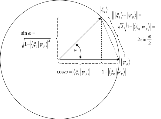
If we assume a real nonnegative principal system this might give some insight into distance functions used in the literature ([1, 22, 6]). In this case as b=0,0a1formulae-sequence𝑏00𝑎1b=0,0\leq a\leq 1 and 1a1a21𝑎1superscript𝑎21-a\leq 1-a^{2} we have (see Fig. 1): D(|ψ,|ξ)|ψ|ξ2D(|ψ,|ξ)𝐷ket𝜓ket𝜉normket𝜓ket𝜉2𝐷ket𝜓ket𝜉D\left(\left|\psi\right\rangle,\left|\xi\right\rangle\right)\leq\left\|\left|\psi\right\rangle-\left|\xi\right\rangle\right\|\leq\sqrt{2}D\left(\left|\psi\right\rangle,\left|\xi\right\rangle\right).

3.2. Dropping the phase

The relation between the Euclidian distance of the principal system and the no-name metric becomes slightly easier (but misleading in general) when we consider no phase information, i.e. when p𝑝p and q𝑞q are represented by their special nonnegative and real choice |ψpketsubscript𝜓𝑝\left|\psi_{{p}}\right\rangle and |ξqketsubscript𝜉𝑞\left|\xi_{{q}}\right\rangle. In this case the complex Hilbert space nsuperscript𝑛\mathbb{C}^{n} is reduced to a real Hilbert space of the same dimension and we may drop the modulus as all probabilities are mapped onto the positive square root. We can visualize the relation of the two measures as can be seen in Figure 1.

The inner product ξq|ψpinner-productsubscript𝜉𝑞subscript𝜓𝑝\left\langle\xi_{{q}}|\psi_{{p}}\right\rangle gives the cosine of the angle between |ψpketsubscript𝜓𝑝\left|\psi_{{p}}\right\rangle and |ξqketsubscript𝜉𝑞\left|\xi_{{q}}\right\rangle and equals the length of the projection of |ξqketsubscript𝜉𝑞\left|\xi_{{q}}\right\rangle onto |ψpketsubscript𝜓𝑝\left|\psi_{{p}}\right\rangle. Likewise 1ξq|ψp21superscriptinner-productsubscript𝜉𝑞subscript𝜓𝑝2\sqrt{1-\left\langle\xi_{{q}}|\psi_{{p}}\right\rangle^{2}} results into the sine of the angle and equals the length of the projection of |ξqketsubscript𝜉𝑞\left|\xi_{{q}}\right\rangle onto the orthogonal complement of |ψpketsubscript𝜓𝑝\left|\psi_{{p}}\right\rangle in the plane spanned by the two state vectors. The length of the difference of the two vectors in terms of the inner product is given by (Eq. 3.12)

(3.13) |ψp|ξq=21ξq|ψp.normketsubscript𝜓𝑝ketsubscript𝜉𝑞21inner-productsubscript𝜉𝑞subscript𝜓𝑝\|\left|\psi_{{p}}\right\rangle-\left|\xi_{{q}}\right\rangle\|=\sqrt{2}\sqrt{1-\left\langle\xi_{{q}}|\psi_{{p}}\right\rangle}.

This relates to a measure between density distributions frequently used in the literature that is based on the so called Bhattacharyya coefficients:

(3.14) d(p(X),q(X))d(p,q)=1xSp(x)q(x)=1ξq|ψp,𝑑𝑝𝑋𝑞𝑋𝑑𝑝𝑞1subscript𝑥𝑆𝑝𝑥𝑞𝑥1inner-productsubscript𝜉𝑞subscript𝜓𝑝d(p(X),q(X))\equiv d(p,q)=\sqrt{1-\sum_{x\in S}\sqrt{p(x)q(x)}}=\sqrt{1-\left\langle\xi_{{q}}|\psi_{{p}}\right\rangle},

which up to a constant factor is equal to (3.13). The sum over the Bhattacharyya coefficients, f(p(X),q(X))=xSp(x)q(x)𝑓𝑝𝑋𝑞𝑋subscript𝑥𝑆𝑝𝑥𝑞𝑥f(p(X),q(X))=\sum_{x\in S}\sqrt{p(x)q(x)}, is usually called the fidelity of the probability distribution p𝑝p and q𝑞q. As an example 3.14 is used in [6] to compare density functions in the context of object tracking.

Let ω𝜔\omega be the angle between |ψpketsubscript𝜓𝑝\left|\psi_{{p}}\right\rangle and |ξqketsubscript𝜉𝑞\left|\xi_{{q}}\right\rangle. Substituting cosω=ξq|ψp𝜔inner-productsubscript𝜉𝑞subscript𝜓𝑝\cos\omega=\left\langle\xi_{{q}}|\psi_{{p}}\right\rangle and observing that sinω2=121cosω𝜔2121𝜔\sin\frac{\omega}{2}=\frac{1}{\sqrt{2}}\sqrt{1-\cos\omega}, we get:

D(p(X),q(X))𝐷𝑝𝑋𝑞𝑋\displaystyle D(p(X),q(X)) =\displaystyle= sinω𝜔\displaystyle\sin\omega
|ψp|ξqnormketsubscript𝜓𝑝ketsubscript𝜉𝑞\displaystyle\|\left|\psi_{{p}}\right\rangle-\left|\xi_{{q}}\right\rangle\| =\displaystyle= 2d(p,q)=2sinω2.2𝑑𝑝𝑞2𝜔2\displaystyle\sqrt{2}d(p,q)=2\sin\frac{\omega}{2}.
Refer to caption
Figure 1. Geometric derivation of several distance measures in nsuperscript𝑛\mathbb{R}^{n}. The intersection of the plane spanned by |ψpketsubscript𝜓𝑝\left|\psi_{{p}}\right\rangle and |ξqketsubscript𝜉𝑞\left|\xi_{{q}}\right\rangle with the unit hypersphere of nsuperscript𝑛\mathbb{R}^{n} generates a unit circle.

For the rest of the paper we will limit our discussion onto two dimensional systems as they allow to be visualized are fairly powerful instruments for concrete applications.

4. Visualization of D𝐷D, the two-dimensional case

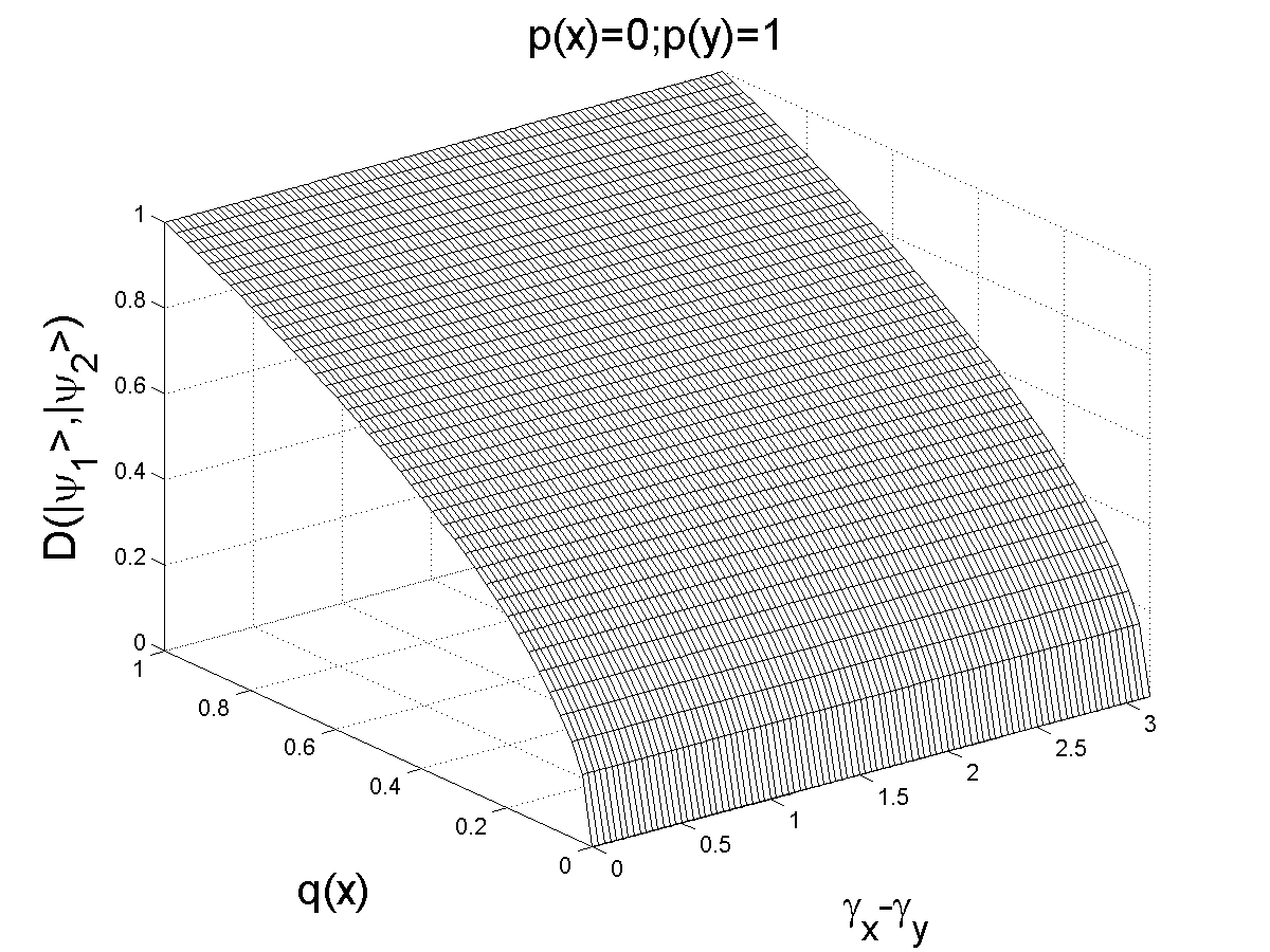
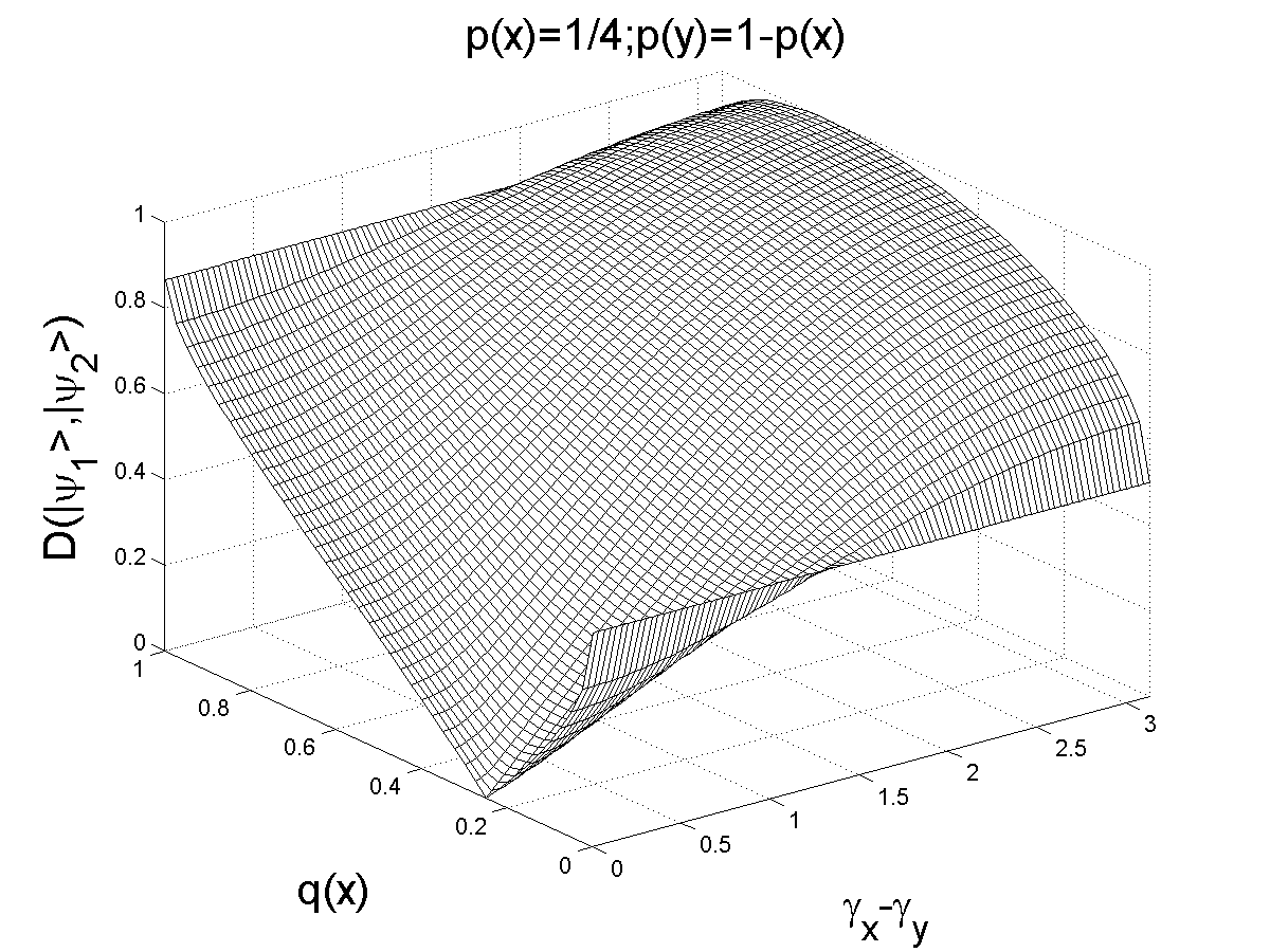
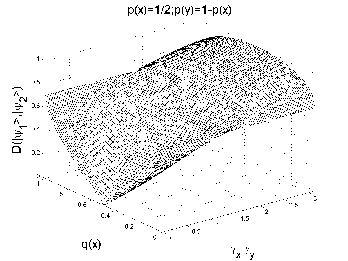
It is worthwhile to study the behavior of the transition probability and the no-name metric more closely. For the two-dimensional Hilbert space 2superscript2\mathbb{C}^{2} and pure states |ψ,|ξ2ket𝜓ket𝜉superscript2\left|\psi\right\rangle,\left|\xi\right\rangle\in\mathbb{C}^{2} we can visualize Equation 3.11 and consequently D(|ψ,|ξ)𝐷ket𝜓ket𝜉D(\left|\psi\right\rangle,\left|\xi\right\rangle).

Refer to caption
Refer to caption
Refer to caption
Refer to caption
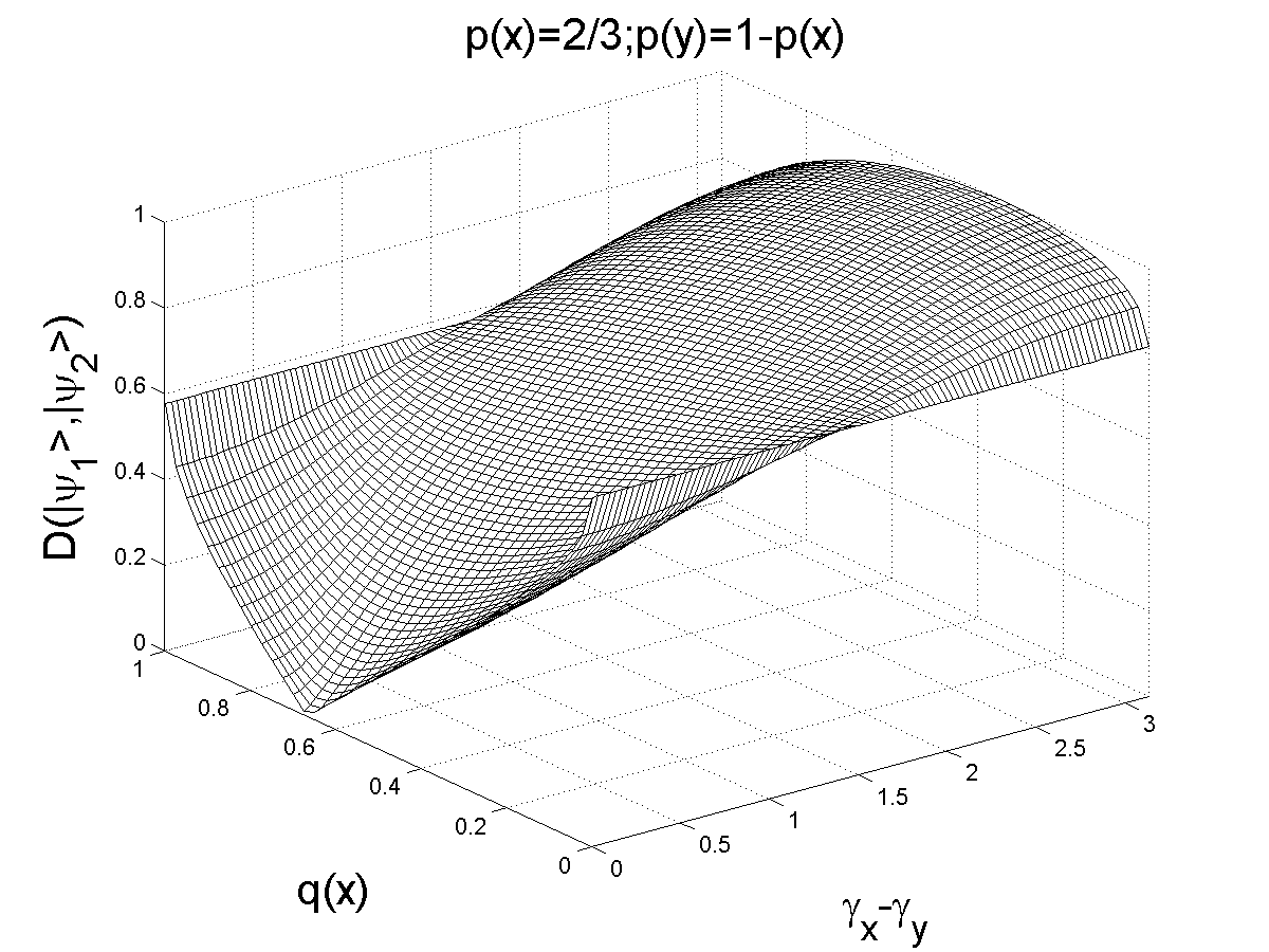
Figure 2. Visualization of D(|ψ,|ξ)𝐷ket𝜓ket𝜉D\left(\left|\psi\right\rangle,\left|\xi\right\rangle\right) for X={x,y}𝑋𝑥𝑦X=\{x,y\} and different values of p𝑝p. q𝑞q ranges over all density distributions and all phase differences between 00 and π𝜋\pi. The range from π𝜋-\pi to 00 is symmetric.
Refer to caption
Refer to caption
Refer to caption
Refer to caption
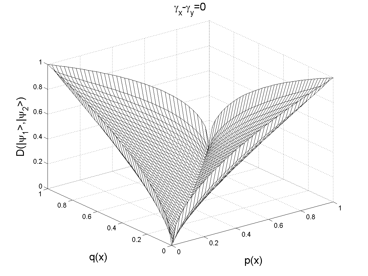
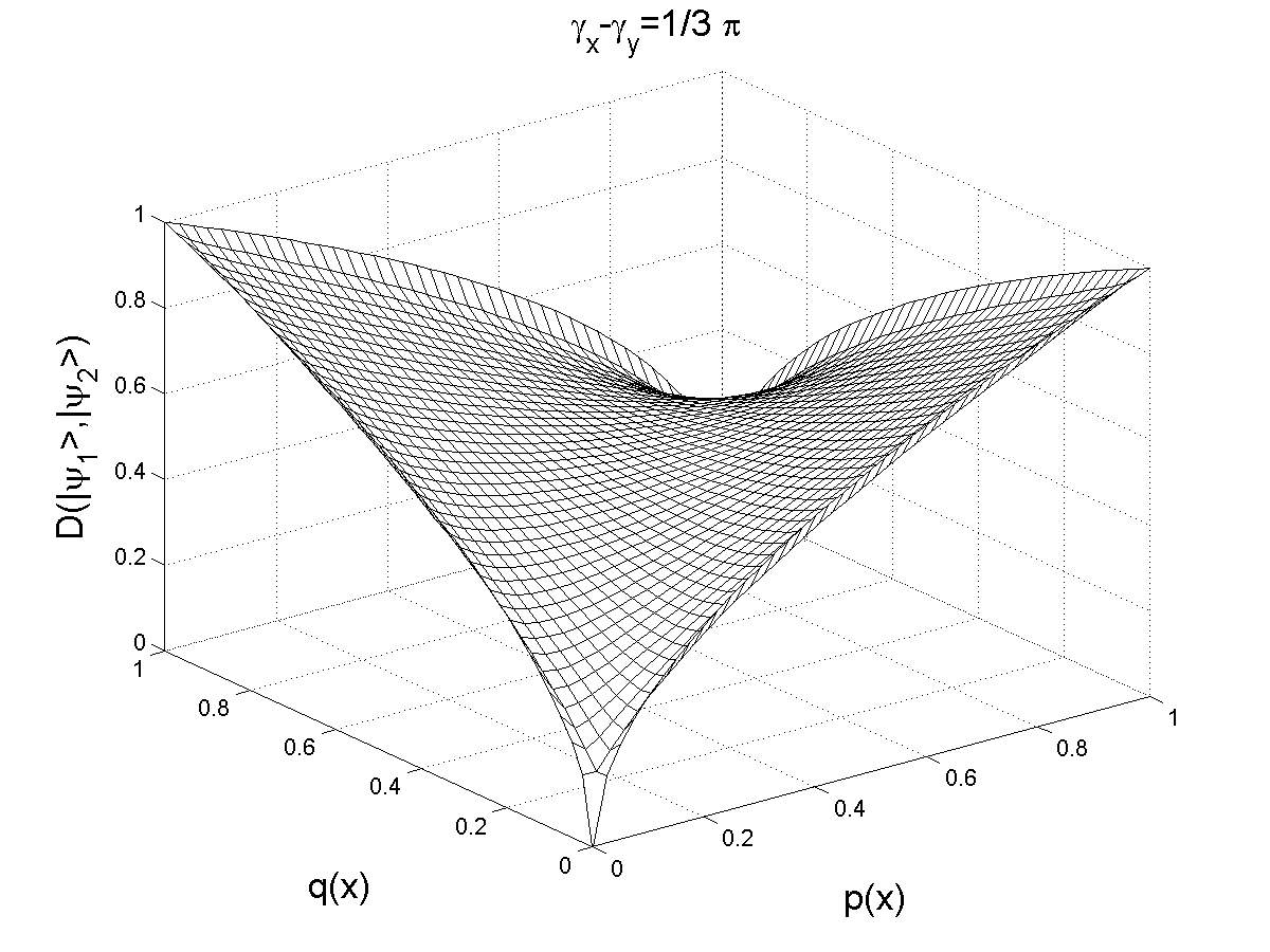
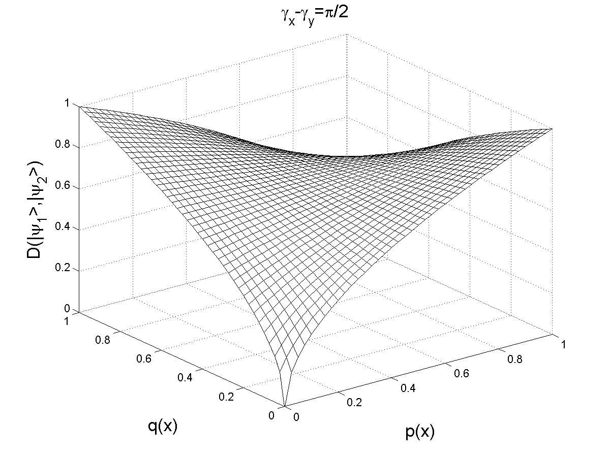
Figure 3. Visualization of D(|ψ,|ξ)𝐷ket𝜓ket𝜉D\left(\left|\psi\right\rangle,\left|\xi\right\rangle\right) for X={x,y}𝑋𝑥𝑦X=\{x,y\} and a fixed phase difference. p𝑝p and q𝑞q range over all possible density distributions.
Refer to caption
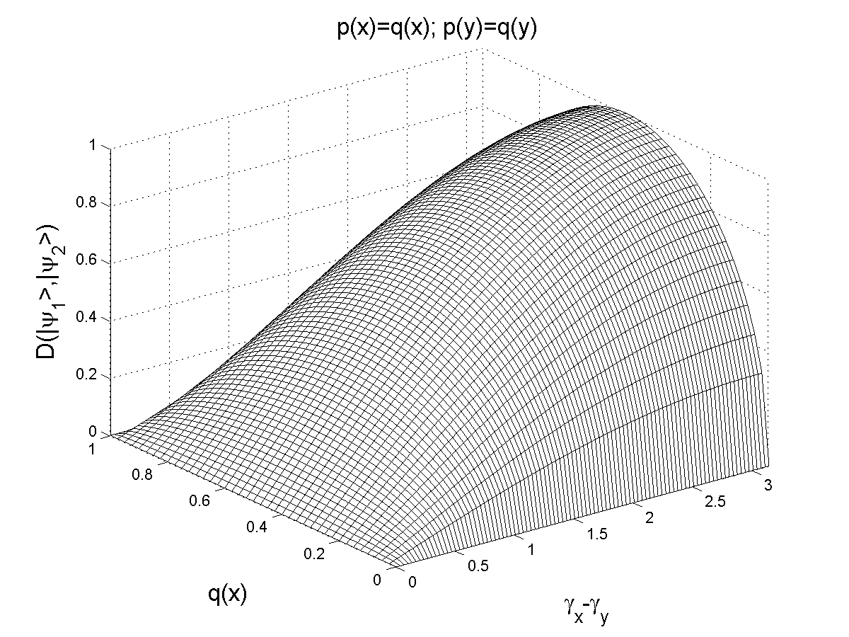
Figure 4. Visualization of D(|ψ,|ξ)𝐷ket𝜓ket𝜉D\left(\left|\psi\right\rangle,\left|\xi\right\rangle\right) for X={x,y}𝑋𝑥𝑦X=\{x,y\} and p=q𝑝𝑞p=q. The phase difference γxγysubscript𝛾𝑥subscript𝛾𝑦\gamma_{x}-\gamma_{y} ranges over all phase differences between 00 and π𝜋\pi. The range from π𝜋-\pi to 00 is symmetric.

Consider density distributions p,q𝑝𝑞p,q over the random variable X={x,y}𝑋𝑥𝑦X=\{x,y\}. In this case the encoding of p𝑝p and q𝑞q as quantum states results in qubits. We want to analyze the impact of the phase factor on the distance of the qubits.

Using Equation 3.11 Equation (3.9) then takes the form

D(|ψ,|ξ)2=1p(x)q(x)p(y)q(y)2cos(γxγy)p(x)p(y)q(x)q(y).𝐷superscriptket𝜓ket𝜉21𝑝𝑥𝑞𝑥𝑝𝑦𝑞𝑦2subscript𝛾𝑥subscript𝛾𝑦𝑝𝑥𝑝𝑦𝑞𝑥𝑞𝑦D\left(\left|\psi\right\rangle,\left|\xi\right\rangle\right)^{2}=1-p(x)q(x)-p(y)q(y)-2\cos(\gamma_{x}-\gamma_{y})\sqrt{p(x)p(y)q(x)q(y)}.

Alternatively, we may express D(|ψ,|ξ)𝐷ket𝜓ket𝜉D\left(\left|\psi\right\rangle,\left|\xi\right\rangle\right) in terms of p(x)=|αx|2𝑝𝑥superscriptsubscript𝛼𝑥2p(x)=|\alpha_{x}|^{2}, p(y)=|αy|2𝑝𝑦superscriptsubscript𝛼𝑦2p(y)=|\alpha_{y}|^{2}, q(x)=|βx|2𝑞𝑥superscriptsubscript𝛽𝑥2q(x)=|\beta_{x}|^{2} and q(y)=|βy|2𝑞𝑦superscriptsubscript𝛽𝑦2q(y)=|\beta_{y}|^{2}:

D(|ψ,|ξ)2=1|αx|2|βx|2|αy|2|βy|22cos(γxγy)|αx||αy||βx||βy|.𝐷superscriptket𝜓ket𝜉21superscriptsubscript𝛼𝑥2superscriptsubscript𝛽𝑥2superscriptsubscript𝛼𝑦2superscriptsubscript𝛽𝑦22subscript𝛾𝑥subscript𝛾𝑦subscript𝛼𝑥subscript𝛼𝑦subscript𝛽𝑥subscript𝛽𝑦D\left(\left|\psi\right\rangle,\left|\xi\right\rangle\right)^{2}=1-|\alpha_{x}|^{2}|\beta_{x}|^{2}-|\alpha_{y}|^{2}|\beta_{y}|^{2}-2\cos(\gamma_{x}-\gamma_{y})|\alpha_{x}||\alpha_{y}||\beta_{x}||\beta_{y}|.
  1. (1)

    Let p𝑝p be fixed and q𝑞q vary over all possible distributions. As p𝑝p is fixed the phase difference γxγysubscript𝛾𝑥subscript𝛾𝑦\gamma_{x}-\gamma_{y} only depends on q𝑞q and we may consider all possible phase differences. A visualization of D(|ψ,|ξ)𝐷ket𝜓ket𝜉D\left(\left|\psi\right\rangle,\left|\xi\right\rangle\right) for several choices of p𝑝p is given in Figure 2.

    1. (a)

      Clearly, D(|ψ,|ξ)=0αx=βx𝐷ket𝜓ket𝜉0subscript𝛼𝑥subscript𝛽𝑥D\left(\left|\psi\right\rangle,\left|\xi\right\rangle\right)=0\Leftrightarrow\alpha_{x}=\beta_{x}, αy=βysubscript𝛼𝑦subscript𝛽𝑦\alpha_{y}=\beta_{y} as then γxγy=0subscript𝛾𝑥subscript𝛾𝑦0\gamma_{x}-\gamma_{y}=0 and

      D(|ψ,|ξ)2=1(|αx|2+|αy|2)2=1(p(x)+p(y))2=0.𝐷superscriptket𝜓ket𝜉21superscriptsuperscriptsubscript𝛼𝑥2superscriptsubscript𝛼𝑦221superscript𝑝𝑥𝑝𝑦20D\left(\left|\psi\right\rangle,\left|\xi\right\rangle\right)^{2}=1-(|\alpha_{x}|^{2}+|\alpha_{y}|^{2})^{2}=1-(p(x)+p(y))^{2}=0.
    2. (b)

      Conversely, D(|ψ,|ξ)=1αx=|βy|ei(χx±π2+η)𝐷ket𝜓ket𝜉1subscript𝛼𝑥subscript𝛽𝑦superscript𝑒𝑖plus-or-minussubscript𝜒𝑥𝜋2𝜂D\left(\left|\psi\right\rangle,\left|\xi\right\rangle\right)=1\Leftrightarrow\alpha_{x}=|\beta_{y}|e^{i(\chi_{x}\pm\frac{\pi}{2}+\eta)},
      αy=|βx|ei(φq,yπ2+η)subscript𝛼𝑦subscript𝛽𝑥superscript𝑒𝑖minus-or-plussubscript𝜑𝑞𝑦𝜋2𝜂\alpha_{y}=|\beta_{x}|e^{i(\varphi_{q,y}\mp\frac{\pi}{2}+\eta)}, η𝜂\eta\in\mathbb{R}, which gives γxγy=±πsubscript𝛾𝑥subscript𝛾𝑦plus-or-minus𝜋\gamma_{x}-\gamma_{y}=\pm\pi, resulting in

      D(|ψ,|ξ)2=1|βy|2|βx|2|βx|2|βy|2+2|βx|2|βy|2=1.𝐷superscriptket𝜓ket𝜉21superscriptsubscript𝛽𝑦2superscriptsubscript𝛽𝑥2superscriptsubscript𝛽𝑥2superscriptsubscript𝛽𝑦22superscriptsubscript𝛽𝑥2superscriptsubscript𝛽𝑦21D\left(\left|\psi\right\rangle,\left|\xi\right\rangle\right)^{2}=1-|\beta_{y}|^{2}|\beta_{x}|^{2}-|\beta_{x}|^{2}|\beta_{y}|^{2}+2|\beta_{x}|^{2}|\beta_{y}|^{2}=1.
  2. (2)

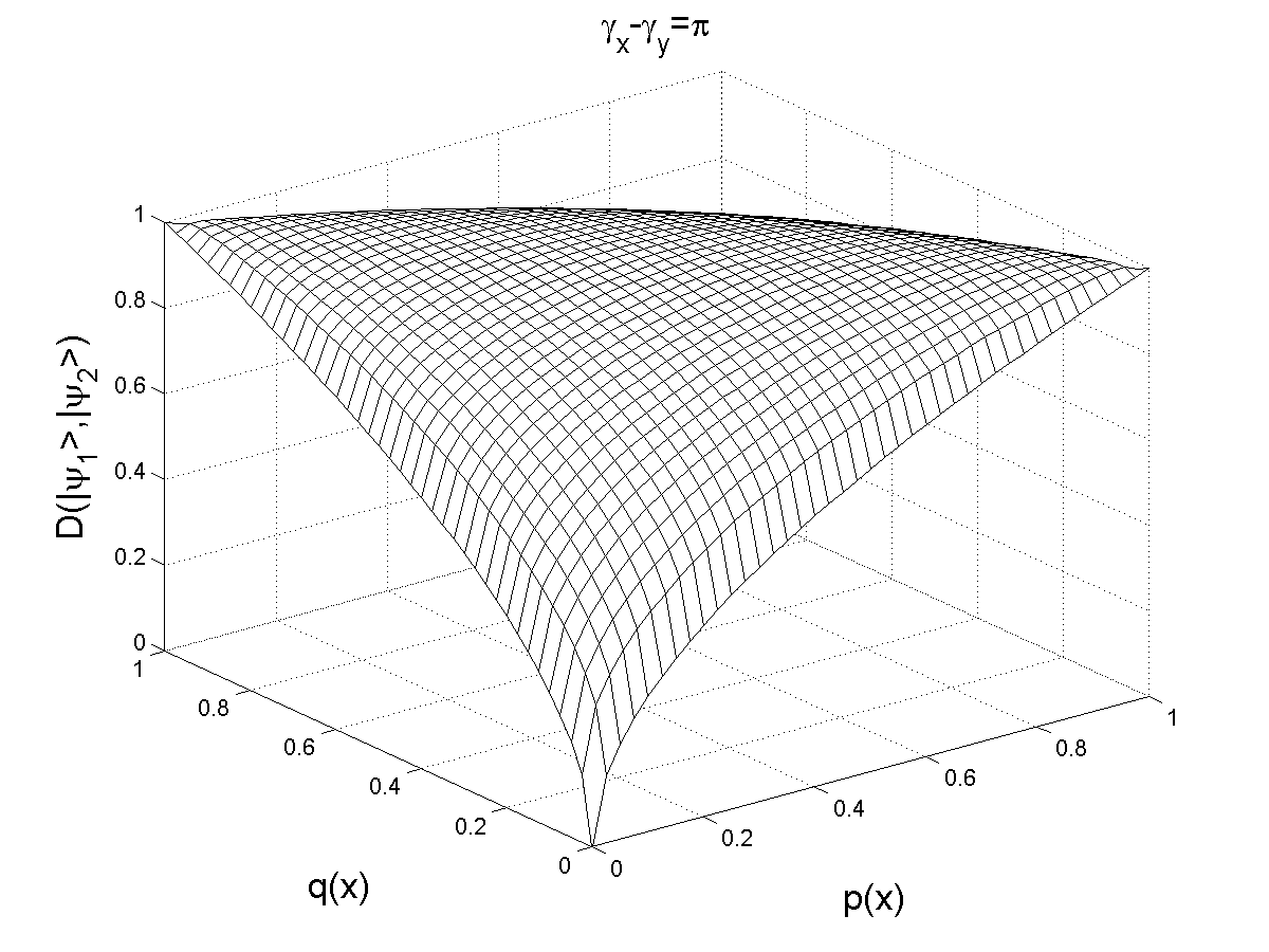
    Now let γxγysubscript𝛾𝑥subscript𝛾𝑦\gamma_{x}-\gamma_{y} be fixed and p,q𝑝𝑞p,q vary over all possible distributions. A visualization of D(|ψ,|ξ)𝐷ket𝜓ket𝜉D\left(\left|\psi\right\rangle,\left|\xi\right\rangle\right) for several choices of γxγysubscript𝛾𝑥subscript𝛾𝑦\gamma_{x}-\gamma_{y} is given in Figure 3.

    1. (a)

      γxγy=0subscript𝛾𝑥subscript𝛾𝑦0\gamma_{x}-\gamma_{y}=0:

      D(|ψ,|ξ)2𝐷superscriptket𝜓ket𝜉2\displaystyle D\left(\left|\psi\right\rangle,\left|\xi\right\rangle\right)^{2} =\displaystyle= 1p(x)q(x)p(y)q(y)2p(x)p(y)q(x)q(y)1𝑝𝑥𝑞𝑥𝑝𝑦𝑞𝑦2𝑝𝑥𝑝𝑦𝑞𝑥𝑞𝑦\displaystyle 1-p(x)q(x)-p(y)q(y)-2\sqrt{p(x)p(y)q(x)q(y)}
      =\displaystyle= 1(p(x)q(x)+p(y)q(y))21superscript𝑝𝑥𝑞𝑥𝑝𝑦𝑞𝑦2\displaystyle 1-\left(\sqrt{p(x)q(x)}+\sqrt{p(y)q(y)}\right)^{2}
      D(|ψ,|ξ)𝐷ket𝜓ket𝜉\displaystyle D\left(\left|\psi\right\rangle,\left|\xi\right\rangle\right) =\displaystyle= 0p(x)=q(x)and0𝑝𝑥𝑞𝑥and\displaystyle 0\Leftrightarrow p(x)=q(x)\quad\mathrm{and}
      D(|ψ,|ξ)𝐷ket𝜓ket𝜉\displaystyle D\left(\left|\psi\right\rangle,\left|\xi\right\rangle\right) =\displaystyle= 1p(x)=q(y)=0p(x)=q(y)=1.1𝑝𝑥𝑞𝑦0𝑝𝑥𝑞𝑦1\displaystyle 1\Leftrightarrow p(x)=q(y)=0\vee p(x)=q(y)=1.

      When p(x)=q(x)𝑝𝑥𝑞𝑥p(x)=q(x) for all xX𝑥𝑋x\in X we have a perfect correlation.

    2. (b)

      γxγy=±π3subscript𝛾𝑥subscript𝛾𝑦plus-or-minus𝜋3\gamma_{x}-\gamma_{y}=\pm\frac{\pi}{3}:

      D(|ψ,|ξ)2𝐷superscriptket𝜓ket𝜉2\displaystyle D\left(\left|\psi\right\rangle,\left|\xi\right\rangle\right)^{2} =\displaystyle= 1p(x)q(x)p(y)q(y)p(x)p(y)q(x)q(y)1𝑝𝑥𝑞𝑥𝑝𝑦𝑞𝑦𝑝𝑥𝑝𝑦𝑞𝑥𝑞𝑦\displaystyle 1-p(x)q(x)-p(y)q(y)-\sqrt{p(x)p(y)q(x)q(y)}
      D(|ψ,|ξ)𝐷ket𝜓ket𝜉\displaystyle D\left(\left|\psi\right\rangle,\left|\xi\right\rangle\right) =\displaystyle= 0p(x)=q(x)=0p(x)=q(x)=1and\displaystyle 0\Leftrightarrow p(x)=q(x)=0\vee p(x)=q(x)=1\quad\mathrm{and}
      D(|ψ,|ξ)𝐷ket𝜓ket𝜉\displaystyle D\left(\left|\psi\right\rangle,\left|\xi\right\rangle\right) =\displaystyle= 1p(x)=q(y)=0p(x)=q(y)=1.1𝑝𝑥𝑞𝑦0𝑝𝑥𝑞𝑦1\displaystyle 1\Leftrightarrow p(x)=q(y)=0\vee p(x)=q(y)=1.
    3. (c)

      γxγy=±π2subscript𝛾𝑥subscript𝛾𝑦plus-or-minus𝜋2\gamma_{x}-\gamma_{y}=\pm\frac{\pi}{2}:

      D(|ψ,|ξ)2𝐷superscriptket𝜓ket𝜉2\displaystyle D\left(\left|\psi\right\rangle,\left|\xi\right\rangle\right)^{2} =\displaystyle= 1p(x)q(x)p(y)q(y)1𝑝𝑥𝑞𝑥𝑝𝑦𝑞𝑦\displaystyle 1-p(x)q(x)-p(y)q(y)
      D(|ψ,|ξ)𝐷ket𝜓ket𝜉\displaystyle D\left(\left|\psi\right\rangle,\left|\xi\right\rangle\right) =\displaystyle= 0p(x)=q(x)=0p(x)=q(x)=1and\displaystyle 0\Leftrightarrow p(x)=q(x)=0\vee p(x)=q(x)=1\quad\mathrm{and}
      D(|ψ,|ξ)𝐷ket𝜓ket𝜉\displaystyle D\left(\left|\psi\right\rangle,\left|\xi\right\rangle\right) =\displaystyle= 1p(x)=q(y)=0p(x)=q(y)=1.1𝑝𝑥𝑞𝑦0𝑝𝑥𝑞𝑦1\displaystyle 1\Leftrightarrow p(x)=q(y)=0\vee p(x)=q(y)=1.
    4. (d)

      γxγy=±πsubscript𝛾𝑥subscript𝛾𝑦plus-or-minus𝜋\gamma_{x}-\gamma_{y}=\pm\pi:

      D(|ψ,|ξ)2𝐷superscriptket𝜓ket𝜉2\displaystyle D\left(\left|\psi\right\rangle,\left|\xi\right\rangle\right)^{2} =\displaystyle= 1p(x)q(x)p(y)q(y)+2p(x)p(y)q(x)q(y)1𝑝𝑥𝑞𝑥𝑝𝑦𝑞𝑦2𝑝𝑥𝑝𝑦𝑞𝑥𝑞𝑦\displaystyle 1-p(x)q(x)-p(y)q(y)+2\sqrt{p(x)p(y)q(x)q(y)}
      =\displaystyle= 1(p(x)q(x)p(y)q(y))21superscript𝑝𝑥𝑞𝑥𝑝𝑦𝑞𝑦2\displaystyle 1-\left(\sqrt{p(x)q(x)}-\sqrt{p(y)q(y)}\right)^{2}
      D(|ψ,|ξ)𝐷ket𝜓ket𝜉\displaystyle D\left(\left|\psi\right\rangle,\left|\xi\right\rangle\right) =\displaystyle= 0p(x)=q(x)=0p(x)=q(x)=1and\displaystyle 0\Leftrightarrow p(x)=q(x)=0\vee p(x)=q(x)=1\quad\mathrm{and}
      D(|ψ,|ξ)𝐷ket𝜓ket𝜉\displaystyle D\left(\left|\psi\right\rangle,\left|\xi\right\rangle\right) =\displaystyle= 1p(x)=1q(x).1𝑝𝑥1𝑞𝑥\displaystyle 1\Leftrightarrow p(x)=1-q(x).

      When p(x)=1q(x)𝑝𝑥1𝑞𝑥p(x)=1-q(x) for all xX𝑥𝑋x\in X we have a perfect anti correlation.

  3. (3)

    Figure 4 shows D(|ψ,|ξ)𝐷ket𝜓ket𝜉D\left(\left|\psi\right\rangle,\left|\xi\right\rangle\right) if p=q𝑝𝑞p=q and q𝑞q is ranging over all phase differences between 00 and π𝜋\pi.

4.1. Visualization of qubits, the Bloch sphere

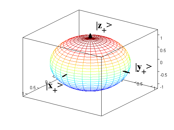
A very useful visualization technique that is limited to two dimensional systems is given by the so called Bloch sphere. By ignoring a physically irrelevant overall phase factor, the general state of a qubit can be written as

(4.1) |ψ=cosθ2|0+eiφsinθ2|1withφ[0,2π),θ[0,π].formulae-sequenceket𝜓𝜃2ket0superscript𝑒𝑖𝜑𝜃2ket1withformulae-sequence𝜑02𝜋𝜃0𝜋\left|\psi\right\rangle=\cos\frac{\theta}{2}\left|0\right\rangle+e^{i\varphi}\sin\frac{\theta}{2}\left|1\right\rangle\quad\mbox{\rm with}\quad\varphi\in[0,2\pi),\,\theta\in[0,\pi].

If we interpret θ𝜃\theta and φ𝜑\varphi as spherical coordinates

(4.2) r^=(cosφsinθ,sinφsinθ,cosθ)=(x,y,z),^𝑟𝜑𝜃𝜑𝜃𝜃𝑥𝑦𝑧\hat{r}=(\cos\varphi\sin\theta,\sin\varphi\sin\theta,\cos\theta)=(x,y,z),

every qubit state has a unique representation as a point on the three-dimensional unit sphere, also known as Bloch sphere (see Fig. 5).

The unit-vector r^=r^ψ^𝑟subscript^𝑟𝜓\hat{r}=\hat{r}_{\psi} is called Bloch vector of |ψket𝜓\left|\psi\right\rangle. Bloch vectors have the property that

(4.3) r^ϕ=r^χϕ|χ=0.iffsubscript^𝑟italic-ϕsubscript^𝑟𝜒inner-productitalic-ϕ𝜒0\hat{r}_{\phi}=-\hat{r}_{\chi}\iff\left\langle\phi|\chi\right\rangle=0.

For density operators of a two-dimensional system a similar generalization exists. By again ignoring an overall phase, any single qubit density operator can be written as (see [18])

(4.4) ρ=12(1+zxiyx+iy1z).𝜌121𝑧𝑥𝑖𝑦𝑥𝑖𝑦1𝑧\rho=\frac{1}{2}\left(\begin{array}[]{cc}1+z&x-iy\\ x+iy&1-z\end{array}\right).

For mixed states, the Bloch vector rρ=(x,y,z)subscript𝑟𝜌𝑥𝑦𝑧r_{\rho}=(x,y,z) lies inside the Bloch sphere (rρ<1normsubscript𝑟𝜌1\|r_{\rho}\|<1) and for a classical unbiased coin flip state, i.e. p(|0)=p(|1)=1/2𝑝ket0𝑝ket112p(\left|0\right\rangle)=p(\left|1\right\rangle)=1/2 we get

(4.5) ρc=(120012)rρc=(0,0,0).\rho_{c}=\left(\begin{array}[]{cc}\frac{1}{2}&0\\ 0&\frac{1}{2}\end{array}\right)\quad\Rightarrow r_{\rho_{c}}=(0,0,0).

Unfortunately, there is no easy generalization of the Bloch sphere for higher dimensional quantum systems.

5. A New Approach to Signal Segmentation using Conjugate Information Variables

The segmentation of signals is one of the fundamental problems in the area of signal and image processing. This is especially true as many higher-level signal analysis algorithms rely heavily on the result of a low-level segmentation process. The term segmentation is mostly not well defined as it can refer to finding some objects in an image, e.g. a face, skin, coin, etc., or detecting lower-level features like edges, constant signal areas, etc.

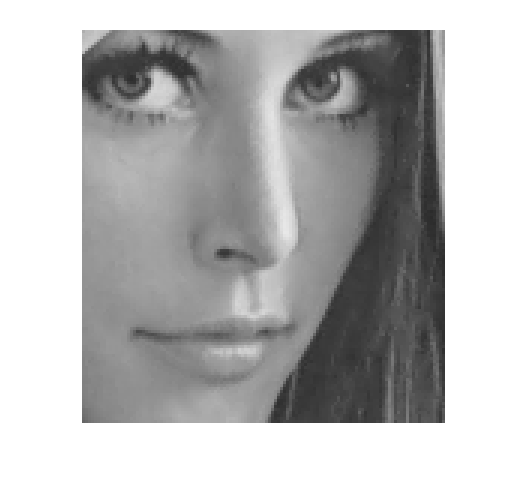
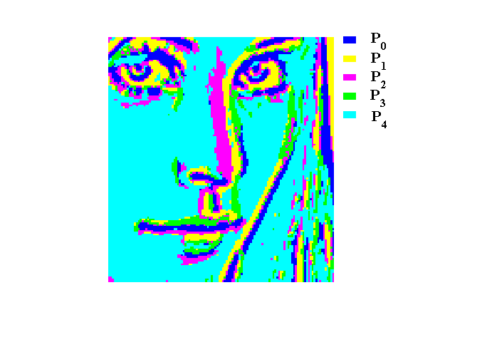
In this chapter we suggest a new approach for a specific segmentation problem, namely the segmentation of signals into locally constant, rising or falling parts, and minima or maxima. For simplicity we assume one-dimensional signals but remark that the approach is not limited to this and can be extended to two- or higher-dimensional problems (see Fig. 6).

Let the signal be given by f(t)𝑓𝑡f(t) and let it be at least twice differentiable, that is f(t)superscript𝑓𝑡f^{{}^{\prime}}(t) and f′′(t)superscript𝑓′′𝑡f^{{}^{\prime\prime}}(t) exist. In our approach the deriviates will be used as as conjugate variables in order to classify local parts of functions.

We need the range of the derivatives to be within certain limits to normalize them properly. This can sometimes cause problems as we have to think about meaningful limits in a given application but usually the limits are obvious for real life signals, such as an image function where the pixel’s range from zero to one, etc. The limits of the derivatives will be used as soft thresholds that control each other.

Zero crossings of the first derivative indicate extrema of a function and the sign of the second dervative destincts between a maximum and a minimum. The function is constant or has a saddle point if both derivatives are zero. In the presence of noise zero crossings of the first derivative becomes unstable whereas the sign of the second derivative remains robust unless there is a saddle point. We will expoit this fact and relate it the role amplitude and phase play for qubits.

Let

p±(t)superscript𝑝plus-or-minus𝑡\displaystyle p^{\pm}(t) =\displaystyle= c2±f′′(t)2c2,plus-or-minussubscript𝑐2superscript𝑓′′𝑡2subscript𝑐2\displaystyle\sqrt{\frac{c_{2}\pm f^{{}^{\prime\prime}}(t)}{2c_{2}}},
α+(t)superscript𝛼𝑡\displaystyle\alpha^{+}(t) =\displaystyle= p+(t)eiπf(t)/c1,superscript𝑝𝑡superscript𝑒𝑖𝜋superscript𝑓𝑡subscript𝑐1\displaystyle p^{+}(t)e^{i\pi f^{{}^{\prime}}(t)/c_{1}},
α(t)superscript𝛼𝑡\displaystyle\alpha^{-}(t) =\displaystyle= p(t),superscript𝑝𝑡\displaystyle p^{-}(t),
with |f(t)|c1,|f′′(t)|c2formulae-sequencesuperscript𝑓𝑡subscript𝑐1superscript𝑓′′𝑡subscript𝑐2|f^{{}^{\prime}}(t)|\leq c_{1},|f^{{}^{\prime\prime}}(t)|\leq c_{2} for all t𝑡t,

and define quantum states

(5.1) |ψ(t)=α+(t)|z++α(t)|z.ket𝜓𝑡superscript𝛼𝑡ketsubscript𝑧superscript𝛼𝑡ketsubscript𝑧\left|\psi(t)\right\rangle=\alpha^{+}(t)\left|z_{+}\right\rangle+\alpha^{-}(t)\left|z_{-}\right\rangle.

Please note that as |α+(t)|2+|α(t)|2=1superscriptsuperscript𝛼𝑡2superscriptsuperscript𝛼𝑡21|\alpha^{+}(t)|^{2}+|\alpha^{-}(t)|^{2}=1, for all t𝑡t, the |ψ(t)ket𝜓𝑡\left|\psi(t)\right\rangle are well-defined qubits. |z+,|zketsubscript𝑧ketsubscript𝑧\left|z_{+}\right\rangle,\left|z_{-}\right\rangle describe the positive and negative z𝑧z-axis of the Bloch sphere (see Fig. 5) and f′′(t)=±c2|ψ(t)=|z±superscript𝑓′′𝑡plus-or-minussubscript𝑐2ket𝜓𝑡ketsubscript𝑧plus-or-minusf^{{}^{\prime\prime}}(t)=\pm c_{2}\Longleftrightarrow\left|\psi(t)\right\rangle=\left|z_{\pm}\right\rangle independent of f(t)superscript𝑓𝑡f^{{}^{\prime}}(t). The positive and negative x𝑥x and y𝑦y axis respectively are given by

|x+ketsubscript𝑥\displaystyle\left|x_{+}\right\rangle =12(|z++|z),absent12ketsubscript𝑧ketsubscript𝑧\displaystyle=\frac{1}{\sqrt{2}}(\left|z_{+}\right\rangle+\left|z_{-}\right\rangle),\quad |x=12(|z+|z),ketsubscript𝑥12ketsubscript𝑧ketsubscript𝑧\displaystyle\left|x_{-}\right\rangle=\frac{1}{\sqrt{2}}(\left|z_{+}\right\rangle-\left|z_{-}\right\rangle),
|y+ketsubscript𝑦\displaystyle\left|y_{+}\right\rangle =12(|z++i|z),absent12ketsubscript𝑧𝑖ketsubscript𝑧\displaystyle=\frac{1}{\sqrt{2}}(\left|z_{+}\right\rangle+i\left|z_{-}\right\rangle),\quad |y=12(|z+i|z).ketsubscript𝑦12ketsubscript𝑧𝑖ketsubscript𝑧\displaystyle\left|y_{-}\right\rangle=\frac{1}{\sqrt{2}}(\left|z_{+}\right\rangle-i\left|z_{-}\right\rangle).

f′′(t)=f(t)=0|ψ(t)=|x+superscript𝑓′′𝑡superscript𝑓𝑡0ket𝜓𝑡ketsubscript𝑥f^{{}^{\prime\prime}}(t)=f^{{}^{\prime}}(t)=0\Longleftrightarrow\left|\psi(t)\right\rangle=\left|x_{+}\right\rangle whereas f′′(t)=0f(t)=±c1|ψ(t)=|xsuperscript𝑓′′𝑡0superscript𝑓𝑡plus-or-minussubscript𝑐1ket𝜓𝑡ketsubscript𝑥f^{{}^{\prime\prime}}(t)=0\wedge f^{{}^{\prime}}(t)=\pm c_{1}\Longleftrightarrow\left|\psi(t)\right\rangle=\left|x_{-}\right\rangle. f(t)superscript𝑓𝑡f^{{}^{\prime}}(t) and f′′(t)superscript𝑓′′𝑡f^{{}^{\prime\prime}}(t) are now conjugate variables in the sense that observing the random variables X={|x+x+|,|xx|}𝑋ketsubscript𝑥brasubscript𝑥ketsubscript𝑥brasubscript𝑥X=\{\left|x_{+}\right\rangle\left\langle x_{+}\right|,\left|x_{-}\right\rangle\left\langle x_{-}\right|\} and Z={|z+z+|,|zz|}𝑍ketsubscript𝑧brasubscript𝑧ketsubscript𝑧brasubscript𝑧Z=\{\left|z_{+}\right\rangle\left\langle z_{+}\right|,\left|z_{-}\right\rangle\left\langle z_{-}\right|\} the commutator333The commutator of two operators A,B𝐴𝐵A,B is given by [A,B]=ABBA𝐴𝐵𝐴𝐵𝐵𝐴[A,B]=AB-BA. Two operators commute if and only if their commutator equals zero, i.e. AB=BA[A,B]=0.𝐴𝐵𝐵𝐴𝐴𝐵0AB=BA\Longleftrightarrow[A,B]=0. between any two projectors of X𝑋X and Z𝑍Z becomes maximal:

A±=|x±x±|,B±=|z±z±|A±B±B±A±=12.formulae-sequencesubscript𝐴plus-or-minusketsubscript𝑥plus-or-minusbrasubscript𝑥plus-or-minussubscript𝐵plus-or-minusketsubscript𝑧plus-or-minusbrasubscript𝑧plus-or-minusnormsubscript𝐴plus-or-minussubscript𝐵plus-or-minussubscript𝐵plus-or-minussubscript𝐴plus-or-minus12A_{\pm}=\left|x_{\pm}\right\rangle\left\langle x_{\pm}\right|,B_{\pm}=\left|z_{\pm}\right\rangle\left\langle z_{\pm}\right|\Rightarrow\|A_{\pm}B_{\pm}-B_{\pm}A_{\pm}\|=\frac{1}{2}.
Refer to caption
Refer to caption
Refer to caption
Refer to caption
Refer to caption
Refer to caption
Refer to caption
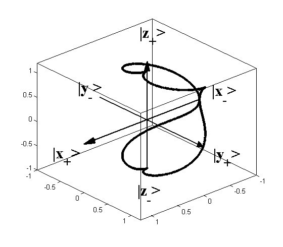
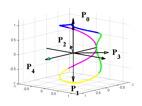
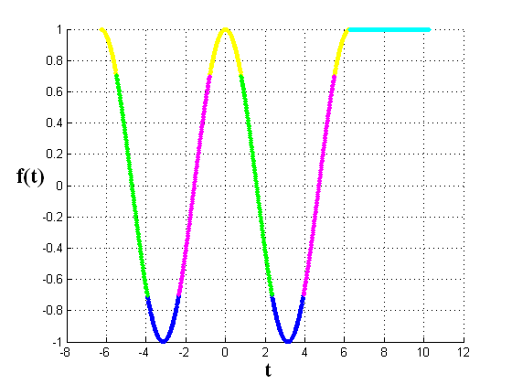
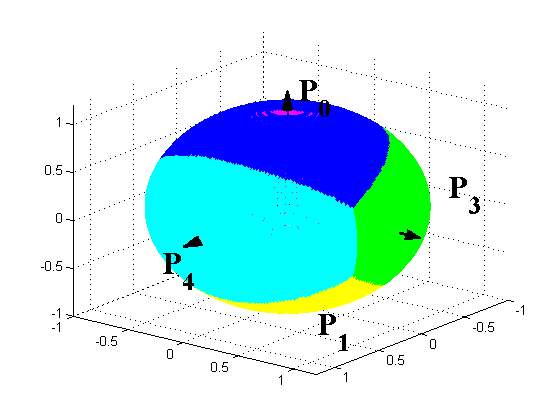
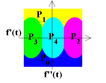
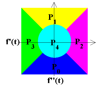
Figure 5. Top left: Bloch sphere representation of all qubit states. Top right: Bloch sphere representation of the qubit states |ψ(t)ket𝜓𝑡\left|\psi(t)\right\rangle for f(t)𝑓𝑡f(t) as given in Equation 5.2. Middle left: Labeling result in the Bloch sphere representation. Middle right: Labeling of f(t)𝑓𝑡f(t). Bottom left: Decision regions in the Bloch sphere representation, P2subscript𝑃2P_{2} is shining through at the north pole but is not visible from this perspective. Bottom middle: Decision regions over the joint distribution of f′′(t)superscript𝑓′′𝑡f^{{}^{\prime\prime}}(t) and f(t)superscript𝑓𝑡f^{{}^{\prime}}(t). Bottom right: Model based (see Equations 5.3) decision regions over the joint distribution of f′′(t)superscript𝑓′′𝑡f^{{}^{\prime\prime}}(t) and f(t)superscript𝑓𝑡f^{{}^{\prime}}(t). The limits of the axes are ±c1plus-or-minussubscript𝑐1\pm c_{1} for f(t)superscript𝑓𝑡f^{{}^{\prime}}(t) and ±c2plus-or-minussubscript𝑐2\pm c_{2} for f′′(t)superscript𝑓′′𝑡f^{{}^{\prime\prime}}(t). If c=c1=c2𝑐subscript𝑐1subscript𝑐2c=c_{1}=c_{2}, the radius of the inner circle, P4subscript𝑃4P_{4}, is given by c/2𝑐2c/2.

Next we define a set of projectors:

P0subscript𝑃0\displaystyle P_{0} =\displaystyle= |z+z+|ketsubscript𝑧brasubscript𝑧\displaystyle\left|z_{+}\right\rangle\left\langle z_{+}\right|
P1subscript𝑃1\displaystyle P_{1} =\displaystyle= |zz|ketsubscript𝑧brasubscript𝑧\displaystyle\left|z_{-}\right\rangle\left\langle z_{-}\right|
P2subscript𝑃2\displaystyle P_{2} =\displaystyle= 12(|yy|+|xx|)=12(P012(1+i)P1)12ketsubscript𝑦brasubscript𝑦ketsubscript𝑥brasubscript𝑥12subscript𝑃0121𝑖subscript𝑃1\displaystyle\frac{1}{\sqrt{2}}\left(\left|y_{-}\right\rangle\left\langle y_{-}\right|+\left|x_{-}\right\rangle\left\langle x_{-}\right|\right)=\frac{1}{\sqrt{2}}\left(P_{0}-\frac{1}{\sqrt{2}}(1+i)P_{1}\right)
P3subscript𝑃3\displaystyle P_{3} =\displaystyle= 12(|y+y+|+|xx|)=12(P012(1i)P1)12ketsubscript𝑦brasubscript𝑦ketsubscript𝑥brasubscript𝑥12subscript𝑃0121𝑖subscript𝑃1\displaystyle\frac{1}{\sqrt{2}}\left(\left|y_{+}\right\rangle\left\langle y_{+}\right|+\left|x_{-}\right\rangle\left\langle x_{-}\right|\right)=\frac{1}{\sqrt{2}}\left(P_{0}-\frac{1}{\sqrt{2}}(1-i)P_{1}\right)
P4subscript𝑃4\displaystyle P_{4} =\displaystyle= |x+x+|=12(P0+P1)=12𝕀.ketsubscript𝑥brasubscript𝑥12subscript𝑃0subscript𝑃112𝕀\displaystyle\left|x_{+}\right\rangle\left\langle x_{+}\right|=\frac{1}{\sqrt{2}}\left(P_{0}+P_{1}\right)=\frac{1}{\sqrt{2}}\mathbb{I}.

Only P0subscript𝑃0P_{0} and P1subscript𝑃1P_{1} form a random variable as they add up to the identity and therefore fulfill the completeness condition. They indicate minimum or maximum of the function. Pi,i=2,,4formulae-sequencesubscript𝑃𝑖𝑖24P_{i},i=2,\ldots,4 would have to be complemented by 𝕀Pi𝕀subscript𝑃𝑖\mathbb{I}-P_{i} in order to do so. The choice of projectors depends on the problem we want to solve.

For any given f(t)𝑓𝑡f(t) we now can project the corresponding |ψ(t)ket𝜓𝑡\left|\psi(t)\right\rangle and get a classification result by maximizing over all projectors

C(f(t))=i{0,,4}:ψ(t)|Pi|ψ(t)=maxj=0,,4ψ(t)|Pjψ(t).:𝐶𝑓𝑡𝑖04quantum-operator-product𝜓𝑡subscript𝑃𝑖𝜓𝑡subscript𝑗04conditional𝜓𝑡subscript𝑃𝑗𝜓𝑡C(f(t))=i\in\{0,\ldots,4\}:\left\langle\psi(t)\right|P_{i}\left|\psi(t)\right\rangle=\max_{j=0,\ldots,4}\left\langle\psi(t)\right|P_{j}\left|\psi(t)\right\rangle.

Alternatively, if Xi={Pi,𝕀Pi}={|χi,0χi,0|,|χi,1χi,1|},i=0,,4formulae-sequencesubscript𝑋𝑖subscript𝑃𝑖𝕀subscript𝑃𝑖ketsubscript𝜒𝑖0brasubscript𝜒𝑖0ketsubscript𝜒𝑖1brasubscript𝜒𝑖1𝑖04X_{i}=\{P_{i},\mathbb{I}-P_{i}\}=\{\left|\chi_{i,0}\right\rangle\left\langle\chi_{i,0}\right|,\left|\chi_{i,1}\right\rangle\left\langle\chi_{i,1}\right|\},i=0,\ldots,4, and |χket𝜒\left|\chi\right\rangle represents the eigenvector of the corresponding projector, we can minimize the distance D(|χi,0,|ψ(t))𝐷ketsubscript𝜒𝑖0ket𝜓𝑡D(\left|\chi_{i,0}\right\rangle,\left|\psi(t)\right\rangle).

Refer to caption
Refer to caption
Refer to caption
Refer to caption
Figure 6. An application of the segmentation technique. The original image on the top left was smoothed on the constant part P4subscript𝑃4P_{4} of the image function as given in the bottom right picture. The result of smoothing adaptively with an average filter (15×15151515\times 15) is shown in the lower left picture (P0,,P3subscript𝑃0subscript𝑃3P_{0},\dots,P_{3} are not filtered). The top right shows the filter result using the same filter kernel independent of the image content.

The results of the classification for an analytic function

(5.2) f(t)={cos(t),|t|<2π1,t>2π𝑓𝑡cases𝑡𝑡2𝜋1𝑡2𝜋f(t)=\left\{\begin{array}[]{cc}\cos(t),&|t|<2\pi\\ 1,&t>2\pi\end{array}\right.

are given in middle row of Fig. 5, whereas the bottom row (left and middle picture) shows the decision boundaries over the entire joint distribution of the derivatives as derived by the described approach. Usually we cannot access an analytic expression for f(t)𝑓𝑡f(t) but a measurement of either f(t)𝑓𝑡f(t) or f(t)superscript𝑓𝑡f^{{}^{\prime}}(t) and f′′(t)superscript𝑓′′𝑡f^{{}^{\prime\prime}}(t) is available. If we measure f(t)𝑓𝑡f(t) we have to derive the derivatives numerically444Depending on the application, this might require some low pass filtering of the measurements to gain stability in the derivatives.. An example for the measurement of f(t)superscript𝑓𝑡f^{{}^{\prime}}(t) and f′′(t)superscript𝑓′′𝑡f^{{}^{\prime\prime}}(t) is given by observing the velocity and acceleration of an object. In general these measurement will be taken by independent devices but they are highly correlated quantities.

In either case the measurements will be subject to errors. We may choose different error models for the respective areas. In the example we gave in the introduction we could decide that the acoustic signal is mainly noise during the day time and the visual signal is not available at night time. Towards the poles of the Bloch sphere the phase term (in this case f(t)superscript𝑓𝑡f^{{}^{\prime}}(t)) becomes less important as it seamlessly transforms itself into a global phase factor. In equatorial regions it becomes predominant. A quantitative discussion of this depends on the concrete problem to be solved, especially on the statistical error model(s) to be chosen, and shall be left for a future publication.

A standard approach to derive the decision regions would be to create a model of the decision problem and than minimize some distance function over the entire joint signal distribution to this model as shown in the bottom right picture of Fig. 5 for the function given in Equation 5.2. To derive this model we have to notice the (partially) nonlinear dependency of

f(t)=sin(t),f′′(t)=cos(t),f(t)2+f′′(t)2=1,formulae-sequencesuperscript𝑓𝑡𝑡formulae-sequencesuperscript𝑓′′𝑡𝑡superscript𝑓superscript𝑡2superscript𝑓′′superscript𝑡21\displaystyle f^{{}^{\prime}}(t)=-\sin(t),\quad f^{{}^{\prime\prime}}(t)=-\cos(t),\quad f^{{}^{\prime}}(t)^{2}+f^{{}^{\prime\prime}}(t)^{2}=1, |t|<2π,𝑡2𝜋\displaystyle|t|<2\pi,
(5.3) f(t)=f′′(t)=0,superscript𝑓𝑡superscript𝑓′′𝑡0\displaystyle f^{{}^{\prime}}(t)=f^{{}^{\prime\prime}}(t)=0, t2π.𝑡2𝜋\displaystyle t\geq 2\pi.

In this model the decision depends on both signals over (almost) the entire joint distribution range, whereas the model derived from the conjugate variables cuts off the influence of one signal around the poles of the Bloch sphere.

6. Discussion

The approach of modelling joint distributions of signals as conjugate variables certainly has its limitations. We remark that its strengthes go along with its weaknesses. Whenever all signals are meaningful over the entire joint distribution range other approaches might be more successful555In the Hilbert space setting used in this paper we need a higher dimensional system, e.g. a two qubit system. Of course, we may add conjugate information to each of those systems, if it is available to us..

On the other hand in situations where we have an expectation that we can rely on some signals more than others, depending on some given (or derived) parameters, our approach will be valuable as this dependency may be modelled directly. It is noteworthy that the role of the two signals used for the encoding might be quite different. In the bird example we may classify the two species, lets call them Happy and Unhappy, using the acoustic signal alone at times but even when this signal becomes mixed we still can rely on its presence and then take the optical signal into account. The converse is not true as we can not speak about a colour at night. Therefore, the optical sensor (used as phase information) might give arbitrary measurement results (including blue or green!) at night time. This will not influence the classification result as the measurement of the conjugate acoustic signal is mapped to one of the polar regions at night time. In lucky circumstances, e.g. when by chance we have no background noise during the day or the moon provides enough light at night, the joint observation of chirp and colour does not change the classification result either, as a Happy bird does not become more Happy if we know both features. When the noise level is slowly increasing (at sunrise or sunset) seamlessly both signals contribute to the classification and allow a discrimination of the two classes.

Just to give a flavour of the results to expect, Fig. 6 shows the application of an adaptive filter on image functions that is based on the segmentation approach. At the top left the original image (used as the signal f(t)𝑓𝑡f(t)) is given which is to be smoothed to remove noise introduced by the sensor (camera, scanner, etc.). If we assume uniform noise, we can remove this by averaging over small parts of the image function. The application of an average filter independent of the image structure will remove this noise but unfortunately it will remove parts of the image content at the same time as can be seen in the top right picture of Fig. 6. If we classify each point of the image according to the approach described in Section 5, we can apply the averaging process only to image areas that are labelled constant, i.e. P4subscript𝑃4P_{4} (Fig. 6 bottom right). This results in an image that is fairly smooth in these constant image areas but untouched everywhere else (Fig. 6 bottom left). In the other areas we could apply different filter kernels (and different error models) if we wish to do so.

7. Conclusion and Future Work

In this paper we have described a method for modelling joint distributions of signals as conjugate variables in finite-dimensional complex Hilbert spaces. We have derived a distance function based on the transition probability of quantum states that is a metric on pure states and satisfies the triangle inequality for mixed states, and we have related it to some distance functions between probability distributions. The analysis of other distance measures on quantum states, especially the so called trace distance which is closely related to the variational distance of probability distributions, will be a future task.

We believe that the mathematical concept of quantum information theory offers a fertile resource in many areas of information processing. In this article we mainly focused on non-decomposed principle systems, but it would be very interesting to analyze the decomposition of higher-dimensional systems which remains a future task. We have not touched on the field of quantum operations, i.e unitary transformations of quantum states which again offers a rich potential. Additionally generalized measurement operators (positive operator valued measurements (POVM)) offer a valuable future research direction. The use of Wigner functions provides another promising research area. Wigner functions relate the probability distributions of conjugate variables to each other as they describe this joint (real valued) distribution. Moreover they relate the spatial to the frequency domain, which may have further impact.

References

  • [1] F. J. Aherne, N. A. Thacker, and P.I. Rockett, The Bhattacharyya metric as an absolute similarity measure for frequency coded data, Kypernetika 32 (1997), no. 4, 001–007.
  • [2] Robert B. Ash, Information theory, Dover Publication, Inc., New York, 1965.
  • [3] O. E. Barndorff-Nielsen, R. D. Gill, and P. E. Jupp, On quantum statistical inference, J. Roy. Statist. Soc. (B) 65 (2003), 775–816.
  • [4] D.C. Brody and L.P. Hughston, Quantum noise and stochastic reduction, Journal of Physics A, MATH GEN 39 (2006), 833–876, ISSN: 0305-4470.
  • [5] M. W. Coffey, Properties and possibilities of quantum shapelets, Journal of Physics A 39 (2006), 877–887.
  • [6] D. Comaniciu, V. Ramesh, and P. Meer, Kernel-based object tracking, IEEE Transactions on Pattern Analysis and Machine Intelligence 25 (2003), no. 5, 564–577.
  • [7] T.M. Cover and J.A. Thomas, Elements of information theory, 1st ed., John Wiley &\& Sons, New York, 1991.
  • [8] Yonina C. Eldar and Alan V. Oppenheim, Quantum signal processing, IEEE Signal Processing Magazine (2002).
  • [9] C. A. Fuchs, Distinguishability and accessible information in quantum theory, Online preprint quant-ph/9601020, 1996.
  • [10] Robert G. Gallager, Information theory and reliable communication, John Wiley &\& Sons, New York, 1968.
  • [11] Lov Grover and Terry Rudolph, Creating superpositions that correspond to efficiently integrable probability distributions, http://arxiv.org/abs/quant-ph/0208112, 2002.
  • [12] Josef Gruska, Quantum computing, McGraw-Hill, London, 1999.
  • [13] C. W. Helstrom, Quantum detection and estimation theory, Academic Press, New York, 1976.
  • [14] Ulrike Herzog and János A. Bergou, Distinguishing mixed quantum states: Minimum-error discrimination versus optimum unambiguous discrimination, Phys. Rev. A 70 (2004), no. 2, 022302.
  • [15] A.S. Holevo, Probabilistic and statistical aspect of quantum theory, North Holland, P.C., 1982.
  • [16] Solomon Kullback, Information theory and statistics, Dover Publication, Inc., New York, 1997.
  • [17] J. Lin, Divergence measures based on the Shannon entropy, IEEE Transactions on Information Theory 37 (1991), no. 1, 145–151.
  • [18] Zdzislaw Meglicki, Introduction to quantum computing (m743), http://beige.ucs.indiana.edu/M743/, April 2005.
  • [19] Michael A. Nielsen and Isaac L. Chuang, Quantum computation and quantum information, Cambridge University Press, 2000.
  • [20] Michael Nölle and Bernhard Ömer, Representation of cyclic colour spaces within quantum space, Proceedings of the 8thsuperscript8𝑡8^{th} International Conference on Digital Image Computing - Techniques and Applications (DICTA’05) (2005).
  • [21] Michael Nölle, Bernhard Ömer, and Martin Suda, Quantum information algorithms - new solutions for known problems, e &\& i Elektrotechnik und Informationstechnik, Springer Wien 124 (2007), no. 5.
  • [22] Puzicha, J., Rubner, Y., Tomasi, C., and Buhmann, J. M., Empirical Evaluation of Dissimilarity Measures for Color and Texture, Proc. of the International Conference on Computer Vision (ICCV’99), 1999, pp. 1165–1173.
  • [23] M. Zaharieva, R. Huber-Mörk, M. Nölle, and M. Kampel, On ancient coin classification, International Symposium on Virtual Reality, Archaeology and Cultural Heritage VAST, 20078thsuperscript8𝑡8^{th} (2007).