Density of States of Quantum Spin Systems from Isotropic Entanglement

Abstract

We propose a method which we call “Isotropic Entanglement” (IE), that predicts the eigenvalue distribution of quantum many body (spin) systems (QMBS) with generic interactions. We interpolate between two known approximations by matching fourth moments. Though, such problems can be QMA-complete, our examples show that IE provides an accurate picture of the spectra well beyond what one expects from the first four moments alone. We further show that the interpolation is universal, i.e., independent of the choice of local terms.

I A highly accurate match (better than four moments).

We propose a method to compute the “density of states” (DOS) or “eigenvalue density” of quantum spin systems with generic local interactions IE . More generally one wishes to compute the DOS of the sum of non-commuting random matrices from their, individually known, DOS’s.

We begin with an example in Figure 1, where we compare exact diagonalization against two approximations that we considered early in our work and our method IE .

• Dashed grey curve: classical approximation. Notice that it overshoots to the right.

• Solid grey curve: isotropic approximation (or iso). Notice that it overshoots to the left.

• Solid black curve: isotropic entanglement (IE).

• Dots: exact diagonalization of the quantum problem given in Eq. 1.

Figure 1: The exact diagonalization in dots and IE compared to the two approximations. The title parameters are explained in the section on numerical results.

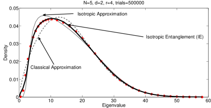
The classical approximation ignores eigenvector structure by summing random eigenvalues uniformly from non-commuting matrices. The curve is the convolution of the probability densities of the eigenvalues of each matrix.

The isotropic approximation assumes that the eigenvectors are in “general position”; that is, we add the two matrices with correct eigenvalue densities but choose the eigenvectors from Haar (uniform) measure. As the matrix size goes to infinity, the resulting distribution has been popularized recently as the free convolution of the individual distributions IE , or (speicher, , for a nice exposition).

The exact diagonalization given by red dots, the dashed and solid grey curves have exactly the same first three moments, but differing fourth moments.

Isotropic Entanglement (IE) is a linear combination of the two approximations obtained by matching the fourth moments. We show 1) the fit is better than what might be expected by the first four moments alone, 2) the combination is always convex for the problems of interest, given by a $0\leq p\leq 1$, and 3) this convex combination is universal depending on the parameter counts of the problem but not the eigenvalue densities of the local terms.

Parameter counts: exponential, polynomial and zero.—Because of the locality of generic interactions, the complete set of eigenstates has parameter count equal to a polynomial in the number of spins, though the dimensionality is exponential. The classical and isotropic approximations have zero and exponentially many random parameters respectively. This suggests that the problem of interest somehow lies between the two approximations.

II Physical implications and problem formulation.

QMBS spectra have been elusive for two reasons: 1. The terms that represent the interactions are generally non-commuting. This is particularly pronounced for systems with random interactions (e.g., quantum spin glasses (sachdev, , p. 320)spinGlass ; sachdev2 ). 2. Standard numerical diagonalization is limited by memory and computer speed because of exponential growth. Energy eigenvalue distributions are needed for calculating the partition function $Z$. Exact calculation of the spectrum of interacting QMBS has been shown to be difficult schuch .

Though, much progress has been made in understanding the ground states of interacting QMBS cirac ; vidal ; white ; wen ; frank ; hastings ; ramis , eigenvalue distributions are less studied. An accurate description of tails of distributions are desirable for condensed matter physics. IE provides a direct method for obtaining eigenvalue distributions of quantum spin systems with generic local interactions (i.e., quantum spin systems) and does remarkably well at approximating the tails.

Though we are not restricted to one dimensional chains, for sake of concreteness, we investigate $N$ interacting $d$-dimensional quantum spins (qudits) on a line with generic interactions. The Hamiltonian is

$$H=\sum_{l=1}^{N-1}\mathbb{I}_{d^{l-1}}\otimes H_{l,\cdots,l+L-1}\otimes\mathbb{I}_{d^{N-l-\left(L-1\right)}},$$ (1)

where the local terms $H_{l,\cdots,l+L-1}$ are finite $d^{L}\times d^{L}$ random matrices. From now on we take the case of nearest neighbors interactions, $L=2$, unless otherwise specified.

The eigenvalue distribution of any commuting subset of $H$ such as the terms with $l$ odd (the “odds”) or $l$ even (the “evens”) can be obtained using local diagonalization. However, the difficulty in approximating the full spectrum of $H\equiv H_{\mbox{odd}\vphantom{\mbox{even}}}+H_{\mbox{even}\vphantom{\mbox{odd}}}$ is in summing the odds and the evens because of their overlap at every site.

The intuition behind IE is that terms with an overlap, such as $H_{l,l+1}$ and $H_{l+1,l+2}$, introduce randomness and mixing through sharing of a site. Namely, the process of entanglement generation introduces an isotropicity between the eigenvectors of evens and odds that can be harnessed to capture the spectrum.

III Isotropic entanglement.

Let $A$ and $B$ denote diagonal matrices containing the eigenvalues, in random order, of the odds and evens respectively. In a basis where (at least) the odds are diagonal, our approximations to the Hamiltonian in Eq. 1 become

Classical: $$H^{c}=A+B$$

Isotropic: $$H^{iso}=A+Q^{-1}BQ,$$ (2)

where $Q$ is a $\beta-$Haar measure orthogonal matrix of size $d^{N}$ with $\beta=1$ corresponding to real orthogonals, $\beta=2$ unitaries, and $\beta=4$ quaternions (see alanGhost for formal treatment of a general $\beta$).

The Hamiltonian given by Eq. 1 in a basis where the odds are diagonal is

$$\mbox{Quantum: }H=A+Q_{q}^{-1}BQ_{q}.$$ (3)

The $Q_{q}$ has the formidable form $Q_{q}=\left(Q_{A}\right)^{-1}Q_{B}$, where (for odd number of sites $N$)

$$Q_{A}= Q_{1}\otimes Q_{3}\otimes\cdots\otimes Q_{N-2}\otimes\mathbb{I}_{d}$$

$$Q_{B}= \mathbb{I}_{d}\otimes Q_{2}\otimes Q_{4}\otimes\cdots\otimes Q_{N-1}.$$ (4)

The eigenvalue distribution of Eq. 3 is what we are after.

To establish the plausibility of the classical and isotropic approximations, we consider the moments. In general we have the $k^{\textrm{th}}$ moments

$$m_{k}^{c}= \frac{1}{d^{N}}\mathbb{E}\textrm{Tr}\left(A+B\right)^{k},$$

$$m_{k}^{iso}= \frac{1}{d^{N}}\mathbb{E}\textrm{Tr}\left(A+Q^{-1}BQ\right)^{k}\;\mbox{ and}$$ (5)

$$m_{k}^{q}= \frac{1}{d^{N}}\mathbb{E}\textrm{Tr}\left(A+Q_{q}^{-1}BQ_{q}\right)^{k}.$$

The first three moments are usually encoded as the mean, variance, and skewness; the fourth moment is encoded by the kurtosis which we denote $\gamma_{2}$.

(The Matching Three Moments Theorem) The first three moments of the classical and isotropic approximations exactly match those of the quantum problem IE .

Turning to the fourth moment, we propose to match the kurtosis $\gamma_{2}^{q}$ with a linear combination of the classical ($\gamma_{2}^{c}$) and isotropic ($\gamma_{2}^{iso}$) kurtoses:

$$\gamma_{2}^{q}=p\gamma_{2}^{c}+\left(1-p\right)\gamma_{2}^{iso}\Rightarrow\qquad p=\frac{\gamma_{2}^{q}-\gamma_{2}^{iso}}{\gamma_{2}^{c}-\gamma_{2}^{iso}}.$$ (6)

In terms of probability measures, IE provides

$$d\nu^{q}\approx d\nu^{IE}=pd\nu^{c}+(1-p)d\nu^{iso},$$ (7)

where $d\nu$ denotes a probability measure. So long as $0\leq p\leq 1$, $d\nu^{IE}$ is a probability measure whose first four moments match the theoretical measure $d\nu^{q}$.

In the expansion of the fourth moments, by a theorem we call The Departure TheoremIE , the numerator and the denominator in Eq. 6 respectively become,

$$\gamma_{2}^{q}-\gamma_{2}^{iso}= \frac{2}{d^{N}}\frac{\mathbb{E}\left\{\textrm{Tr}\left[\left(AQ_{q}^{-1}BQ_{q}\right)^{2}-\left(AQ^{-1}BQ\right)^{2}\right]\right\}}{\sigma^{4}}$$

$$\gamma_{2}^{c}-\gamma_{2}^{iso}= \frac{2}{d^{N}}\frac{\mathbb{E}\left\{\textrm{Tr}\left[\left(AB\right)^{2}-\left(AQ^{-1}BQ\right)^{2}\right]\right\}}{\sigma^{4}}.$$ (8)

Evaluation of $p$ in Eq. 6 reduces to the evaluation of the right hand sides of Eq. 8. It is natural to ask, does a $0\leq p\leq 1$ always exist such that the convex combination Eq. 6 can be formed? How would quantum spectra look in the thermodynamical limit ($N\rightarrow\infty$)? The Slider Theorem provides the answers.

(The Slider Theorem) The quantum kurtosis lies in between the classical and the isotropic kurtoses, $\gamma_{2}^{iso}\leq\gamma_{2}^{q}\leq\gamma_{2}^{c}$. Therefore there exists a $0\leq p\leq 1$ such that $\gamma_{2}^{q}=p\gamma_{2}^{c}+\left(1-p\right)\gamma_{2}^{iso}$. Furthermore, $\lim_{N\rightarrow\infty}p=1$.

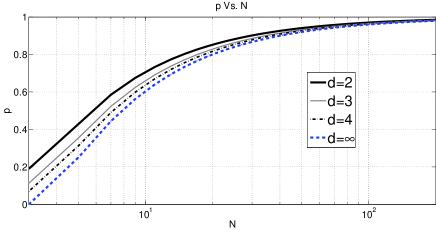
Through our numerical investigations, we observed that $p$ did not change by the choice of local terms; it did not dependent on the covariance matrix. This lead us to prove that $p$ was universal with respect to the choice of generic local terms and allowed us to derive an analytical formula (Figure 2, where we take $\beta=1$).

(Universality Corollary) $p\mapsto p\left(N,d,\beta\right)$, namely, it is independent of the distribution of the local terms (see IE for an analytical formula).

Figure 2: An example where $\beta=1$: the quantum problem for all $d$ lies in between the iso $(p=0)$ and the classical $(p=1)$.

Entanglement shows itself starting at the fourth moment; further, in the expansion of the fourth moments, only the terms that involve a pair of local terms sharing a site differ IE .

Figure 3: $N=11$ with full rank Wishart matrices as local terms.

Figure 4: Approximating the quantum spectrum by $H^{IE}=\sum_{l=1}^{2}Q_{l}^{T}H_{l,\cdots,l+4}Q_{l}$, where the interaction is taken to be $5-$local Wishart matrices.

IV Numerical results.

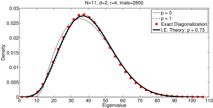
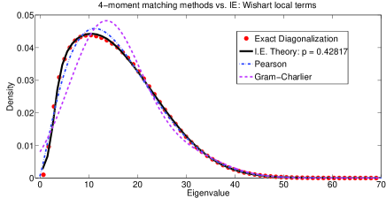
Here we compare our theory against exact diagonalization for various number of sites $N$, local ranks $r$, and site dimensionality $d$. As our first two examples (Figures 1 and 3) we take the local terms to be independent Wishart matrices: Each $H_{l,l+1}=A^{T}A$, where $A$ is a $d^{2}\times d^{2}$ matrix with independent and identically distributed Gaussian random entries. The higher moments of the Wishart matrices were obtained using MOPs mops .

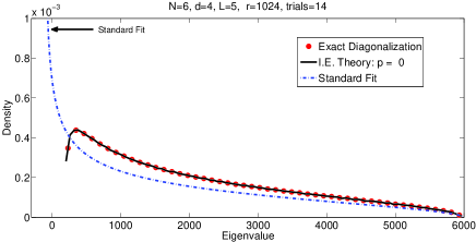
One would expect that $L>2$ would be closer to the isotropic approximation than when the interactions are nearest neighbors because of the larger number of random parameters in Eq. 1. When the number of random parameters of the problem $\left(N-L+1\right)d^{L}$ becomes comparable to $d^{N}$, we indeed find that we can approximate the spectrum with a high accuracy by taking the summands to be all isotropic ramisPI (Figure 4).

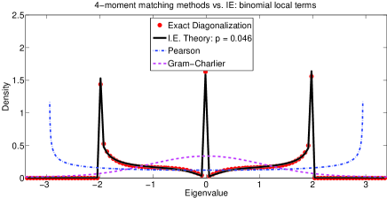
Lastly take the local terms to have Haar eigenvectors but with Bernoulli eigenvalues: $H_{l,l+1}=Q_{l}^{T}\Lambda_{l}Q_{l}$, where $\Lambda_{l}$ is a diagonal matrix of random eigenvalues $\pm 1$ (Figure 5). Here classical treatment leads to a binomial distribution. As expected $p=1$ in Figure 5 has three atoms at $-2,0,2$ corresponding to the randomized sum of the eigenvalues from the two local terms. The exact diagonalization, however, shows that the quantum chain has a much richer structure closer to iso; i.e, $p=0$. This is captured quite well by IE with $p=0.046$.

Figure 5: Local terms have a random binomial distribution.

Figure 6: Summary of Isotropic Entanglement. We have denoted the known classical and isotropic convolutions by $\star$ and $\boxplus_{\mbox{iso}}$ respectively. IE approximates the unknown quantum convolutions $\boxplus_{q}$.

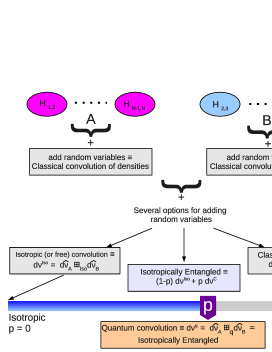
Most distributions built solely from the first four moments would give smooth curves. Roughly speaking, the mean indicates the center of the distribution, variance its width, skewness its bending away from the center and kurtosis how tall and skinny versus how short and fat the distribution is. It is hard to imagine that the kinks, cusps and local extrema of the quantum problem (as seen in some of our examples and in particular Figure 5) could be captured by fitting only the first four moments of the QMBS Hamiltonian to a known distribution. Remarkably a one parameter (i.e., $p$) interpolation between the isotropic and classical suffices in capturing the richness of the spectra of QMBS. Figure 6 summarizes IE.

V Accuracy beyond four moments.

We illustrate in Figures 7 and 8 how the IE fit is better than expected when matching four moments. We used the exact first four moments to approximate the density using the Pearson fit as implemented in MATLAB and also the well-known Gram-Charlier fit Cramer . In Gram it was demonstrated that the statistical mechanics methods for obtaining the DOS, when applied to a finite dimensional vector space, lead to a Gaussian distribution in the lowest order. Further, they showed that successive approximations lead naturally to the Gram-Charlier series Cramer . Comparing these against the accuracy of IE leads us to view IE as more than a moment matching methodology.

Figure 7: IE vs Pearson and Gram-Charlier fits for local terms with binomial distribution

Figure 8: IE vs Pearson and Gram-Charlier fits for local terms with Wishart distribution

VI Outlook.

Our work supports a very general principle that one can obtain an accurate representation of inherently exponential problems dealing with QMBS by approximating them with far less complexity. This realization is at the heart of other recent developments in QMBS research such as Matrix Product States cirac ; vidal , and Density Matrix Renormalization Group white , where the state (usually the ground state of $1D$ chains) can be adequately represented by a Matrix Product State (MPS) ansatz whose parameters grow linearly with the number of quantum particles. Future work includes explicit treatment of fermionic systems and numerical exploration of higher dimensional systems.

We thank Peter W. Shor, Jeffrey Goldstone, Patrick Lee, Peter Young, Gil Strang, Mehran Kardar, Xiao-Gang Wen and Ofer Zeitouni for discussions. We thank the National Science Foundation for support through grants CCF-0829421 and DMS-1035400.

References

- (1) R. Movassagh, A. Edelman, arXiv:1012.5039 (2010)
- (2) A. Nica, R. Speicher, Lectures on the Combinatorics of Free Probability (Cambridge University Press 2006)
- (3) S. Sachdev, Quantum Phase Transitions (Cambridge University Press 2001)
- (4) S. Sachdev Physics World 7, No. 10, 25 (Oct. 1994)
- (5) M. Fannes, B. Nachtergaele, and R. F.Werner, Commun. Math. Phys. 144, 443 (1992)
- (6) B. Brown, S. T. Flammia, N. Schuch, Phys. Rev. Lett. 107, 040501 (2011)
- (7) A. Ambainis, A. W. Harrow, M B. Hastings, arXiv:0910.0472v2 (2010)
- (8) D. Perez-Garcia, F. Verstraete, M. M. Wolf, and J. I. Cirac, Quantum Inf. Comput. 7, 401 (2007)
- (9) G. Vidal, Phys. Rev. Lett. 93, 040502 (2004). See cirac for an alternative proof.
- (10) S. R. White, Phys. Rev. Lett. 69, 2863 (1992)
- (11) Z. C. Gu, M. Levin, and X. G. Wen, Phys. Rev. B 78, 205116 (2008)
- (12) F. Verstraete, V. Murg, and J. I. Cirac, Adv. Phys. 57, 143 (2008)
- (13) R. Movassagh, E. Farhi, J. Goldstone, D. Nagaj, T. J. Osborne, P. W. Shor, Phys. Rev. A 82, 012318 (2010)
- (14) A. Edelman, pp. 783-790. Volume 16 Issue 4 (2010)
- (15) I. Dumitriu, A. Edelman and G. Shuman, Journal of Symbolic Computation 42, 587-620 (2007)
- (16) R. Movassagh, A. Edelman, Talk given at The Perimeter Institute (July 2010): pirsa.org/index.php?p=speaker&name=Ramis_Movassagh
- (17) H. Cramér, Mathematical Methods of Statistics, (Princeton University Press, Princeton 1957)
- (18) S. Das Guptaa, R. K. Bhaduri, Physics Letters B, vol 58 issue 4, 381-383 (1975)