Planar and Spherical Stick Indices of Knots

Abstract.

The stick index of a knot is the least number of line segments required to build the knot in space. We define two analogous 2-dimensional invariants, the planar stick index, which is the least number of line segments in the plane to build a projection, and the spherical stick index, which is the least number of great circle arcs to build a projection on the sphere. We find bounds on these quantities in terms of other knot invariants, and give planar stick and spherical stick constructions for torus knots and for compositions of trefoils. In particular, unlike most knot invariants,we show that the spherical stick index distinguishes between the granny and square knots, and that composing a nontrivial knot with a second nontrivial knot need not increase its spherical stick index.

1. Introduction

The stick index $s[K]$ of a knot type $[K]$ is the smallest number of straight line segments required to create a polygonal conformation of $[K]$ in space. The stick index is generally difficult to compute. However, stick indices of small crossing knots are known, and stick indices for certain infinite categories of knots have been determined:

Theorem 1.1 ([Jin97]).

If $T_{p,q}$ is a $(p,q)$-torus knot with $p<q<2p$, $s[T_{p,q}]=2q$.

Theorem 1.2 ([ABGW97]).

If $nT$ is a composition of $n$ trefoils, $s[nT]=2n+4$.

Despite the interest in stick index, two-dimensional analogues have not been studied in depth. In a recent paper, Adams and Shayler [AS09] defined a new invariant, the projective stick index. We modify their definition slightly:

Definition 1.3.

A planar stick diagram of a knot type $[K]$ is a closed polygonal curve in the plane, with crossing information assigned to self-intersections, that represents $[K]$. The planar stick index $\operatorname{pl}[K]$ of a knot type is the smallest number of edges in any planar stick diagram of $[K]$.

An easy way to get a planar stick diagram of a knot type is to take a 3-dimensional stick conformation of that knot type and project it onto a plane. Figure 1a shows a planar stick diagram of a trefoil with five sticks.

(a)

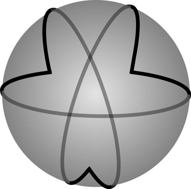
(b)

Figure 1. A planar stick diagram and a spherical stick diagram of a trefoil.

We consider another invariant based on constructing diagrams of knots on the sphere instead of in the plane.

Definition 1.4.

A spherical stick diagram of $[K]$ is a closed curve on the sphere constructed from great circle arcs, with crossing information assigned to each self-intersection, that represents $[K]$. The spherical stick index $\operatorname{ss}[K]$ of a knot type is the minimum number of great circle arcs required to construct a spherical stick diagram of $[K]$.

Remark 1.5.

We could define the spherical stick index of the unknot to be either $1$ or $2$, depending on whether we allow entire great circles in spherical stick diagrams. As such, we leave $\operatorname{ss}[\mbox{Unknot}]$ undefined. If we were to consider the spherical stick indices of links, the choice would become important.

Figure 1b shows a spherical stick diagram of a trefoil. A spherical stick diagram can be obtained via radial projection of a stick knot in space onto a sphere from some point in space, or via radial projection of a planar stick diagram from some point not in the plane.

In Section 2, we establish bounds for the planar stick index in terms of other invariants, including crossing number, stick index, and bridge index. Section 3 establishes similar bounds for the spherical stick index.

In Section 4, we construct planar stick diagrams and spherical stick diagrams for torus knots and compositions of trefoils, providing upper bounds for the planar stick index and spherical stick index of these knot types. In some cases, the bounds from Sections 2 and 3 show that the constructions are minimal.

Our results are as follows. Let $T_{p,q}$ denote the $(p,q)$-torus knot.

Theorem 1.6.

Let $2\leq p<q$. Then

$$\operatorname{pl}[T_{p,q}] \leq 2q-1 \textrm{if}\quad q<2p,$$

$$\operatorname{pl}[T_{p,q}] \leq q \textrm{if}\quad 2p<q,$$

$$\operatorname{pl}[T_{p,q}] \geq 2p+1 \textrm{for all }p.$$

When $q=p+1$ or $q=2p+1$, the inequalities exactly determine the planar stick index to be $\operatorname{pl}[T_{p,p+1}]=\operatorname{pl}[T_{p,2p+1}]=2p+1$.

Theorem 1.7.

Let $2\leq p<q$. Then

$$\operatorname{ss}[T_{p,q}]\leq q.$$

Moreover, $\operatorname{ss}[T_{q-1,q}]=q$.

Let $nT$ denote a composition of $n$ trefoils (of any combination of handedness), and $aT_{L}\#bT_{R}$ denote the composition of $a$ left-handed trefoils with $b$ right-handed trefoils. Because composition of knots is commutative and associative (see [Ada94]), $aT_{L}\#bT_{R}$ is well-defined.

Theorem 1.8.

For $n\geq 1$, $\operatorname{pl}[nT]=2n+3.$

Theorem 1.9.

For $m\geq 1$, $\operatorname{ss}[mT_{L}\#mT_{R}]\leq 2m+2.$

More generally, for $0\leq m<n$, $\operatorname{ss}[mT_{L}\#nT_{R}]=\operatorname{ss}[nT_{L}\#mT_{R}]\leq 2n+1.$

The difference between Theorems 1.8 and 1.9 is striking: the planar stick index of a composition of trefoils is independent of the handedness of the trefoils composed, while our construction of a spherical stick diagram depends heavily on handedness. It would be interesting to know if the bounds in Theorem 1.9 are sharp, and whether the spherical stick index of a composition of trefoils depends on handedness in general. This seems difficult to prove, since most invariants that we could use to obtain lower bounds do not detect handedness of composites. However, by classifying all knots with $\operatorname{ss}[K]\leq 4$ (as we do in Section 5), we can prove that the bound in Theorem 1.9 is sharp in the case of composing two trefoils.

Theorem 1.10.

The nontrivial knot types with $\operatorname{ss}[K]\leq 4$ are

$$3_{1},4_{1},5_{1},5_{2},6_{1},6_{2},6_{3},7_{4},8_{18},8_{19},8_{20},$$

and the square knot $T_{L}\#T_{R}$. All of these knots except the trefoil $3_{1}$ have $\operatorname{ss}[K]=4$.

Corollary 1.11.

$\operatorname{ss}[T_{L}\#T_{R}]=4$, while $\operatorname{ss}[T_{L}\#T_{L}]=\operatorname{ss}[T_{R}\#T_{R}]=5$.

We also see a very unusual characteristic for a naturally defined physical knot invariant:

Corollary 1.12.

There exist nontrivial knots $K_{1}$ and $K_{2}$ so that

$$\operatorname{ss}[K_{1}\#K_{2}]=\operatorname{ss}[K_{1}].$$

2. Planar Stick Index

In general, the planar stick index of a knot is difficult to compute. It is straightforward to construct a planar stick diagram, but hard to prove that it is minimal. In this section, we establish bounds on the planar stick index of a knot in terms of other invariants. These bounds enable us to compute exact values for planar stick index for certain categories of knots in Section 4.

Theorem 2.1.

$\operatorname{pl}[K]\leq\operatorname{s}[K]-1$.

Proof.

Consider a polygonal conformation of $[K]$ that realizes the stick index. If we project the knot onto a plane normal to one stick, that stick projects to a single point. In the “generic case,” the resulting polygonal curve in the plane is a diagram of $[K]$ with at most $s[K]-1$ edges. The diagram fails to be generic if three edges intersect at the same point, or if a vertex overlaps an edge. In such a case, however, we can tweak the original conformation slightly so that after projecting, we obtain a generic $(s[K]-1)$-edge diagram of $[K]$. ∎

Theorem 2.2.

Let $\operatorname{cr}[K]$ be the crossing number of $[K]$. Then

$$\frac{3+\sqrt{9+8\operatorname{cr}[K]}}{2}\leq\operatorname{pl}[K].$$

Proof.

Consider a planar stick diagram of $[K]$ with $n=\operatorname{pl}[K]$ sticks. Each stick can cross at most $n-3$ other sticks, since it can cross neither itself nor the two adjacent sticks. The total number of self-intersections (which is at least $\operatorname{cr}[K]$) is bounded above by $\frac{1}{2}n(n-3)$. Rearranging $\operatorname{cr}[K]\leq\frac{1}{2}n(n-3)$ gives the desired inequality. ∎

Theorem 2.3.

If $K_{1}\#K_{2}$ is the composition of two knots $K_{1},K_{2}$, then

$$\operatorname{pl}[K_{1}\#K_{2}]\leq\operatorname{pl}[K_{1}]+\operatorname{pl}[K_{2}]-2.$$

Proof.

Consider planar stick diagrams for $K_{1}$ and $K_{2}$ that realize planar stick index. Since any two adjacent sticks in the diagram of $K_{1}$ are non-parallel, we can perform an orientation-preserving linear transformation that makes two adjacent sticks of $K_{1}$ perpendicular. We do likewise for the diagram of $K_{2}$.

Once we have these diagrams, we can rotate and attach them at the right angles such that the incident sticks line up. The point at which the corners were attached then becomes a crossing. If $K_{1}$ and $K_{2}$ do not overlap, the resultant diagram is a $(\operatorname{pl}[K_{1}]+\operatorname{pl}[K_{2}]-2)$-stick representation of $K_{1}\#K_{2}$.

If $K_{1}$ and $K_{2}$ do overlap, first note that if necessary we can tweak the diagrams slightly so that the new diagram is generic. We can then choose the new crossings so that sticks from $K_{1}$ always cross over sticks from $K_{2}$. It is clear that the diagram represents $K_{1}\#K_{2}$. ∎

We get another bound on the planar stick index in terms of the bridge index. Let $\operatorname{b}(K,p)$ be the number of local maxima of a knot conformation $K$ relative to a direction (taken to be a vector $p$ on the 2-sphere $S^{2}$). The bridge index is given by

$$\operatorname{b}[K]=\min_{K\in[K]}\min_{p\in S^{2}}\operatorname{b}(K,p).$$

This definition is similar to Milnor’s definition of crookedness (see [Mil50]). However, if an extremum occurs at an interval of constant height, we count it as one extremum rather than infinitely many.

Theorem 2.4.

$2\operatorname{b}[K]+1\leq\operatorname{pl}[K]$

Proof.

For a planar stick diagram, the total curvature is the sum of the exterior angles. There are $\operatorname{pl}[K]$ vertices in a minimal planar stick diagram of a knot $[K]$. Since each vertex has an exterior angle strictly less than $\pi$, the total curvature of such a diagram is less than $\pi\operatorname{pl}[K]$.

We view this diagram as a curve in a plane in 3-space. Bending the sticks slightly out of the plane at each crossing yields a conformation of the knot (as opposed to a diagram). Since we can bend the sticks by an arbitrarily small amount, the final total curvature can be made arbitrarily close to the original total curvature. Since the original total curvature was strictly less than $\pi\operatorname{pl}[K]$, the final total curvature can be made to be less than $\pi\operatorname{pl}[K]$.

Milnor showed in [Mil50] that for any conformation $K$ with total curvature $\operatorname{tc}(K)$,

$$2\pi\operatorname{b}[K]<\operatorname{tc}(K).$$

Since $\operatorname{tc}(K)<\pi\operatorname{pl}[K]$, we find $2\operatorname{b}[K]<\operatorname{pl}[K]$. Since both quantities are integers, the result follows. ∎

3. Spherical Stick Index

Figure 2. A spherical stick trefoil and its stereographic projection.

When studying spherical stick diagrams, it is helpful to consider their stereographic projections. Given a diagram of a knot on a sphere, we choose a point on the sphere not on the diagram to label $\infty$. Consider this the north pole. The stereographic projection relative to this point maps $S^{2}\backslash\{\infty\}$ homeomorphically to $\mathbb{R}^{2}$, which is the plane though the equator, and transfers the diagram into $\mathbb{R}^{2}$. Moreover, stereographic projection preserves the knot type of a diagram. See Figure 2 for an example. The following fact can be proved relatively easily.

Fact 3.1.

Stereographic projection gives a one-to-one correspondence between great circles on the sphere that do not pass through infinity, and circles in the plane that have a diameter with endpoints $p,q$ that contains the origin, and satisfies $|p|\cdot|q|=1.$

In some situations, it is more convenient to think about circles in the plane rather than great circles on the sphere. Most of our figures of spherical stick diagrams will be stereographic projections for clarity.

We prove bounds on spherical stick index, many of which are analogous to those proven in Section 2 for planar stick index.

Theorem 3.2.

$\operatorname{ss}[K]\leq\operatorname{pl}[K]$.

Proof.

Observe that given a polygonal curve in space, radial projection onto a sphere maps each edge to a great circle arc.

Consider a planar stick diagram that realizes planar stick index for $[K]$. We put it in space in a plane not containing the origin and radially project to the unit sphere. The diagram projects to a spherical stick diagram of $[K]$ with $\operatorname{pl}[K]$ great circle arcs. ∎

Theorem 3.3.

$\operatorname{ss}[K]\leq\operatorname{s}[K]-2$.

Proof.

Consider a minimal stick realization of a knot in space. Using a similar trick as appears in [Cal01], we choose a vertex $v$ of the knot, and radially project the knot (minus $v$) onto a sphere centered at $v$. Radial sticks project to points, and non-radial sticks project to great circle arcs. Since the two sticks adjacent to $v$ are radial, the projection has at most $s[K]-2$ arcs. However, it is no longer a closed curve, as there are two “loose ends” corresponding to the sticks incident at $v$.

As projections of line segments, the great circle arcs must be strictly smaller than $\pi$ radians. Since any pair of distinct great circles intersect at two antipodal points, and each arc traverses less than half of a great circle, no two arcs can intersect more than once. In particular, the arcs with “loose ends” intersect at most once. We extend these arcs until they meet, making the extended arcs understrands at any newly-created crossings (to preserve the knot type). This yields a spherical stick diagram of the knot with $\operatorname{s}[K]-2$ arcs. ∎

Theorem 3.4.

$1+\sqrt{1+\operatorname{cr}[K]}\leq\operatorname{ss}[K]$.

Proof.

Consider a spherical stick diagram of $[K]$ with $n=\operatorname{ss}[K]$ great circle arcs. No arc intersects itself, and each arc intersects each of the other $n-1$ arcs at most twice. Also, vertices connecting arcs at endpoints are intersections, but are not crossings in the diagram. Thus, there are at most $2(n-1)-2=2n-4$ crossings on each arc. Since each crossing occurs on exactly two arcs, there are at most

$$\frac{1}{2}n(2n-4)=n(n-2)$$

crossings in the diagram, so $\operatorname{cr}[K]\leq\operatorname{ss}[K](\operatorname{ss}[K]-2)$. Solving for $\operatorname{ss}[K]$ gives the desired inequality. ∎

Theorem 3.5.

$\operatorname{ss}[K_{1}\#K_{2}]\leq\operatorname{ss}[K_{1}]+\operatorname{ss}[K_{2}]$.

Proof.

Suppose we have minimal spherical stick diagrams of $K_{1}$ and $K_{2}$ on the sphere. We position them so that two vertices of the diagrams overlap as shown in Figure 3a. Note that the diagrams may overlap in many other places. As before, we move $K_{2}$ to ensure that the diagram is generic, and choose the new crossings so that arcs in $K_{1}$ cross above arcs in $K_{2}$. We then change the diagrams as shown in Figure 3b to obtain a diagram of $K_{1}\#K_{2}$. Our new diagram has $\operatorname{ss}[K_{1}]+\operatorname{ss}[K_{2}]$ great circle arcs. ∎

(a)

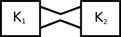
(b)

Figure 3. Composition of spherical stick diagrams. Great circle arcs appear locally as straight lines.

We can bound spherical stick index in terms of an invariant related to the bridge index. Using $\operatorname{b}(K,p)$ as previously defined, we let the superbridge index of a knot $[K]$ be

$$\operatorname{sb}[K]=\min_{K\in[K]}\max_{p\in S^{2}}\operatorname{b}(K,p),$$

as in [Kui87]. The strict inequality $\operatorname{b}[K]<\operatorname{sb}[K]$ holds for all knot types, as proven in [Kui87].

Theorem 3.6.

$\frac{2}{3}\operatorname{sb}[K]+\frac{1}{3}\leq\operatorname{ss}[K]$.

Proof.

Consider a spherical stick diagram of $[K]$ with $n=\operatorname{ss}[K]$ great circle arcs. We modify it as follows to obtain a conformation $K$ in space. For any crossing of the diagram, there is an “overstrand” and an “understrand”, relative to the outside of the sphere. We remove a small portion of the understrand, replacing it with a straight line. We do this for all crossings, and obtain a conformation of $[K]$ that radially projects to our diagram. The conformation consists of $n$ almost-circular arcs, like those in Figure 4.

Given a direction $p\in S^{2}$, we want an upper bound on the number of extrema in the direction $p$. Each of the $n$ points connecting two almost-circular arcs can be an extremum. Other extrema must occur on the interiors of the arcs, and each arc can have at most two interior extrema (see Figure  4). Thus $K$ has at most $3n$ extrema in the direction $p$. Since $\operatorname{b}(K,p)$ counts the number of maxima, $\operatorname{b}(K,p)\leq 3n/2$. Therefore,

$$\operatorname{sb}[K]\leq\max_{p\in S^{2}}\operatorname{b}(K,p)\leq\frac{3n}{2}=\frac{3}{2}\operatorname{ss}[K].$$

Rearranging gives $\frac{2}{3}\operatorname{sb}[K]\leq\operatorname{ss}[K]$.

To improve the bound by $1/3$, we use a small trick that guarantees an arc of length less than $\pi$. We stereographically project our original spherical stick diagram from a point not in the diagram whose antipode is in the diagram. We get a diagram in the plane consisting of circles and one line segment through the origin. We scale the diagram so the line segment is contained in the unit disc, and then stereographically project back to the sphere. The result is a spherical diagram of $[K]$ with one great circle arc of length less than $\pi$, and $n-1$ other circular arcs (not necessarily great circle arcs). We change these into almost-circular arcs to obtain a conformation $K$, and apply the same counting argument as before. Because the great circle arc of length less than $\pi$ can have at most one interior extremum, we find

$$\operatorname{sb}[K]\leq\frac{3\operatorname{ss}[K]-1}{2},$$

which rearranges to the desired inequality. ∎

Since bridge number is known for many more knots than is superbridge number, we note that Kuiper’s result that $\operatorname{b}[K]<\operatorname{sb}[K]$ implies:

Corollary 3.7.

$\frac{2}{3}\operatorname{b}[K]+1\leq\operatorname{ss}[K]$.

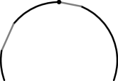
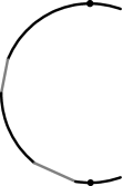
Figure 4. Almost-circular arcs from the proof of Theorem 3.6

Remark 3.8.

In all cases where we know both the superbridge index and spherical stick index, $\operatorname{sb}[K]\leq\operatorname{ss}[K]$. It would be interesting to know whether this holds in general, as it would prove that some of the constructions in the next section realize spherical stick index. (See Remarks 4.2 and 4.4.)

4. Examples

4.1. Torus Knots

Armed with bounds on planar and spherical stick indices, we examine some classes of knots, and prove Theorems 1.6, 1.7, 1.8, and 1.9 stated in the introduction. We begin with the torus knots, one of the most easily described and exhaustively studied classes of knots.

We need a few well-known properties of torus knots. It is known that for any $p$ and $q$, the $(p,q)$-torus knot is equivalent to the $(q,p)$-torus knot (see [Ada94]). So, without loss of generality, we always assume $p<q$. Also, we require $p$ and $q$ to be coprime (otherwise we get a torus link with $\gcd(p,q)$ components).

We need the values of some invariants of $T_{p,q}$ (for $p<q$). First, the bridge index has been shown (see [Sch54] or [Kui87]) to be

$$\operatorname{b}[T_{p,q}]=p.$$

It was shown in [Mur91] that the crossing number is

$$\operatorname{cr}[T_{p,q}]=(p-1)q.$$

Finally, it was proven in [Jin97] that, for $q<2p$,

$$\operatorname{s}[T_{p,q}]=2q.$$

We prove Theorems 1.6 and 1.7, which pertain to planar and spherical stick indices of torus knots.

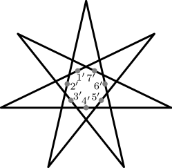
(a)

(b)

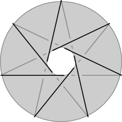
(c)

Figure 5. Construction of $T_{3,7}$ with 7 sticks.

Proof of Theorem 1.6.

Two of the inequalities follow directly from theorems established in Section 2 and the facts above. We can apply Theorem 2.1 to show that when $q<2p$,

$$\operatorname{pl}[T_{p,q}]\leq 2\operatorname{s}[K]-1=2q-1.$$

Similarly, Theorem 2.4 gives

$$\operatorname{pl}[T_{p,q}]\geq 2\operatorname{b}[T_{p,q}]+1=2p+1.$$

It remains to show that for $2p<q$ we can construct a planar stick diagram of $T_{p,q}$ with $q$ sticks. We consider $q$ evenly spaced points on a circle, $z_{1}\ldots z_{q}$, labeled counterclockwise. We then draw $q$ line segments, connecting $z_{n}$ to $z_{n+p}$ for each $n$. The result is a $q$-pointed star, as in Figure 5a. We label the stick from $z_{n}$ to $z_{n+p}$ as stick $n$ (and take these labels modulo $q$). We label the midpoint of stick $n$ as $n^{\prime}$. We can see that the middle of the diagram is a regular $q$-gon for which the midpoint of each side is some $n^{\prime}$.

By construction, stick $n$ attaches to stick $n+p$, which attaches to stick $n+2p$, and so on. Since $p$ and $q$ are coprime for torus knots, the $q$ sticks form a single closed curve. Furthermore, stick $n$ and stick $m$ cross if and only if $m$ is in the following set (modulo $q$)

$$\{n-p-1,\ldots,n-1,n+1,\ldots,n+p-1\}.$$

In this case, we let $I_{m,n}=I_{n,m}$ denote the point of intersection. For each stick, we define directions of “clockwise” and “counterclockwise” relative to the origin. On stick $n$, the intersections $I_{n,n-1},\ldots,I_{n,n-p+1}$ are clockwise from $n^{\prime}$, and $I_{n,n+1},\ldots,I_{n,n+p-1}$ are counterclockwise from $n^{\prime}$ (see Figure  5). This means our diagram has $(p-1)q$ intersections, which is equal to the crossing number of the standard projection of $T_{p,q}$.

We specify the crossings by letting stick $n$ be the overstrand for the $p-1$ crossings clockwise from $n^{\prime}$, and the understrand for the $p-1$ crossings counterclockwise from $n^{\prime}$ (see Figure 5b).

From Figure 5c, we can see our diagram is a projection of a knot on the standard torus in $\mathbb{R}^{3}$. This knot winds around the torus $p$ times in one direction and $q$ times in the other, so it is $T_{p,q}$. ∎

Remark 4.1.

The fact that $\operatorname{pl}[T_{p,p+1}]=\operatorname{pl}[T_{p,2p+1}]=2p+1$ is striking. We suspect, but have not been able to prove, that $\operatorname{pl}[T_{p,q}]=2p+1$ whenever $p+1\leq q\leq 2p+1$.

Figure 6. Seven great circles evenly spaced, for construction of 7-stick spherical projective stick diagrams of $T_{p,7}$

Proof of Theorem 1.7.

To show $\operatorname{ss}[T_{p,q}]\leq q$, we use a similar construction as we used in the previous proof. We begin with a regular $q$-gon on the sphere, centered at the north pole. We extend the sides to great circles. The stereographic projection is shown for $q=7$ in Figure 6. We label the circles counterclockwise from $C_{1}$ to $C_{q}$. We let the basepoint of each circle be the farthest point on the circle from the origin (under the stereographic projection) and label it $1$ through $q$ as in the figure, and label the point antipodal to the basepoint $n$ as $n^{\prime}$. As before, we consider these labels modulo $q$.

Next, we establish some facts about intersections of the circles. Any two great circles in the sphere intersect twice, at antipodal points. (The intersections are no longer antipodal under stereographic projection.) If we fix a circle $C_{n}$ in our diagram, any other circle $C_{m}$ intersects it once clockwise from $n$ and once counterclockwise from $n$. Furthermore, an intersection point of circles $C_{m}$ and $C_{n}$ that is clockwise from $n$ must be counterclockwise from $m$. Hence for any $m\neq n$, there is a unique intersection $i_{m,n}$ of circle $C_{m}$ and circle $C_{n}$ so that $i_{m,n}$ is counterclockwise from $m$ and clockwise from $n$.

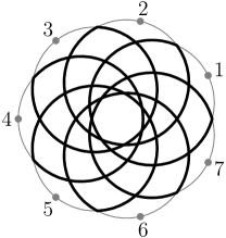
(a)

(b)

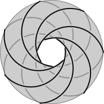
(c)

Figure 7. Construction of $T_{6,7}$ with $7$ great circle arcs.

We construct a diagram by using an arc $a_{n}$ from each great circle $C_{n}$. For circle $C_{n}$, we use the arc that starts at $i_{n,n-p}$ and goes counterclockwise to $i_{n+p,n}$. The diagram for $T_{6,7}$ is shown in Figure  7a.

We can connect these arcs to form a closed loop by the same argument as in the previous proof, using the fact that $p$ and $q$ are coprime. Furthermore, for each $n$, the $2(p-1)$ points contained in the interior of arc $a_{n}$,

$$i_{n,n-p+1},\ldots,i_{n,n-1},i_{n+1,n},\ldots,i_{n+p-1,n},$$

are all intersections of this curve with itself. To see this, note that an intersection of two circles $C_{n}$ and $C_{m}$ is equidistant from $n$ and $m$. Again, we get a diagram with $(p-1)q$ intersections.

We choose the crossings for our diagram by letting arc $a_{m}$ be the overstrand for the $p-1$ crossings counterclockwise from $m$ and the understrand for the $p-1$ crossings counterclockwise from $m^{\prime}$ (see Figure  7b). We can then construct a conformation of $T_{p,q}$ that projects to our diagram, as in Figure 7c.

To show that $\operatorname{ss}[T_{q-1,q}]\geq q$ (and hence $\operatorname{ss}[T_{q-1,q}]=q$), we note that $\operatorname{cr}[T_{q-1,q}]=(q-2)q$, and apply the lower bound of Theorem 3.4. ∎

Remark 4.2.

If the bound $\operatorname{sb}[K]\leq\operatorname{ss}[K]$ were to hold, the fact that $\operatorname{sb}[T_{p,q}]=\min\{2p,q\}$ (see [Kui87]) would imply $\operatorname{ss}[T_{p,q}]=q$ for $p<q<2p$.

4.2. Compositions of Trefoil Knots

Another class of knots that we will examine is the set of compositions of trefoil knots. Adams et al. (see [ABGW97]) computed the stick index of such knots to be

$$\operatorname{s}[nT]=2n+4.$$

We use this result to compute the planar stick index of compositions of trefoils.

Proof of Theorem 1.8.

By [ABGW97] and Theorem 2.1, we know $\operatorname{pl}[nT]\leq\operatorname{s}[nT]-1=2n+3$. Furthermore, it is known (see [Sch54] or [Sch03]) that the bridge index of a composition of knots is given by

$$\operatorname{b}[K_{1}\#K_{2}]=\operatorname{b}[K_{1}]+\operatorname{b}[K_{2}]-1.$$

Since $\operatorname{b}[T]=2$, it follows that $\operatorname{b}[nT]=n+1$, and Theorem 2.4 implies $\operatorname{pl}[nT]\geq 2\operatorname{b}[nT]+1=2n+3$. ∎

When working with compositions of trefoils, we must be aware of a caveat. The trefoil knot is invertible, so there is a unique composition of two given trefoil knots. However, since the trefoil is chiral, we must make a distinction between left-handed and right-handed trefoil knots in compositions. For example, the square and granny knots are the two distinct compositions of two trefoils (see Figure 8). The $2n+4$-stick construction of $nT$ is independent of handedness (as discussed in [ABGW97]), so this distinction does not affect Theorem 1.8.

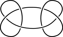
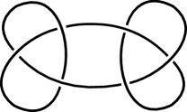
Figure 8. The square knot $T_{L}\#T_{R}$ and the granny knot $T_{R}\#T_{R}$.

The bulk of the proof of Theorem 1.9 is in the following lemma:

Lemma 4.3.

If $m>0$, we have

$$\operatorname{ss}[mT_{L}\#mT_{R}] \leq 2m+2,$$

$$\operatorname{ss}[(m+1)T_{L}\#mT_{R}] \leq 2m+3,$$

$$\operatorname{ss}[mT_{L}\#(m+1)T_{R}] \leq 2m+3.$$

Proof.

We use the same conventions and notation as in the proof of Theorem 1.7 and demonstrated in Figure 6. We start with $q$ great circles spaced symmetrically around the north pole, and label them from $C_{1}$ to $C_{q}$ counterclockwise. We assume throughout that $q>2m+1$. We define the basepoint of circle $C_{r}$ as its farthest point from the origin, labelled $r$ and the point $r^{\prime}$ as its closest point to the origin. Let $i_{r,s}$ denote the intersection of circles $C_{r}$ and $C_{s}$ that is counterclockwise from $r$ and clockwise from $s$. Again, consider all labels modulo $q$.

Let $k$ be an integer, and $m=\lfloor k/2\rfloor$. Then, we will prove the following set of statements for all $k$:

For odd $k$, we have:

1. There is a diagram using $k+2$ arcs of circles that represents $(m+1)T_{L}\#mT_{R}$.

2. The diagram uses one arc from each circle corresponding to $-m,\ldots,m+2$, and we can pick an orientation on the diagram so that the circles are traversed in this order.

3. If an arc of circle $C_{r}$ is in the diagram, it contains point $r^{\prime}$ but not the basepoint.

4. The vertices of the diagram are $i_{r,r+1}$ for $p\in\{-m,\ldots,m+1\}$, along with $i_{m+2,-m}$.

5. Arc $a_{m+2}$ is the overstrand in all of its crossings except for the crossing with arc $a_{-m}$.

For even $k$, we have:

1. There is a diagram using $k+2$ arcs of circles that represents $mT_{L}\#mT_{R}$.

2. The diagram uses one arc from each circle corresponding to $-m,\ldots,m+1$, and we can pick an orientation so that the circles are traversed in this order.

3. If an arc of circle $C_{r}$ is in the diagram, it contains point $r^{\prime}$ but not the basepoint.

4. The vertices of the diagram are $i_{r,r+1}$ for $p\in\{-m,\ldots,m\}$, along with $i_{m+1,-m}$.

5. Arc $a_{-m}$ is the overstrand in all of its crossings except for the crossing with arc $a_{m+1}$.

We start with the base case, $k=1$. We connect the three vertices $i_{1,2}$, $i_{2,q}$, and $i_{2,1}$ via arcs on circles corresponding to $1,2,q$ that pass through points $1^{\prime},2^{\prime},q^{\prime}$ respectively. This yields a three-crossing diagram, and by choosing crossings appropriately we obtain a left-handed trefoil that satisfies the conditions of the $k=1$ case of our induction hypothesis. The $q=7$ case is shown in Figure 9, and the picture looks similar for other $q$.

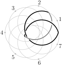
(a)

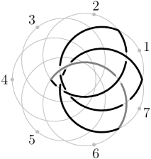
(b)

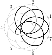
(c)

Figure 9. Demonstrating the base case and the inductive step in the proof of Lemma 4.3, with $n=7$. We go from the $k=1$ case to $k=2$ to $k=3$.

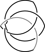
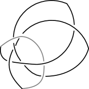
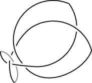
Figure 10. Demonstrating how the newly added arc can be modified via isotopy to reveal a composed trefoil.

Suppose that the inductive hypotheses hold for some odd $k<q$. By assumption, we have a diagram of $(m+1)T_{L}\#mT_{R}$ using arcs corresponding to $-m,\ldots,m+2$. We modify our diagram by extending arc $a_{m+2}$ clockwise from $i_{m+1,m+2}$ to $i_{m+2,-m-1}$ and arc $a_{-m}$ clockwise from $i_{-m+1,-m}$ to $i_{-m-1,-m}$. We then add an arc of circle $C_{-m-1}$, which goes clockwise from $i_{m+2,-m-1}$ to $i_{-m-1,-m}$. Conditions (2) and (3) guarantee the new arcs of circles $C_{m+2}$ and $C_{-m}$ are extensions of the old ones. Conditions ($2^{\prime}$), ($3^{\prime}$), and ($4^{\prime}$) of the $k+1$ case immediately follow (see Figure 9).

We must specify the crossings for our new diagram. We keep all crossings from the original diagram. We let arc $a_{-m}$ be the overstrand at $i_{m+2,-m}$, arc $a_{m+2}$ be the overstrand at $i_{-m-1,m+2}$, and arc $a_{-m-1}$ be the overstrand at all of its other crossings (see Figure  9). By construction, condition ($5^{\prime}$) is satisfied for the $k+1$ case.

It remains to show that condition ($1^{\prime}$) holds. Because arc $a_{-m-1}$ is the overstrand at all crossings except its crossing with arc $a_{m+2}$, and arc $a_{m+2}$ is the overstrand at all crossings except those with arc $a_{-m}$, we can move arc $a_{-m-2}$ as in Figure 10. The result is the composition of a right-handed trefoil and the original diagram. By (1), this is $[(m+1)T_{L}\#mT_{R}]\#T_{R}$. This proves the inductive hypothesis for $k+1$.

Finally, consider the case when $k$ is even. The argument is nearly identical to the previous one. This time, we extend arcs $a_{m+1}$ and $a_{-m-1}$ to the points $i_{m+1,m+2}$ and $i_{m+2,-m-1}$, and connect these points by adding an arc of circle $C_{m+2}$ between them. We set arc $a_{m+2}$ as the overstrand in all of its crossings except that with arc $a_{-m-1}$, and make $a_{m+1}$ the overstrand at $i_{m+1,-m-1}$ (see Figure 9). We can prove conditions (1)-(5) by the same arguments as above. This completes the induction.

Since $q$ is arbitrary, we have shown that $\operatorname{ss}[mT_{L}\#mT_{R}]\leq 2m+2$ and
$\operatorname{ss}[(m+1)T_{L}\#mT_{R}]\leq 2m+3$ hold for all $m$. Reflecting a $2m+3$-arc diagram of $mT_{L}\#(m+1)T_{R}$ yields a $2m+3$-arc diagram of $(m+1)T_{L}\#mT_{R}$, proving the last inequality. ∎

Proof of Theorem 1.9.

It remains to show that for $n>m$,

$$\operatorname{ss}[nT_{L}\#mT_{R}]=\operatorname{ss}[mT_{L}\#nT_{R}]\leq 2n+1.$$

We prove this by induction on $n$. The base case $n=m+1$ was proven in Lemma 4.3. For the inductive step, it suffices to show that given a knot, we can compose it with a trefoil by slightly extending two arcs past a vertex and adding two great circle arcs (see Figure  11). ∎

Remark 4.4.

It would be interesting to know whether the bounds given in Theorem 1.9 are tight. If $\operatorname{sb}[K]\leq\operatorname{ss}[K]$ were to hold, then the bounds of Lemma 4.3 would be tight, but this would not help with the general case.

(a)

(b)

Figure 11. Adding a trefoil at a vertex using two great circle arcs, which locally appear as line segments.

5. Classification of Knots with $\operatorname{ss}=4$.

Our construction in Theorem 1.9 depends on the handedness of the composed trefoils, but this does not imply that spherical stick index depends on handedness. However, we will show that $T_{L}\#T_{R}$ and $T_{L}\#T_{L}$ have different spherical stick indices (see Figure 12). By Theorem 3.4, any knot with at least 4 crossings has $\operatorname{ss}[K]\geq 4$. Combining this with Theorem 1.9 gives $\operatorname{ss}[T_{L}\#T_{R}]=4$ and $\operatorname{ss}[T_{L}\#T_{L}]\leq 5$. To show that $\operatorname{ss}[T_{L}\#T_{L}]=5$, we classify all knots with $\operatorname{ss}[K]\leq 4$.

Figure 12. Spherical projective stick diagrams of the square knot $T_{L}\#T_{R}$ and the granny knot $T_{L}\#T_{L}$ that realize their spherical stick indices.

Proof of Theorem 1.10.

To construct an $\operatorname{ss}$-4 diagram, we start with a configuration of four great circles on the sphere, as in Figure 13. It is not difficult to show that any generic configuration divides the sphere into triangular and quadrilateral regions, and that no two triangles or quadrilaterals can share a side. The only way to do this on a sphere (up to isotopy) is the arrangement shown in Figure 13. Thus, this is the only configuration that we need to consider.

Figure 13. The stereographic projection of an arrangement of four great circles on a sphere.

Given this diagram, we find all ways to form a closed loop out of one arc from each great circle $G_{i}$. We note that the complement of such a closed loop, which consists of all arcs removed from the diagram to obtain the first loop, is itself a closed loop with one arc from each great circle. It will be convenient to describe loops by their complements, because the loops with the most crossings have simple complements.

We choose a closed curve in the diagram. Suppose the complement contains $n$ edges, and hence $n$ vertices. Four of these vertices are the “turning vertices” where the complement switches from one circle to another, and the other $n-4$ are “passing vertices” where the complement passes straight through an intersection. Note that the complement may pass through a single vertex twice, removing all four edges. Thus, at least $\lceil(n-4)/2\rceil$ vertices are passed through. These vertices, along with the 4 turning vertices, are not crossings of the original curve, so the number of remaining crossings is at most

$$12-(4+\lceil(n-4)/2\rceil)=10-\lceil n/2\rceil.$$

Note that for $n>8$, there will be at most five crossings. We will see that we pick up all knots of five or fewer crossings from the complements with $n\leq 6$.

By symmetry, it is not hard to check that all pairs of an edge $e$ and an adjacent vertex $v$ are combinatorially equivalent. Thus, we need only consider complementary loops including $v$ as a turning vertex and containing $e$, as in Figure 13.

By explicitly considering complements constructed from 7 or 8 edges, we can see that they only produce knots of four or fewer crossings. Hence, we can limit consideration to complements of 4, 5, or 6 edges. There are none with 5 edges as any such would need to have two edges on one great circle and one on each of the others, and we cannot close such a complement up. Up to equivalence of diagrams we obtain one complement with four edges and two with six edges, as appear in Figure 14.

We consider all possible crossing choices for the diagrams in Figure 14 and identify what knots result. This list of knots includes all knots of five or fewer crossings. We conclude that the nontrivial knots with $\operatorname{ss}[K]\leq 4$ are

$$3_{1},4_{1},5_{1},5_{2},6_{1},6_{2},6_{3},7_{4},8_{18},8_{19},8_{20},T_{L}\#T_{R}.$$

It follows from Theorem 3.4 that the trefoil has $\operatorname{ss}[K]=3$ and that the other knots listed have $\operatorname{ss}[K]=4$. ∎

Figure 14. The three possible loops with at least $6$ crossings.

$3_{1}$	$4_{1}$	$5_{1}$	$5_{2}$
$6_{1}$	$6_{2}$	$6_{3}$	$7_{4}$
$8_{18}$	$8_{19}$	$8_{20}$	Square Knot

Table 1. Nontrivial knots with $\operatorname{ss}\leq 4$.

Using a computer (with the help of the program Knotscape), we carried out a similar process to classify knots with $\operatorname{ss}[K]=5$. We found that there are $666$ prime knots and $17$ composite knots with $\operatorname{ss}[K]=5$. In particular, we found that all knots of eight or fewer crossings (prime or composite) have $\operatorname{ss}[K]\leq 5$. The list also includes nine-crossing knots except for $9_{2}$, $9_{3}$, $9_{4}$, $9_{15}$, $9_{18}$, $9_{23}$, $9_{36}$, $4_{1}\#5_{1}$, $4_{1}\#5_{2}$, and $T_{L}\#T_{L}\#T_{L}$ and all ten-crossing nonalternating prime knots except for $10_{152}$ and $10_{154}$.

Since $\operatorname{ss}[T_{L}\#T_{L}\#T_{L}]>5$, spherical stick index distinguishes between the two distinct types of compositions of three trefoils, one consisiting of all left or all right trefoils and one with a mixture of the two. We found a few torus knots with $\operatorname{ss}[T_{p,q}]$ strictly less than $q$: $\operatorname{ss}[T_{2,5}]=4$ and $\operatorname{ss}[T_{2,7}]=\operatorname{ss}[T_{2,9}]=5$. Note that these knots still satisfy $\operatorname{sb}[K]\leq\operatorname{ss}[K]$, as $\operatorname{sb}[T_{p,q}]=\min\{2p,q\}$ is $4$ in these cases.

Proof of Corollary 1.12.

From above, $\operatorname{ss}[T_{L}\#T_{L}]=\operatorname{ss}[T_{L}\#T_{L}\#T_{R}]=5$. ∎

References

- [ABGW97] Colin Adams, Bevin Brennan, Deborah Greilsheimer, and Alexander Woo. Stick numbers and composition of knots and links. J. Knot Theory Ramifications, 6(2):149–161, 1997.
- [Ada94] Colin Adams. The Knot Book. W. H. Freeman and Company, 1994.
- [AS09] Colin Adams and Todd Shayler. The projection stick number of knots. J. Knot Theory Ramifications, 18(7):889–899, 2009.
- [Cal01] Jorge Calvo. Geometric knot spaces and polygonal isotopy. J. Knot Theory Ramifications, 10(2):245–267, 2001.
- [Jin97] Gyo Taek Jin. Polygon indices and superbridge indices of torus knots and links. J. Knot Theory Ramifications, 6(2):281–289, 1997.
- [Kui87] Nicolaas Kuiper. A new knot invariant. Math. Ann., 278(1-4):193–209, 1987.
- [Mil50] John Milnor. On the total curvature of knots. The Annals of Mathematics, 52:248–257, 1950.
- [Mur91] Kunio Murasugi. On the braid index of alternating links. Trans. Amer. Math. Soc., 326(1):237–260, 1991.
- [Sch54] Horst Schubert. Über eine numerische Knoteninvariante. Mathematische Zeitschrift, 61:245–288, 1954.
- [Sch03] Jennifer Schultens. Additivity of bridge numbers of knots. Math. Proc. Cambridge Philos. Soc., 135:539–544, 2003.