Electron velocity distribution instability in magnetized plasma wakes and artificial electron mass

Abstract

The wake behind a large object (such as the moon) moving rapidly through a plasma (such as the solar wind) contains a region of depleted density, into which the plasma expands along the magnetic field, transverse to the flow. It is shown here that (in addition to any ion instability) a bump-on-tail which is unstable appears on the electrons’ parallel velocity distribution function because of the convective non-conservation of parallel energy. It arises regardless of any non-thermal features on the external electron velocity distribution. The detailed electron distribution function throughout the wake is calculated by integration along orbits; and the substantial energy level of resulting electron plasma (Langmuir) turbulence is evaluated quasilinearly. It peaks near the wake axis. If the mass of the electrons is artificially enhanced, for example in order to make numerical simulation feasible, then much more unstable electron distributions arise; but these are caused by the unphysical mass ratio.

1 Introduction

Magnetized plasma wakes have attracted renewed interest recently because of new measurements of the solar wind in the vicinity of the moon [1, 2], but also because of their wider applications to space-craft, dust grains, and laboratory flow measurement probes [3, 4]. This paper explores the effects of supersonic wakes on electron parallel-velocity distributions and the instability that is induced.

We consider an insulating object whose size, $R$, is much greater than the Debye length, $\lambda_{De}=\sqrt{\epsilon_{0}T_{e}/e^{2}n_{e}}$, so that with the exception of a negligible thickness sheath, the surrounding region can be considered quasi-neutral. We suppose that the object is moving through a magnetized plasma in which the ion Larmor radius is also much smaller than $R$. The dynamics parallel to the magnetic field can then be separated from the perpendicular for the ions and even more definitively for the electrons (whose Larmor radius is even smaller). This situation is very representative, for example, of the moon and other unmagnetized planetary bodies moving through the solar wind. The moon’s radius is 1730km; the Debye length is of order 10m and the ion Larmor radius of order 40km[5, 6]. Although the solar wind has ratio of plasma to magnetic pressure, $\beta\sim 1$, and thus the wake experiences significant magnetic perturbations (of order 10% at 4 moon radii [2]), these will be ignored. The magnetic field here is taken to be uniform and simply one-dimensionalizes the problem. Many other Alfvénic phenomena must be accounted for if non-zero beta effects are to be incorporated (see e.g. [7, 8]), but we here focus on the electrostatic phenomena, which are an important part of the picture.

We will assume for simplicity during the development that the direction of object motion, or equivalently, in the frame of the object, the plasma drift, is at right angles to the magnetic field. It is shown in section 6, how the results we obtain can immediately, rigorously, be generalized and applied to oblique field-drift alignment, which is more typical of the solar wind.

In the rest-frame of the object, the electrons and ions sweep rapidly past under the influence of a drift electric field perpendicular to both the magnetic field and plasma drift velocity $v_{\perp}$. Typical solar wind velocity is of order 400km/s, roughly ten times the ion sound speed.

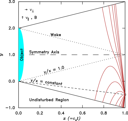
Figure 1: Geometry of a wake, illustrating electron orbits (curves) tracked back from position (1,0.5), and self similar lines ($y/x=const$) on which the potential is constant.

Fig. 1 illustrates the geometry of a wake in which the spatial coordinate in the drift direction ($x$) has been divided by $v_{\perp}/c_{s}$, where $c_{s}$ ($=\sqrt{T_{e}/m_{i}}$ for a Maxwellian) is the (cold ion) sound speed. Thus $dx$ is equal to $c_{s}dt$ when moving at the constant speed $v_{\perp}$. In these units the object is foreshortened by a ratio equal to the perpendicular Mach number and its wake $x$-extent is approximately equal to its radius. We will assume the drift Mach number is large enough to justify ignoring the object’s radius of curvature at its edges. This is the only place where the treatment is limited to supersonic cases. Subsonic flow gives rise to object elongation in this scaled coordinate system, and its curvature cannot then safely be ignored (unless it starts as a flat disk rather than a sphere). Note, though, that the mechanisms we explore are still active in subsonic cases, even though our quantitative treatment cannot be expected to be accurate.

The physics close to the edge of the object, before particle streams from above and below have begun to overlap, is well represented as the expansion of a plasma into vacuum, which has been well understood for a long time [9, 10, 11]. It has also been shown more recently [12] that the additional drifts arising from self-consistent electric field in the magnetized case can be ignored, reducing the problem to two dimensions. Using quasineutrality, $n_{e}=n_{i}$, the ion dynamics can be solved self-consistently, analytically by ignoring the ion pressure or numerically in one dimension with full ion kinetics [9, 13], and taking the potential to be given by a direct relationship with the electron density such as the Boltzmann relation $n_{e}\propto\exp(e\phi/T_{e})$, or more generally a polytropic assumption [14, 15] $p_{e}\propto n_{e}^{\gamma}$.

To justify these simple electron models one invokes (1) Liouville’s theorem that, if collisionless, the electron distribution function is constant on an orbit, and (2) the presumption that all (or nearly all) the electron orbits can be tracked back to the undisturbed plasma. One must also invoke (3) an electron parallel energy conservation equation, normally in the form ${1\over 2}m_{e}v_{\parallel}^{2}-e\phi=constant$, where $m_{e}$ is the electron mass, $v_{\parallel}$ its parallel velocity, $-e$ its charge, and $\phi$ the electric potential. When the external undisturbed parallel distribution function far from the object (where $\phi=0$), is a function only of $v_{\parallel}^{2}$, then with this conservation law, the distribution at a position where the potential $\phi$ is non-zero is also of this form, but appropriately shifted in $v_{\parallel}^{2}$. The result is that if the distribution starts Maxwellian it remains Maxwellian,; and similarly that if it starts having a so-called Kappa distribution [16]

$$f(v)\propto(1+v_{\parallel}^{2}/\kappa\theta^{2})^{\kappa+1},$$ (1)

(which can be considered a generalized Lorentz distribution) then it remains a Kappa distribution with the same $\kappa$ (but varying $\theta$) [17]. A Kappa distribution gives rise to polytropic density variation with $\gamma=1-2/(2\kappa-1)$. In any case the density is a well-defined function of potential, not of position explicitly.

The purpose of this paper is to call out two facts about this approach to one-dimensional (parallel) electron dynamics, and explore their consequences. The first is that energy conservation and Liouville’s theorem guarantee that if the distant unperturbed electron velocity distribution is stable and symmetric (but not otherwise), then the distribution within the wake is also stable. The second is that parallel energy conservation is an approximation, good only to lowest order in the square-root of the electron to ion mass ratio $\sqrt{m_{e}/m_{i}}$. Consequently the stability properties of the electron distribution function are crucially determined by the mass ratio, and finite mass ratio may need to be accounted for.

Moreover, theoretical models that use artificial values of mass ratio closer to unity than in nature, which is common in PIC codes applied to the moon wake [18, 19, 20], will violate parallel energy conservation more strongly, and will lead to more unstable electron distributions in wakes, thus failing to represent actual physics.

It is shown that finite electron mass gives rise routinely to bump-on-tail instability in quasi-neutral magnetized plasma wakes. The quasi-linear strength of the instability is evaluated for different ion to electron mass ratios. For physical values of the ratio (1835 for protons) the energy transferred from unstable electrons to plasma waves is up to $10^{-3}$ of the total energy of the distribution function. This level of instability is may well bear on space-craft observations [21, 1]. For artificial ion to electron mass ratio of 25 (a value not infrequently used in PIC simulations) instability energy fractions roughly 100 times higher occur. These are unphysical.

2 Self-similar potential solution

We briefly summarize the standard self-similar solution arising from the ion dynamics[9, 14, 15]. It serves to set the shape of the potential variation in which the electron dynamics is analysed. Ignoring ion pressure (which is quite well justified even when the external ion temperature is comparable to $T_{e}$ because of the ions’ cooling caused by their acceleration[9]) the ion continuity and (parallel) momentum equations are sufficient. Using the scaled $x$-variable, velocities normalized to the (undisturbed) sound speed, $c_{s}$, and potential in units of $T_{e}/e$, the equations can be solved for Boltzmann density variation to obtain, when $y/x\geq-1$:

$$\phi=-1-y/x\ ;\qquad n=n_{\infty}\exp\phi\ ;\qquad v_{\parallel i}=-\phi\ .$$ (2)

For $y/x<-1$, the potential is undisturbed: $\phi=0$, $n=n_{\infty}$. We use subscript $\infty$ to denote the external, undisturbed values, and we have set the external parallel drift to zero, $v_{\parallel i\infty}=0$. (See section 6 for non-zero $v_{\parallel i\infty}$.)

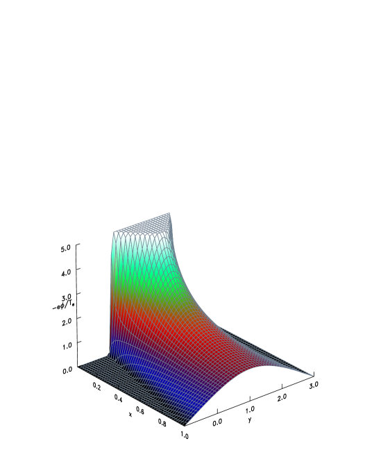
Figure 2: Approximate electron normalized potential energy ($-e\phi/T_{e}$) as a function of position, corresponding to eq. (4)

This self-similar solution, in which parameters are a function only of the ratio $y/x$, holds only to the extent that ions arriving through the wake from the other side of the object can be ignored. The form applies with the substitution $y\rightarrow 2R-y$ (where $R$ is the object’s half-height) to the upper limb of the wake. See Fig 1. At the axis of symmetry, the two opposite ion streams merge. Although the equations are then not rigorously justified, the resultant can be reasonably approximated [9] by taking the density to be the sum of the stream given by eq. (2) plus its equivalent with $y\rightarrow 2R-y$. The resulting potential can quickly be shown to be

$$\phi=-1-R/x+\ln\left[2\cosh\left({R-y\over x}\right)\right].$$ (3)

However, this expression does not exactly go to zero at $y=-x$, so it is better to subtract from it its value at $y=-x$ and use the resulting form:

$$\phi=\ln\left[\cosh\left({R-y\over x}\right)\right]-\ln\left[\cosh\left(R+x\over x\right)\right].$$ (4)

The difference is negligible for $x\ \hbox to0.0pt{\raise 2.58334pt\hbox{$<$}\hss}\lower 2.15277pt\hbox{$\sim$}\ 1$. Fig. 2 is a 3-D rendering of this potential with spatial units scaled so that $R=1$. [In the very far wake, at distances exceeding $Rv_{\perp}/c_{s}$ ($x>1$), some simulations, e.g. [18], indicate a more complicated wake potential structure. We are interested in the nearer wake where the electron instability processes are stronger and the potential structure more robust.]

For analytic convenience, two cruder approximations have also been explored. The “linear $\phi$” is simply to suppose that eq. (2) applies up to the axis of symmetry and the upper solution applies above it; the “flat-top $\phi$” is to adopt eq (2) only until $-\phi$ reaches the value $1+R/x-\ln 2$ and then flat otherwise, in the near-axis region. For these cruder forms the orbit can be integrated analytically which is useful for verification of the numerical orbit solution to be described in section 4.

3 Electron stability with energy conservation

The instability we consider here is that of electrostatic waves arising from the parallel electron distribution function shape. Other possible mechanisms include anisotropy-driven instabilities involving the magnetic field and instability arising from the two-stream nature of the ions, which has been characterized elsewhere[9, 10]. We ignore these other instabilities and focus on the electrostatic electron instability which will be by far the fastest growing, if it exists. The Penrose criterion states that instability arises if and only if there is a minimum in the one-dimensional distribution function $f(v)$ at a velocity $v_{0}$ and that $\int[f(v)-f(v_{0})]/(v-v_{0})^{2}dv>0$ [22]. It therefore suffices for stability to demonstrate that $f(v)$ is monotonically decreasing either side of a single maximum. Maxwellian or Kappa distributions, even with a shift of velocity origin representing parallel drift, are stable by this criterion.

At any point in space, the collisionless electron velocity distribution function at any velocity $v_{\parallel}$ may in principle be found by tracking backwards along the (phase-space) orbit until one arrives somewhere in the unperturbed plasma, where the distribution function at the corresponding energy is known. If such an orbit instead tracks back until it intercepts the object, then under the assumption the object is purely absorbing, that orbit is unpopulated.

Recall, however, that all the orbits move with a constant velocity in the perpendicular direction (in the rest frame of the object). If the typical electron thermal velocity is much larger than this drift velocity, then the spatial trajectory of all the electron orbits will be dominated by parallel motion rather than by the perpendicular drift, and as a result hardly any orbits will actually intercept the object.

In a wake, the electric potential is negative, repelling electrons. The height of the potential energy hill that the electrons encounter, which peaks at the axis of symmetry of the wake, depends upon the $x$-position in the wake. For a point on the negative $y$ side of the wake, orbits with sufficiently negative velocity at the point track backwards over the hill to the upper side of the wake. Others are reflected by the hill (if $v_{y}<0$) and track to the lower side, as illustrated in Fig. 1. Nevertheless, if the distant electron distribution is reflectionally symmetric about the wake axis, and parallel energy is conserved, then it makes no difference which side of the wake the orbit originated from. The electron distribution at the point of interest is then equal to the unperturbed distribution shifted by energy.

If, on the contrary, the distant electron distribution is asymmetric in velocity, for example shifted in velocity, representing a net parallel mean velocity of electrons, the electron distribution in the vicinity of the wake will then possess a discontinuity at the marginal velocity whose orbit only just crosses the potential hill. Higher energy electrons have orbits that are monotonic in $y$ and have arisen from the negative $v_{\parallel}$ part of the distribution in the upper region. Lower energies are reflected orbits that arose from the positive $v_{\parallel}$ part of the distribution function in the lower region. The distribution will have a local minimum if the shift of velocity in the distant distribution is in the negative direction. In other words, if the distribution of electrons that cross the hill (i.e. have negative distant velocity) is larger (at the same energy) than those that are reflected (i.e. have positive distant velocity) instability may arise. [Mathematically the discontinuity is an infinite gradient, but acts as if the sign of $f^{\prime}$ has changed.]

(a)                                                           (b)                                                          

Figure 3: Distribution functions adjacent to a potential energy hill of normalized height $2$, when the external distribution has a velocity shift $v_{S}$. (a) at potential zero, in the unperturbed region; (b) at a position where normalized potential is 0.5. The shape is unstable (bump-on-tail) if $v_{s}<0$.

Fig. 3 illustrates the effect on the distribution function, using a Kappa distribution to emphasize that the effect is not dependent on Maxwellian distributions. The undisturbed electron distribution is taken as $f(v)=[1+(v-v_{s})^{2}/(\kappa\theta^{2})]^{-(\kappa+1)}$ with $\theta=1$, $\kappa=2$, and the conserved energy is ${1\over 2}v^{2}+E_{p}$, where $E_{p}$ is the potential energy in normalized units. The presence of the potential hill forms an unstable distribution at the reflection discontinuity if the distribution’s velocity shift $v_{s}$ is negative, so that reflected electrons (with $v$ immediately above the discontinuity) have a smaller unperturbed distribution function. Postive $v_{s}$ can give rise to a dimple at the top of the distribution function (Fig. 3(a)), but this is unlikely to be Penrose-unstable for small $v_{s}$, and disappears at positions where $E>{1\over 2}v_{s}^{2}$ (Fig. 3(b)).

Asymmetry in the electron distribution is known to arise in the solar wind especially in the form of the “Strahl”, an energetic parallel electron tail flowing away from the sun, believed to arise because of magnetic-mirror force acceleration. However, this population is predominantly at high energies and has a relatively low density; so the instability will saturate at a modest level.

4 Instability from energy-nonconservation

We now consider an effect that can cause instability even when the external electron distribution is reflectionally symmetric. Therefore in this section only unshifted external distribution functions are considered. The effect arises because parallel electron energy is not exactly conserved along orbits. Energy non-conservation can be considered, in the moving frame of the background drift, to arise from the fact that the wake potential is changing with time. Alternatively, in the frame of the object, it comes from the convective perpendicular velocity, and may be understood from the parallel momentum equation in steady state ($\partial/\partial t=0$)

$$v_{\perp}{\partial v_{\parallel}\over\partial x}+v_{\parallel}{\partial v_{\parallel}\over\partial y}={e\over m_{e}}{\partial\phi\over\partial y}\qquad\longrightarrow\qquad{\partial v\over\partial x}+v{\partial v\over\partial y}={1\over m_{r}}{\partial\phi\over\partial y}.$$ (5)

The first form here is the dimensional equation to help the reader with familiarity, the second is the equation expressed in dimensionless units, where $m_{r}=m_{e}/m_{i}$, and the parallel subscript has been dropped for brevity. If the first term on the left hand side of either of these equations were absent, then that side becomes simply ${1\over 2}\partial v^{2}/\partial y$, a total derivative, which leads immediately to the conservation of energy ${1\over 2}v^{2}-\phi/m_{r}=constant$, in normalized units. The extra term means parallel energy is not conserved. The extra term is apparently smaller than the other terms by a factor of order $v_{\perp}/v_{e}$, although we shall see in a moment that the factor is actually $c_{s}/v_{e}=\sqrt{m_{r}}$, but it is not immediately obvious how important it is, and what it actually does to the distribution function.

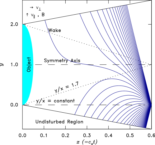
Figure 4: Orbits that all end at the point (0.6,0.) determining the distribution function there. Mass ratio $m_{r}^{-1}=25$.

Heuristically one can understand how a depression in the electron distribution function (and hence an instability) arises as follows. Figure 4 plots a series of actual orbits for illustration. The electron orbits that are most affected by the convective drift are those which spend longest near the peak of the potential (i.e. the symmetry axis). They do so because their parallel velocity is near zero there. These are the marginal orbits that just barely make it over the potential hill or are just barely reflected. They start in the unperturbed region at a parallel speed that has to be high enough to climb the potential hill at a position where the hill is high (because $x$ is smaller). They drift across the field during their time near the potential peak (not gaining parallel energy) to where the potential is lower (because $x$ is larger). Then their evolving parallel speed carries them down the hill to the final position, but as it does so they gain parallel energy corresponding only to the difference between the lower potential peak and the final position. The distribution function at the final position and speed ($f(v)$) is equal to the external distribution function at the starting point with the starting speed ($f_{\infty}(v_{\infty})$), but the starting speed is higher than would be the case with energy conservation. This effect is present for all orbits but it is much stronger for marginal orbits. The distribution function $f$ is therefore smaller for marginal orbits (because their starting speed is higher) than it is for orbits further from marginal. That is, a depression is formed near the marginal velocity.

4.1 Analytic Orbit Solution

To quantify the effects of the energy-nonconservation, one must solve the orbit equation. This can be done analytically when the potential has the form that arises from the self-similar solution of the ion problem (eq 2). One should recognize that to adopt the ion solution form of potential is only an approximation. We are calculating distributions that are not exactly those giving the Boltzmann or polytrope relationship between $\phi$ and density, assuming the effect on that relationship is small. An iterative approach to the solution could of course in principle solve for the self-consistent potential incorporating the full numerical electron distribution (and also the effect of the overlap of the ion streams). But that would be a far greater task, and yield little extra insight for the electron distribution stability. We will therefore be content with observing after the fact that the electron density deviates only negligibly from its assumed relationship, at least in those regions where we have not made other approximations of comparable significance.

We work henceforth in dimensionless terms. Writing $z\equiv y/x$, suppose $\phi=\phi(z)$ is a quadratic in $z$, so that

$${d\phi\over dz}=A+Bz,$$ (6)

where $A$ and $B$ are constants. For the Boltzmann-density case, actually $A=-1$, $B=0$. For for the polytropic problem, arising from Kappa-distribution electrons, form (6) is also obtained, but with $B\neq 0$. Also, the orbit is

$${dy\over dx}=v\qquad\left(\Rightarrow\quad{d\over dx}={\partial\over\partial x}+v{\partial\over\partial y}\quad\mbox{and}\quad{dz\over dx}={v-z\over x}\ \right)$$ (7)

and of course

$$m_{r}{dv\over dx}={d\phi\over dy}.$$ (8)

So we have

$$x{dv\over dx}=(v-z){dv\over dz}={x\over m_{r}}{\partial\phi\over\partial y}={1\over m_{r}}{d\phi\over dz}=(A+Bz)/m_{r}.$$ (9)

When B is non-zero, the equation $(v-z)dv/dz=(A+Bz)/m_{r}$ can be integrated by rendering it into homogenous form and separating the variables through the substitutions $s=z+A/B$, and $u=(v+A/B)/s$. The final result is

$$[v+A/B-(z+A/B)u^{+}]^{P^{+}}[v+A/B-(z+A/B)u^{-}]^{P^{-}}=const$$ (10)

where

$$u^{\pm}=(1\pm\sqrt{1+4B/m_{r}})/2\ ,\qquad\mbox{and}\qquad P^{\pm}=(1-{\pm 1\over\sqrt{1+4B/m_{r}}})/2\ .$$ (11)

Eq. (10) is the replacement for the conservation of energy, in our convecting situation. For the Maxwellian case, $B=0$, $A=-1$, the integration proceeds more easily to obtain

$$m_{r}v-\ln(m_{r}[v-z]+1)=const.$$ (12)

One can verify for either of these conservation equations (10,12) that to lowest order in $\sqrt{m_{r}}$ as $m_{r}\to 0$ they become ${1\over 2}m_{r}v^{2}-(Az+Bz^{2}/2)=const$, which is exactly energy conservation. For any orbit that moves only in the region where the one-sided self similar potential eq. (2) applies, because it is directed inward towards the potential energy hill or was reflected well away from its peak, these equations apply. In that case, the orbit at phase space position $(z,v)$ tracks back to some corresponding point in the lower undisturbed plasma $(z_{\infty},v_{\infty})$ and $f(z,v)=f(z_{\infty},v_{\infty})$. (We discount for now orbits that might reach the object, which are unpopulated.) Then, provided that the function $v_{\infty}(v)$ is monotonic, if $f(z_{\infty},v_{\infty})$ has no minimum then neither does $f(z,v)$. This part of the electron distribution is stable. [This point contradicts the heuristic arguments of [20] which claimed that “time-of-flight processes” form “an inward directed … electron beam”. No inward “beam” in the sense of a secondary maximum of the electron distribution function can form by such processes.]

However, for orbits that move close to the axis of symmetry, or over the potential energy hill from the top to the bottom, more elaborate analysis is required, because eq. (2) does not apply. It proves possible to extend the analytic treatment for the two cases described in section 2, by joining solutions in different regions: above and below the symmetry axis, or at the edge of the flat potential region.

To accomplish the joining, one must integrate the orbit in $x$ and $y$ (not just the self-similar coordinate $z$). The orbit can be expressed as a single (complicated) quadrature for the polytrope case. But since the form of the distribution does not qualitatively alter the effect, only the analytically simpler solution for a Maxwellian distribution is given here. In that case the orbit eq. (8) is simply $m_{r}dv/dx=-1/x$, with the immediate integral $m_{r}v+\ln x=const$. Integrating again and requiring the velocity to be $v_{0}$ at the final point $(x_{0},y_{0})$ we find the solution

$$y=y_{0}+x\ln(x_{0}/x)/m_{r}+(v_{0}+1/m_{r})(x-x_{0}).$$ (13)

For the “linear” and “flat-top” potential forms, the full orbit can then be constructed by joining solutions like this (eq. 13) with straight-line sections in which the potential gradient is zero. They give rise to unstable electron distributions.

4.2 Numerical Orbit Solution

For the potential form of eq (4) it is not possible to solve for the orbit analytically. So instead, a computer program has been implemented to solve for the orbit $y(x)$ by integrating backward from the end-point using a fourth order Runge-Kutta integrator. This integrator has been benchmarked against the analytic solutions (using the appropriate potential forms) giving negligible systematic error, though noise arising from rounding errors is slightly worse. All subsequent results shown use eq. (4) for the potential, as the appropriate approximation for interpenetrating ion streams.

Tracking back many such orbits for different end-point velocities provides the electron velocity distribution function at the end-point of interest $(x_{0},y_{0})$. The parameters that govern the result are just that point position and $m_{r}$. It is convenient to measure $y$ in units normalized to the object half-height, $R$. Then the units of $x$ are $Rv_{\perp}/c_{s}$: i.e. larger by the drift Mach number.

Fig. 4 illustrates with a restricted number of velocities a case with end-point closer to the object ($x_{0}=0.6$) and deeper into the wake ($y_{0}=0$) than Fig. 1. And Fig. 4 has a mass ratio $m_{r}^{-1}=25$, characteristic of a non-physical calculation with enhanced electron mass. The electron orbits extend backwards most of the way to the object. The orbits bifurcate when they make the transition from crossing the symmetry axis to being reflected before it. Since the bifurcation occurs at the marginal orbit, we can graphically summarize the orbit behavior for the far larger number (typically 500-1000) of orbits actually used for distribution function evaluation simply by plotting two marginal orbits.

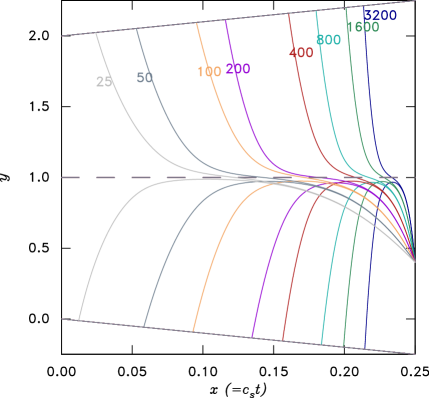
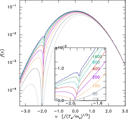
(a)                                                           (b)                                                          

Figure 5: (a) Marginal orbits for a range of mass ratio $m_{i}/m_{e}=m_{r}^{-1}=$ 25, 50, 100, 200, 400, 800, 1600, 3200. (b) Electron distribution functions at the final point (0.25,0.4), for these parameters. The insert expands the display of the unstable region of velocity space, plotting $f(v)$ on a linear scale.

In Fig. 5 are shown marginal orbit examples for a range of $m_{r}^{-1}$ values. The reduction of mass ratio leads to increasing drift effect. Tracking back the marginal orbits, their starts are increasingly closer to the object. The resulting distribution functions are plotted in Fig. 5(b). Lower mass-ratio cases show wider and deeper distribution minima. Formally, all the distributions of Fig. 5 are Penrose unstable. The linear inset close-up of the marginal velocity region clearly shows a minimum in $f(v)$. Although it arises from effects that cause a difference between reflected and unreflected orbits its occurrence requires no asymmetry in the distant distribution. The bump-on-tail of the case corresponding to nature ($m_{i}/m_{e}\sim 1600$) is fairly small and the minimum narrow, compared with the enhanced-electron-mass cases.

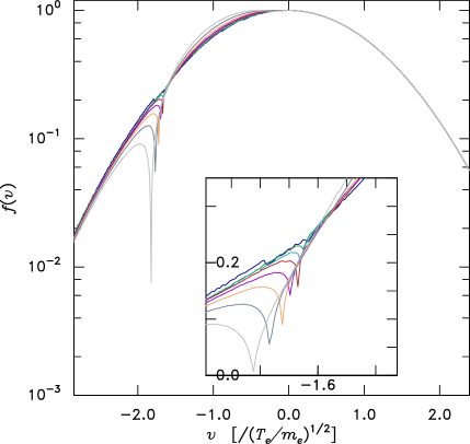
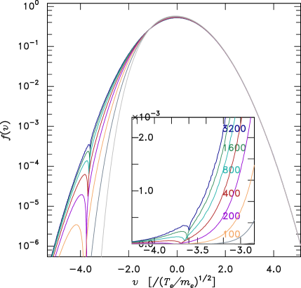
(a)                                                           (b)                                                          

Figure 6: Velocity distributions for a range of mass ratio $m_{i}/m_{e}=m_{r}^{-1}=$ 25, 50, 100, 200, 400, 800, 1600, 3200 . (a) Final point (1.0,-1.05). (b) Final point (0.15,-0.05).

If we choose a point out on the edge of the wake region or even outside it, such as is shown in Fig. 6(a) for position (1.0,-1.05), then there is no suppression of the peak of the distribution. It is equal to unity, the normalized value in the external plasma. At this position, while a deep hole is present in $f(v)$ for large electron mass, the distribution at physical mass ratio is practically stable within the noise level of the calculation.

In contrast, when the point of interest moves closer to the object (smaller $x$) as in Fig. 6(b), the marginal velocity is further out on the tail of distribution function. An unstable minimum is present; but it is at a distribution height that is very small, $\sim 10^{-4}$ of the peak. As $x$ is decreased still further the instability strength is eventually actually reduced to a negligible level as the gaussian tail decay becomes predominant.

These velocity trends arise, of course, because the height of the potential hill at position $(x,1)$ is equal to $\ln(\cosh(1+1/x))$, which approximately determines the corresponding marginal ($f$-minimum) velocity $v\approx 2\sqrt{(T_{e}/m_{e})\ln(\cosh[(1-y)/x])}$.

5 Nonlinear perturbation magnitude

To quantify the instability’s significance for unstable electron distributions it is helpful to use a quasilinear estimate of the final state of the distribution function after the instability has grown and saturated. This is based upon the approximation illustrated in Fig. 7.

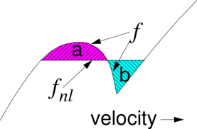
(a)                                                           (b)                                                          

Figure 7: (a) Quasi-linear evolution of the distribution function is assumed to be from the initial state, $f$, to a final distribution, $f_{nl}$, where the unstable region is flattened by mixing. That flat region is taken to connect continuously to the initial distribution at its ends, and to conserve particles. (Area a = Area b.) (b) A plot of the actual numerical flattening process for distributions with $m_{i}/m_{e}=m_{r}^{-1}=$ 25, 50, 100, 200, 400, 800, 1600, 3200, and final position (0.6,0). The flattened plateau is shown by the dashed line. Individual velocity points are shown for the uppermost case (3200) to indicate resolution.

The distribution is presumed to flatten in its unstable region by quasilinear diffusion, conserving particles. It is taken to connect continuously to the unperturbed distribution at the edge of the region of flattening. This specification uniquely defines the final state, whose energy is lower than the initial state. The energy loss from the resonant particles ($\Delta{\cal E}$) can readily be evaluated by integration. It generally goes equally into wave energy and heating of the bulk electron distribution[23]. So it represents approximately twice the saturated turbulent wave energy expected to be induced by the instability. The ratio of the resonant particle energy loss to the total thermal energy (${\cal E}_{0}$) of the pre-flattening electron distribution, gives a useful quantitative measure of the strength of the instability. The rounding error of the present calculations becomes increasingly dominant below $\Delta{\cal E}/{\cal E}_{0}\ \hbox to0.0pt{\raise 2.58334pt\hbox{$<$}\hss}\lower 2.15277pt\hbox{$\sim$}\ 10^{-6}$, so distributions giving less than that cannot be accurately assessed here. The background Langmuir turbulence present in the solar wind is observed to be up to $\sim 10^{-6}$ of ${\cal E}_{0}$ [24], so where numerically significant resonant energy loss is found, it is well above levels in the unperturbed solar wind.

For each distribution function, of the type illustrated in Figs. 5, 6 (but for a single specific mass ratio, $m_{r}$) the values of $\Delta{\cal E}$ and ${\cal E}_{0}$ are calculated using direct numerical integration. We perform a large number of such calculations over a 20 by 20 grid of positions throughout the $x$$y$-plane and display the results as a contour plot of $\log_{10}(\Delta{\cal E}/{\cal E}_{0})$ in Fig. 8.

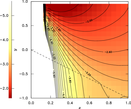
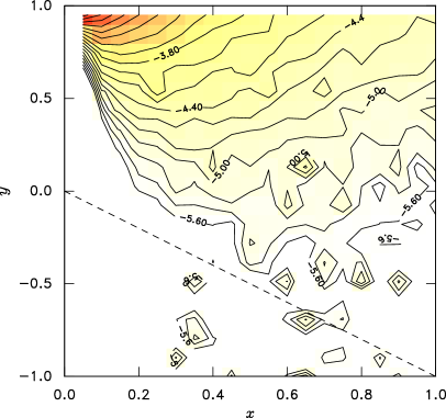
(a)                                                           (b)                                                          

Figure 8: Contours (spaced by 0.2) of the relative instability strength $\log_{10}(\Delta{\cal E}/{\cal E}_{0})$ over the wake $xy$-plane. (a) $m_{i}/m_{e}=25$, (b) $m_{i}/m_{e}=1835$. Geometry as in Fig. 1. The $y$-units are object-radii, and the perpendicular distance in object-radii is equal to the perpendicular Mach number ($v_{\perp}/c_{s}$) times $x$.

We observe that with artificially enhanced electron mass, so that $m_{i}/m_{e}=25$, most of the wake region is unstable (Fig. 8(a)). Indeed, that instability extends into the external region where potential is undisturbed (i.e. to $y<-x$). The only positions that are not unstable are at very small $x$. There the distribution function is completely depleted at the marginal velocity, in the way illustrated by Fig. 6(b). The strongest instability occurs near the wake symmetry axis ($y=1$) where a substantial bump-on-tail occurs like that illustrated in Fig. 5. The total electron density (and energy density) itself is also substantially depleted there, which contributes to the enhancement of the relative resonant energy loss by lowering ${\cal E}_{0}$.

In contrast, for realistic mass ratio $m_{i}/m_{e}=1835$ (Fig. 8(b)) the instability strength is greatly reduced: by roughly two orders of magnitude. (Fig. 8 is of the logarithm of instability strength.) The qualitative spatial distribution of instability strength is fairly similar to Fig. 8(a) but because it is quantitatively so much smaller, it reaches approximately the noise level at the edge of the wake’s perturbed potential region. Roughly speaking, the instability is significant for $y>0$, i.e. throughout the geometric wake.

Intermediate mass ratios give contour plots intermediate between the two shown. The trend is illustrated in Fig. 9 for the instability strengths at several fixed points.

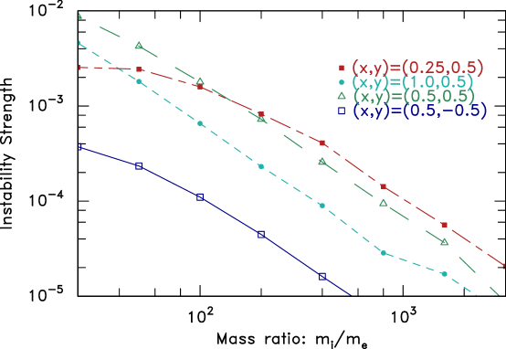
Figure 9: Variation of instability strength, $\Delta{\cal E}/{\cal E}_{0}$, with mass ratio for several end-points.

The curves of $\Delta{\cal E}/{\cal E}_{0}$ versus $m_{i}/m_{e}$ fall almost linearly in this logarithmic plot as $m_{i}/m_{e}$ increases, with slope slightly steeper than -1. There is no reduced threshold at which a mass ratio is sufficiently large to give quantitative results comparable to nature. One simply has to use the correct mass ratio.

The analytic potential approximations of “linear $\phi$” and “flat-top $\phi$” have also been explored to determine their instability strength. It is found that the linear $\phi$ gives substantially weaker instability, and the flat-top gives substantially stronger instability (by factors between 10 and 100). This observation demonstrates that the spatial profile shape of the potential plays a major role in determining the strength of the instability. Flat-top is more unstable because the marginal orbits spend more time near the potential peak. Linear is less unstable because they spend less. This effect is sufficiently strong that the uncertainties in the potential profile shape arising from the various approximations of the ion problem solution may significantly affect the numerical values of the instability strength. Therefore while the contour plots shown give a correct order of magnitude instability strength, they cannot be considered precise.

One should note that, because it is expressed in scaled units, Fig. 8 is essentially a universal figure. The value of the instability strength is not dependent upon plasma parameters such as density or temperature so long as the Debye length and Larmor radius are small compared with the object. Nor does it depend on object size or drift Mach number. It does require the external electron distribution to be well represented by a Maxwellian. Naturally non-thermal external electron velocity distributions such as might be represented by kappa-distributions, will affect the instability strength. However, the mechanism by which instability arises is the same no matter what the external distribution is; and, notably, it does not require non-thermal electron distributions.

For comparison, the values of the fractional quasi-linear energy loss $\Delta{\cal E}/{\cal E}_{0}$ for the unstable distributions arising in the energy-conserving case with external distribution shift, Fig. 3, are (a) $8.5\times 10^{-4}$, and (b) $1.8\times 10^{-3}$. Thus, inside the wake, the instability arising from energy non-conservation is of the same order of magnitude as would arise from a major external electron velocity shift: 0.2 times thermal. The level of electric field fluctuation energy in thermal equilibrium is ${\cal E}_{0}$ multiplied by a factor $\sim 1/(n_{e}\lambda_{De}^{3})$. That factor, for the solar wind, is of order $10^{-10}$. So all the turbulent energy levels discussed here are many orders of magnitude higher than thermal.

6 Oblique magnetic-field/drift

When the magnetic field and the drift velocity (of the plasma past the object) are not perpendicular, the solutions we have presented still apply immediately when interpreted in a way that this section describes. We continue to use coordinates in which the magnetic field is in the $y$-direction. The drift velocity is now oblique in the $xy$-plane. (This is a different choice of coordinates from what is generally adopted in the space-physics community when discussing wakes; they take the $x$-axis along the drift velocity). In these magnetic-field coordinates, an oblique external drift is completely equivalent to prescribing that in addition to the fixed perpendicular drift velocity $v_{\perp}$ (in the $x$-direction), the ions in the external region have a non-zero parallel velocity relative to the object $v_{\parallel\infty}$ [25, 12]. Since the quasi-neutral equations are entirely hyperbolic, as we have noted earlier, the $x$-coordinate is equivalent to the time, $t$. In effect, the abscissa of our plots can be considered either the distance from the object in its frame of reference, or the time since passing the object in the frame of the perpendicularly drifting plasma. In a frame of reference moving at speed $v_{\parallel\infty}$ in the $y$-direction with respect to the object, the external parallel ($y$) velocity is zero. The solution of the wake problem in this plasma-frame is of precisely the form we have considered above, except that the object is moving with $y$-speed $-v_{\parallel\infty}$. Because we are approximating the object as foreshortened in the scaled coordinates so that its edge radius of curvature is negligible, the fact that it is moving is irrelevant to the solution. When the $x$-axis is interpreted as the time $c_{s}t$ since the particular vertical slice of plasma passed the object, the graphs we have plotted previously apply without alteration. If, instead, one were to plot a snap-shot of the 2-dimensional spatial variation at a particular instant of time, however, the $xy$ plane would be sheared by the $-v_{\parallel\infty}$ motion. This shearing is purely geometrical. It amounts to the replacement of the $y$ spatial coordinate with $y^{\prime}=y-v_{\parallel\infty}t=y-(v_{\parallel\infty}/c_{s})x$. Although this shearing may be large (because of high Mach number) in the coordinates we have been using, it does not affect the equations for the ion or electron dynamics.

Therefore, the solutions we have obtained above apply directly to cases with finite external parallel ion drift, provided that they are interpreted as being the solutions as a function of time, in the plasma frame of reference.

The question then arises as to what the external electron velocity distribution actually is, in this plasma reference frame. Is it symmetric or not? Since $v_{\parallel\infty}$ is typically $\sim 10c_{s}$ for the moon in the solar wind, the frame’s velocity is a significant fraction, $\sim 0.2$, of the electron thermal velocity. If, then, the electron parallel distribution were a stationary Maxwellian in the rest frame of the moon, it would be substantially shifted in the moving frame and the effects of section 3 would immediately apply. However, it can be shown from considerations of magnetic field gradient that the total electric current density in the solar wind must be far less than would be implied by a relative velocity of electrons and ions of $0.2v_{e}$. Therefore, in fact the mean electron and ion speeds are very nearly equal in the external wind. That means the electron distribution is unshifted in the parallel-moving reference frame, and the effects discussed in section 3 do not arise from parallel drift (though they might arise from higher-order electron distribution asymmetry such as skewness).

7 Summary

Two mechanisms by which unstable parallel electron velocity distributions can arise in a magnetized plasma wake have been explored. First (section 3) substantial asymmetry of the external velocity distribution, for example an overall parallel drift, can be turned into instability by the wake’s potential structure. However, limits on electric current density in the solar wind near the moon (for example) prevent average electron drift alone from being large enough to generate major instability. Second (section 4) the non-conservation of electron parallel energy in the perpendicular drift also gives rise to unstable distribution minima near the marginal electron velocity that only just traverses the potential energy hill of the wake. The electron distributions have been calculated for collisionless orbits, and the turbulence energy density to which they would give rise has been evaluated quasi-linearly. The instability is found to be everywhere in the wake quite significant, and fairly strong near the wake axis. If artificially large electron mass is used, as is frequently the case in simulations that treat both electrons and ions by PIC techniques, then this instability effect is greatly enhanced; so their results will not be in quantitative agreement with nature.

Hybrid PIC simulations which proceed to the opposite extreme — infinitesimal electron mass (e.g. [7, 8, 2])— obviously omit the parallel electron instability completely; but since they make no pretence of treating the details of the electron dynamics, they will perhaps be less likely to be misleading. There are of course many other ion and anisotropy instability mechanisms that will perturb the electrons. The present work establishes the approximate Langmuir turbulence level arising from the electron parallel distribution, with which these other mechanisms will compete.

References

-
[1]
J. S. Halekas, V. Angelopoulos, D. G. Sibeck, K. K. Khurana, C. T. Russell, G. T. Delory, W. M. Farrell, J. P. McFadden, J. W. Bonnell, D. Larson, R. E. Ergun, F. Plaschke, and K. H. Glassmeier, Space Science Reviews(Jan. 2011), doi:“bibinfo–doi˝–10.1007/s11214-010-9738-8˝,
http://www.springerlink.com/index/10.1007/s11214-010-9738-8 -
[2]
S. Wiehle, F. Plaschke, U. Motschmann, K.-H. Glassmeier, H. Auster, V. Angelopoulos, J. Mueller, H. Kriegel, E. Georgescu, J. Halekas, D. Sibeck, and J. McFadden, Planetary and Space
Science 59, 661 (Jun. 2011),
http://linkinghub.elsevier.com/retrieve/pii/S0032063311000407 -
[3]
L. Patacchini and I. H. Hutchinson, Plasma Physics and
Controlled Fusion 52, 035005 (Mar. 2010),
http://stacks.iop.org/0741-3335/52/i=3/a=035005 -
[4]
I. H. Hutchinson and L. Patacchini, Plasma Physics and
Controlled Fusion 52, 124005 (Dec. 2010),
http://stacks.iop.org/0741-3335/52/i=12/a=124005 -
[5]
K. W. Ogilvie, J. T. Steinberg, R. J. Fitzenreiter, C. J. Owen, A. J. Lazarus, W. M. Farrell, and R. B. Torbert, Geophysical Research Letters 23, 1255 (1996),
http://www.agu.org/journals/ABS/1996/96GL01069.shtml -
[6]
J. S. Halekas, S. D. Bale, D. L. Mitchell, and R. P. Lin, Journal of Geophysical
Research 110, A07222 (2005),
http://www.agu.org/pubs/crossref/2005/2004JA010991.shtml -
[7]
E. Kallio, Geophysical Research
Letters 32, 1 (2005),
http://www.agu.org/pubs/crossref/2005/2004GL021989.shtml -
[8]
P. Trávníček, Geophysical Research
Letters 32, 4 (2005),
http://www.agu.org/pubs/crossref/2005/2004GL022243.shtml - [9] A. V. Gurevich, L. P. Pitaevskii, and V. V. Smirnova, Space Science Reviews 9, 805 (1969)
-
[10]
A. V. Gurevich and L. P. Pitaevsky, Progress in Aerospace
Sciences 16, 227 (1975),
http://linkinghub.elsevier.com/retrieve/pii/0376042175900160 -
[11]
U. Samir, K. H. Wright, and N. H. Stone, Reviews of Geophysics 21, 1631 (1983),
http://www.agu.org/pubs/crossref/1983/RG021i007p01631.shtml -
[12]
I. H. Hutchinson, Physics of Plasmas 15, 123503 (2008),
http://link.aip.org/link/PHPAEN/v15/i12/p123503/s1&Agg=doi -
[13]
L. Patacchini and I. Hutchinson, Physical Review E 80, 1 (Sep. 2009),
http://link.aps.org/doi/10.1103/PhysRevE.80.036403 -
[14]
C. Sack and H. Schamel, Physics Reports 156, 311 (Dec. 1987),
http://linkinghub.elsevier.com/retrieve/pii/0370157387900391 - [15] G. Manfredi, S. Mola, M. R. Feix, A. De, R. Scientifque, and O. Cedex, Physics of Fluids B 5, 388 (1993)
-
[16]
M. A. Hellberg, T. K. Baluku, I. Kourakis, and N. S. Saini, Physics of Plasmas 16, 094701 (2009),
http://link.aip.org/link/PHPAEN/v16/i9/p094701/s1&Agg=doi - [17] N. Meyer-Vernet, M. Moncuquet, and S. Hoang, Icarus 116, 202 (1995)
- [18] W. M. Farrell, M. L. Kaiser, J. T. Steinberg, and S. D. Bale, Journal of Geophysical Research 103, 23,653 (1998)
-
[19]
P. C. Birch and S. C. Chapman, Physics of Plasmas 8, 4551 (2001),
http://link.aip.org/link/PHPAEN/v8/i10/p4551/s1&Agg=doi -
[20]
W. M. Farrell, T. J. Stubbs, J. S. Halekas, G. T. Delory, M. R. Collier, R. R. Vondrak, and R. P. Lin, Geophysical Research
Letters 35, 1 (Mar. 2008),
http://www.agu.org/pubs/crossref/2008/2007GL032653.shtml - [21] P. J. Kellogg, K. Goetz, S. J. Monson, J. Bougeret, R. Manning, and M. L. Kaiser, Geophysical Research Letters 23, 1267 (1996)
- [22] G. Schmidt, Physics of High Temperature Plasmas, 2nd ed. (Academic Press, New York, 1979)
- [23] R. C. Davidson, Methods in Nonlinear Plasma Theory (Academic Press, New York, 1972)
- [24] Y. L. Alpert, The near-Earth and interplanetary plasma, Volume 2 (Cambridge University Press, Cambridge, 1983) p. 221
-
[25]
I. H. Hutchinson, Physical Review
Letters 101, 035004 (Jul. 2008),
http://link.aps.org/doi/10.1103/PhysRevLett.101.035004